Cross-Site Cross-Season PV Power via Lightweight ELM with Two Residual Layers and Calibration

Abstract

Accurate photovoltaic (PV) power forecasting degrades when models are deployed across sites or seasons, primarily due to distribution shift (amplitude bias and scale mismatch) and anomalous contamination—with pronounced amplitude–phase errors during rapidly changing cloud passages. To address this, we propose Res2-ELM-C, a lightweight Extreme Learning Machine framework featuring three-stage residual stacking—main fit, first-order residual, and near-orthogonal residual—fused via a non-negative ridge-gated mechanism learned on a time-delayed validation window. Robust scaling and a two-step linear calibration—constant de-biasing followed by per-hour gain alignment—mitigate out-of-distribution drift and enhance peak tracking under rapidly varying conditions. In a unified evaluation protocol, the proposed approach consistently reduces MAE/RMSE/MAPE relative to standard baselines while maintaining ELM-level training and inference complexity. These properties make Res2-ELM-C suitable for quasi-real-time day-ahead/intraday dispatch and distributed energy management system applications.

1. Introduction

As PV capacity and grid penetration rise, forecasting has become a core module in operations and DER-EMS. Forecast errors propagate into day-ahead/intraday bidding, reserves and storage scheduling, and ultimately operating costs; recent studies quantify the economic value of integrating probabilistic solar forecasts into market participation and scheduling [1,2]. Public benchmarking and recent reviews have also standardized probabilistic evaluation and data protocols, shaping engineering practice [3]. In system operations, scenario/probabilistic forecasts are increasingly used for reserve allocation and risk-constrained optimization [1,4].

Unlike conventional “fixed-site deployment”, real-world practice often requires cross-site, cross-season, and cross-weather transfer and reuse—for example, training on January and April histories while inferring for September (seasonal look-ahead). Systematic seasonal and spatial changes in solar elevation, cloud regimes, and surface albedo induce pronounced distribution shifts in the input–output mapping, typically manifesting as amplitude bias and scale mismatch and, during rapid cloud passages, as coupled amplitude–phase errors (peak magnitude and timing failing to align). To explicitly quantify out-of-domain degradation, we define the generalization ratio (GenRatio) as ${\displaystyle \frac{{\mathbf{R}\mathbf{M}\mathbf{S}\mathbf{E}}_{\mathbf{O}\mathbf{O}\mathbf{D}}}{{\mathbf{R}\mathbf{M}\mathbf{S}\mathbf{E}}_{\mathbf{I}\mathbf{D}}}}$; values closer to one indicate better cross-domain robustness. We report GenRatio alongside MAE, MAPE, and Pearson’s $\mathit{r}$. In operation, missingness and contamination can further compound these shifts, exacerbating the difficulty of peak tracking and phase alignment.

Method families offer complementary strengths. Mechanistic/NWP-driven chains provide physical consistency yet incur external data dependence and latency; recent satellite-based and hybrid DL–physics works make these trade-offs explicit [5,6]. Visual/remote-sensing inputs (geostationary satellites, all-sky imagers) are pivotal from minutes to hourly horizons; new CNN/Transformer pipelines and hybrid model-chains have advanced short-term cloud-shadow tracking and cross-site robustness [7,8,9]. On the data-driven side, compact Transformer/TCN baselines have matched or exceeded classical ML while remaining deployable [10]. For calibration and uncertainty, modern post-processing (EMOS/quantile regression; optimal combination of calibrated quantiles) improves probabilistic reliability for trading and operations [11]. For lightweight edge deployment, ELM variants remain competitive due to minimal training/inference overhead; recent optimized ELM forecasters further confirm this trend [12].

Robust spatiotemporal frameworks enhance performance outside the calibration domain, but significantly increase structural complexity and data dependency [13]. At minute-to-hourly temporal scales, visual/remote-sensing information becomes crucial for tracking rapid power transitions caused by cloud shadows: spatiotemporal textures from all-sky cameras and geostationary meteorological satellites can be coupled with learning models for predictive modeling of short-term cloud evolution [14,15,16,17]. On the other hand, probabilistic and post-processing approaches (e.g., model-chain calibration, EMOS/quantile regression) emphasize calibration and uncertainty representation. However, loose coupling with the main model may introduce statistical inconsistencies and maintenance complexity [18,19]. For engineering-ready lightweight approaches, Extreme Learning Machines (ELMs) are widely adopted in edge computing and resource-constrained deployments due to their minimal training/inference overhead, giving rise to various improved variants [20].

In practice there is a multi-objective trade-off among complexity, latency, and robustness: heavy external pipelines may raise latency and maintenance costs; loosely coupled post-processing risks statistical inconsistency; and a single learner under strong drift struggles to absorb both bias and scale mismatch. This motivates a lightweight, interpretable, calibratable, and transferable all-in-one framework.

Against this backdrop, we propose Res2-ELM-C, a lightweight framework for cross-site/season deployment. The goal is to enhance OOD robustness and peak/phase alignment without increasing inference complexity or latency, by combining structured error modeling with linear, auditable calibration. Building on an ELM-level nonlinear base learner, we explicitly decompose errors into three progressive residual stages (main trend, first-order residual, and an orthogonal residual), and fuse them using non-negative ridge gating on a delayed validation window (weights α, β ≥ 0) for interpretability. A two-step linear calibration (constant de-biasing and linear rescaling) then corrects bias/gain under a unified statistical protocol, enabling hour-level maintenance and practical operations.

Research on photovoltaic power forecasting spans mechanistic/NWP, data-driven, visual/remote-sensing, transfer, and probabilistic post-processing tracks. Recent satellite/ASI studies and benchmarks have provided a de facto coordinate system for standardized comparisons across methods, data protocols, and horizons [14,15,16,17]. Within mechanistic/NWP chains, the physical “meteorology–irradiance–power” linkage ensures cross-scale consistency and interpretability, but the end-to-end pipeline is long and depends strongly on external data and compute [17,19].

The data-driven paradigm has progressed from sparse/linear models to compact deep learners (e.g., Transformer/TCN), yet robustness under seasonal/site drift—manifesting as bias and scale mismatch—remains challenging [21]. Pattern-based segmentation (e.g., weather-type clustering or SOM) mitigates heterogeneity but cannot fully absorb spatiotemporal coupling and pollution anomalies [22,23]. Robust spatiotemporal frameworks can improve accuracy outside the calibration domain, yet often increase structural complexity and data dependency [13].

At minute-to-hourly horizons, visual/remote-sensing inputs are pivotal: spatiotemporal textures from all-sky imagers and geostationary satellites, when integrated with CNN/RNN/Transformer encoders or hybrid DL–physics chains, enable short-term cloud evolution nowcasting and enhance cross-site robustness [14,15,16,17]. For cross-station/season transferability under data scarcity and out-of-domain shift, recent transfer-learning and multimodal ViT pipelines demonstrate additional value, complementing satellite/ASI fusion strategies [15,16,24].

In parallel, probabilistic/post-processing methods—such as EMOS/quantile regression and model-chain calibration—improve calibration and uncertainty representation, though loose coupling with the main learner can introduce statistical inconsistency and maintenance burden [18,19]. For lightweight edge deployment, ELM variants remain attractive due to minimal training/inference overhead and online adaptability [20]. Synthesizing these trends reveals a complexity–latency–robustness trade-off: heavy external pipelines raise latency and maintenance costs; loosely coupled post-processing risks inconsistency; and single learners under strong drift struggle to absorb both bias and gain mismatch. Therefore, there is a need for a lightweight, interpretable, calibratable, and transferable framework under a unified, leakage-free evaluation protocol that improves out-of-domain performance within real-time constraints while reducing maintenance complexity [19,20,21].

A comparative summary of representative forecasting methods, highlighting their inputs–outputs, data scale, metrics, robustness, and complexity–parameter efficiency–physics adaptivity, is provided in Table 1. This overview underscores the trade-offs in current approaches, such as the high complexity of deep learning models versus the lightweight efficiency of ELM variants.

Table 1. Comparative summary of representative forecasting methods: inputs–outputs, data scale, metrics, robustness, and complexity–parameter efficiency–physics adaptivity.

Representative Work	Input → Output	Data Scale	Advantages/Limitations (Key Points)	Indicators/Benefits (Examples)	Structural Complexity (0–10)	Parameter Efficiency (0–10 ↑)	Physical Mechanism Adaptivity (0–5)
Mechanistic/NWP chain —Wang et al., RSER 2024 [2]	Hourly updated NWP → day-ahead/intraday GHI/PV	System-level; rolling day-ahead/intraday	Adv. Physically consistent; market-aligned horizons. Lim. External feeds; higher latency/compute.	Economic value quantified; NRMSE/CRPS ↓ vs. persistence/empirical baselines.	8.3 (High)	5.5 (Medium)	5 (High)
Satellite DL “model-chain” —Chen et al., ECM 2024 [8]	GEO satellite (≈2 km/5 min) → 15–180 min GHI (two-stage DL)	Multi-site; multi-horizon	Adv. Better spatial GHI then multi-step forecasting; stronger ramp detection. Lim. Maintenance and external dependence.	nRMSE ↓, skill ↑ vs. end-to-end or physics–DL hybrids.	8.0 (High)	5.0 (Medium)	4 (High)
All-sky/Multimodal Transformer—Liu et al., Appl. Energy 2023 [16]	All-sky images + meteorology → ultra-short-term GHI	Single/multi-site; ≈10 min ahead	Adv. Vision–temporal fusion; high short-window accuracy. Lim. Camera upkeep/calibration.	NRMSE ≈ 4.28% (10 min); outperforms multiple SOTA baselines.	5.3 (Medium)	6.0 (Medium–High)	3 (Medium)
Compact Transformer for PV—Piantadosi et al., Energy & AI 2024 [10]	Hist. power + weather (opt. visual feats) → 15–60 min PV	Multi-site; seasonal splits	Adv. Compact; fast inference. Lim. Under strong drift, bias/scale mismatch persists.	NMAE/NRMSE ≤ classical ML; stable CPU latency.	3.7 (Medium–Low)	7.0 (High)	2 (Medium–Low)
This work—Res2-ELM-C (lightweight residual + hour-wise calibration)	Historical PV + exogenous features → hour-ahead PV	Six sites; hourly; chronological split (DC/AC ≈ 1.2–1.3; 24-parameter hourly calibration for OOD.	Adv. Two residual layers with non-negative ridge gating; Lim. Conventional multi-step setup;	OOD RMSE ↓ 19.4–31.6% vs. classical baselines; ≈0.9995; MAPE ≈ 2.25%; per-point inference ≈ 23.9 μs on CPU.	2.5 (Low)	8.0 (High ↑)	3.5 (Medium–High)

Labels: High/Medium/Low follow the rubric in the manuscript; ↑ indicates higher is better. ↓ indicates lower is better. Abbreviations: GEO—geostationary satellite; DL—deep learning; NWP—numerical weather prediction; SOTA—state of the art. Structural complexity/parameter efficiency/physical mechanism adaptivity use relative scales (0–10, 0–10 ↑, and 0–5, respectively). Lower complexity = simpler pipeline and fewer external dependencies; higher parameter efficiency = fewer parameters for a given accuracy; higher physics adaptiveness = stronger explicit calibrability and compatibility with the $\mathbf{m}\mathbf{e}\mathbf{t}\mathbf{e}\mathbf{o}\mathbf{r}\mathbf{o}\mathbf{l}\mathbf{o}\mathbf{g}\mathbf{y}\to \mathbf{i}\mathbf{r}\mathbf{r}\mathbf{a}\mathbf{d}\mathbf{i}\mathbf{a}\mathbf{n}\mathbf{c}\mathbf{e}\to \mathbf{p}\mathbf{o}\mathbf{w}\mathbf{e}\mathbf{r}$ chain. Parameter counts are an order-of-magnitude under typical small configurations; values may vary with hyperparameters. All indicators reflect leakage-free chronological splits with daytime mask. $\mathbf{G}\mathbf{e}\mathbf{n}\mathbf{R}\mathbf{a}\mathbf{t}\mathbf{i}\mathbf{o}={\mathbf{R}\mathbf{M}\mathbf{S}\mathbf{E}}_{\mathbf{O}\mathbf{O}\mathbf{D}}/{\mathbf{R}\mathbf{M}\mathbf{S}\mathbf{E}}_{\mathbf{I}\mathbf{D}}$ and CRPS/PIT applies to probabilistic methods. For “This work”, CPU inference ≈ 23.9 μs/point and OOD RMSE reductions (19.4–31.6%) are measured under the reported three-site hour-ahead protocol (Train M01/M04 → Test M07; fixed vs. single-axis; 5–50 MW; DC/AC ≈ 1.20–1.30).

To accommodate cross-site/cross-season deployment scenarios and enhance accuracy under significant distribution drift, the main contributions of this work are summarized as follows:

• To address cross-domain accuracy degradation, we propose a lightweight three-stage residual (main + two residual layers) decomposition framework. To address accuracy degradation caused by amplitude bias, scale mismatch, and peak amplitude–phase misalignment, we construct a three-stage residual (main + two residual layers) structure: “main fit–first-order residual–orthogonal residual”. Within the residual channel, we introduce quantile-driven robust range mapping and NNLS pre-scaling orthogonalization to reduce inter-layer collinearity and enhance peak fitting capability for rapidly changing cloud shadows.
• We propose an interpretable fusion mechanism combining non-negative ridge regression gating with two-step linear calibration. Within the time-delayed validation window, non-negative ridge regression performs weight learning on layer outputs to avoid negative gains and suppress overfitting. Subsequently, a two-step linear calibration (“constant bias removal + hourly gain alignment”) eliminates systematic bias and dimensional differences under a unified statistical metric, thereby stably improving OOD accuracy without altering the main model structure.
• We achieve robust accuracy gains under unified evaluation protocols while maintaining ELM-level complexity. Comparisons use unified metrics including time-sequence partitioning(training/test ≈ 80:20, tail validation window), daytime criteria (solar elevation angle > 5°), and floor-based MAPE. Across multiple sites and seasons, it consistently reduces MAE/RMSE/MAPE across multiple sites and seasons, with a significant peak RMSE reduction. Training and inference complexity remain comparable to ELM, achieving single-threaded inference latency at the microsecond level, making it suitable for edge computing and near-real-time applications.

2. Materials and Methods

2.1. PV Characteristics and Forecasting Background

Photovoltaic (PV) power output is jointly determined by physical factors, including irradiance, angle of incidence, and module temperature: the plane-of-array irradiance (plane-of-array, ${\mathbf{G}}_{\mathbf{P}\mathbf{O}\mathbf{A}}$) is influenced by the superposition of direct normal irradiance (DNI), diffuse horizontal irradiance (DHI), and surface albedo; solar altitude and azimuth determine the geometric incidence angle; and module temperature ${\mathbf{T}}_{\mathbf{c}\mathbf{e}\mathbf{l}\mathbf{l}}$ increases with ambient temperature and irradiance loading, thereby altering efficiency and introducing thermally induced deviation (temperature coefficient). DC-side power can be approximated as

$${\mathbf{P}}_{\mathbf{D}\mathbf{C}}\approx {\mathsf{\eta }}_{\mathbf{m}\mathbf{o}\mathbf{d}}\left({\mathbf{G}}_{\mathbf{P}\mathbf{O}\mathbf{A}},{\mathbf{T}}_{\mathbf{c}\mathbf{e}\mathbf{l}\mathbf{l}}\right)\cdot {\mathbf{G}}_{\mathbf{P}\mathbf{O}\mathbf{A}}\cdot \mathbf{A}$$

(1)

$${\mathit{T}}_{\mathbf{c}\mathbf{e}\mathbf{l}\mathbf{l}}\approx {\mathit{T}}_{\mathbf{a}\mathbf{m}\mathbf{b}}+\mathit{\kappa }\cdot {\mathit{G}}_{\mathbf{P}\mathbf{O}\mathbf{A}}$$

(2)

The AC side is constrained by inverter efficiency and rated power: ${\mathit{P}}_{\mathbf{A}\mathit{C}}\left(\mathbf{t}\right)=\mathbf{min}\left\{\mathsf{\eta }\mathbf{i}\mathbf{n}\mathbf{v}\left({\mathit{P}}_{\mathbf{D}\mathbf{C}}\left(\mathbf{t}\right)\right)\cdot {\mathit{P}}_{\mathbf{D}\mathbf{C}}\left(\mathbf{t}\right),{\mathit{P}}_{\mathbf{r}\mathit{a}\mathit{t}\mathit{e}\mathit{d}}\right\}.$ Shearing/clipping is prone to occur under high irradiance conditions; grid constraints such as curtailment/AGC/AVC further alter the AC-side profile. Additionally, shading, soiling, and fast-moving cloud edges induce amplitude–phase coupling errors (simultaneous shifts in peak height and arrival time). Seasonal and site variations in solar geometry, cloud types, and surface albedo cause distribution drift (amplitude bias and scale mismatch), constituting the primary source of accuracy degradation in cross-site/cross-season deployments.

To facilitate understanding of the energy chain and disturbance locations, Figure 1 provides an overview from meteorological drivers → incident geometry and ${\mathbf{G}}_{\mathbf{P}\mathbf{O}\mathbf{A}}$ → module/array ${\mathit{P}}_{\mathbf{D}\mathbf{C}}$ → inverter and grid constraints → output ${\mathit{P}}_{\mathbf{A}\mathit{C}}$, highlighting the effects of fast cloud edges, shading/soiling, clipping, and control commands on curve morphology.

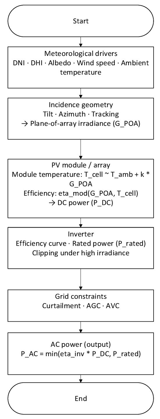
Figure 1. Overview of PV energy conversion and disturbance sources. From meteorological drivers (DNI/DHI, albedo, wind, ambient temperature) to incidence geometry and plane-of-array irradiance (${\mathit{G}}_{\mathit{P}\mathit{O}\mathit{A}}$), then module/array DC power (${\mathit{P}}_{\mathit{D}\mathit{C}}$, including temperature effects, shading, and soiling), followed by inverter and grid constraints yielding AC power (${\mathit{P}}_{\mathit{A}\mathit{C}}$). Callouts indicate fast cloud edges, clipping, and control actions (AGC/AVC). Note: * denotes multiplication.

${\mathbf{G}}_{\mathbf{P}\mathbf{O}\mathbf{A}}$ can be decomposed into three components: direct, diffuse sky, and surface reflection: ${\mathit{G}}_{\mathit{P}\mathit{O}\mathit{A}}={\mathit{B}}_{\mathit{P}\mathit{O}\mathit{A}}+{\mathit{D}}_{\mathit{P}\mathit{O}\mathit{A}}+{\mathit{R}}_{\mathit{g}}$, where ${\mathit{B}}_{\mathit{P}\mathit{O}\mathit{A}}=\mathit{D}\mathit{N}\mathit{I}·\mathbf{c}\mathbf{o}\mathbf{s}\mathit{\theta }\mathit{i}$ ($\mathit{\theta }\mathit{i}$ being the incident angle); ${\mathit{D}}_{\mathit{P}\mathit{O}\mathit{A}}$ is derived from scattering inversion models (e.g., ${\displaystyle \frac{\mathit{P}\mathit{e}\mathit{r}\mathit{e}\mathit{z}}{\mathit{H}\mathit{a}\mathit{y}}}-\mathit{D}\mathit{a}\mathit{v}\mathit{i}\mathit{e}\mathit{s}$); and $\mathit{R}\mathit{g}\propto \mathit{\rho }\mathit{g}$·GHI, which depends on array tilt angle. This decomposition explains the systematic seasonal and azimuth/tilt effects on ${\mathit{G}}_{\mathit{P}\mathit{O}\mathit{A}}$ and constitutes one physical source of subsequent “scale mismatch”. Module temperature can be approximated linearly as T $\mathit{c}\mathit{e}\mathit{l}\mathit{l}\approx \mathit{T}\mathit{a}\mathit{m}\mathit{b}+\mathit{\kappa }{\mathit{G}}_{\mathit{P}\mathit{O}\mathit{A}}$ (wind speed correction may also be introduced), with efficiency ${\mathit{\eta }}_{\mathit{m}\mathit{o}\mathit{d}}$ varying with Tcell and ${\mathit{G}}_{\mathit{P}\mathit{O}\mathit{A}}$; the inverter side typically employs segmented efficiency curves and is constrained by Prated. Shearing occurs under high irradiance, while scheduling or voltage/reactive power control introduces artificial curtailment, altering the ${\mathit{P}}_{\mathit{A}\mathit{C}}$’s peak and slope. $\mathit{P}\mathit{V}$ output exhibits multiscale variability: diurnal cycles control slow-changing profiles, seasonal scales alter the magnitude of effects, and minute-scale cloud shadows cause abrupt transitions. Typical forecasting horizon types include minute-level short-term (5–30 min), hour-level intraday (1–6 h), and day-ahead (24 h); different horizons involve distinct trade-offs between data sources and complexity. Figure 2 aligns time horizons with data sources (near-term measurements, all-sky/satellite, $\mathit{N}\mathit{W}\mathit{P}$, astronomical geometry) and correlates them with power operations (trading, dispatch, reserve) on the right.

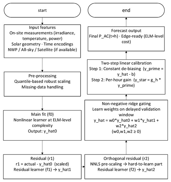
Figure 2. Time scales, forecast horizons, and information sources. Minute-scale nowcasting leverages proximal sensors and all-sky/satellite imagery; intra-hour to hourly horizons combine on-site measurements with short-range NWP; and day-ahead relies mainly on NWP and astronomical geometry. The right strip links horizons to grid-use cases (market bidding, dispatch, reserves).

As shown in Figure 2, this paper aligns photovoltaic power forecasting across “timescale–information source–power operations”: minute-scale short-term (5–30 min) primarily relies on near-site measurements and all-sky/satellite textures to characterize rapid cloud edge passage; the 1–6 h intraday time window requires combining site measurements with short-range NWP to balance timeliness and availability; and the 24 h period relies more heavily on NWP and astronomical geometry to ensure cross-day consistency. The operational bands on the right correspond to application stages such as market clearing, rolling dispatch, and reserve allocation. This approach directly constrains model design and deployment complexity: under stringent real-time and edge computing constraints, this paper prioritizes reusing lightweight information like proximity/geometry, while absorbing seasonal/site drift through an auditable “layered residual + linear calibration” path without increasing inference latency. In other words, Figure 2 explains the rationale for choosing a lightweight framework and employing calibration enhancement: the former addresses latency and maintainability, while the latter compensates for cross-domain dimensional and bias mismatches. This forms a consistent design loop with the physical link in Figure 1 and the calibration path in Figure 3.

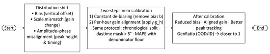
Figure 3. Distribution shift (bias and scale mismatch) and a unified two-step linear calibration path: constant de-biasing followed by per-hour gain alignment under the same evaluation protocol. The inset illustrates amplitude–phase misalignment in a fast-changing window and its mitigation after calibration.

To enhance comparability and robustness across sites/seasons, dimensionless normalization is often performed using power envelope clearance (${\mathit{P}}_{\mathit{c}\mathit{l}\mathit{e}\mathit{a}\mathit{r}}$) or nameplate capacity, defining the clearance index $\mathit{k}\mathit{\ast }={\displaystyle \frac{{\mathit{P}}_{\mathit{A}\mathit{C}}}{{\mathit{P}}_{\mathit{c}\mathit{l}\mathit{e}\mathit{a}\mathit{r}}}}$ to absorb dimensional differences. Input-side processing employs time alignment and time zone normalization, solar mask (solar elevation angle > 5°), outlier/missing data handling (e.g., winsorization and interpolation), and quantile-based robust scaling to mitigate pollution effects on training and evaluation. Cross-season/cross-site transfer introduces amplitude bias and scale mismatch, causing uncalibrated forecasts to exhibit systematic deviations in peak values and overall magnitude. Rapid cloud windows also induce amplitude–phase coupling, where peak height and arrival time shift simultaneously. Figure 3 illustrates a two-step linear calibration under unified evaluation metrics (time-sequence segmentation, daytime scope, MAPE denominator floor): first constant bias removal, then hourly gain alignment to correct scale and peak without altering main model complexity. At time t, we predict future active power ${\mathit{y}}_{\mathit{t}+\mathit{h}}$ at time $\mathit{t}+\mathit{h}$ using the historical window ${\mathit{X}}_{\mathit{t}-\mathit{L}:\mathit{t}}$ (field measurements, clear-sky index, solar geometry, NWP, time encoding, etc.).

$${\widehat{\mathit{y}}}_{\mathit{t}\mathbf{+}\mathit{h}}\mathbf{=}\mathit{f}\left({\mathbf{X}}_{\mathit{t}\mathbf{-}\mathit{L}\mathbf{:}\mathit{t}}\right)\mathbf{,}\mathit{h}\mathbf{\in }\left\{\mathbf{5}\mathbf{-}\mathbf{30}\mathbf{m}\mathbf{i}\mathbf{n}\mathbf{,}\mathbf{1}\mathbf{-}\mathbf{6}\mathbf{h}\mathbf{,}\mathbf{24}\mathbf{h}\right\}$$

(3)

Training and evaluation employ temporal segmentation and daytime windows, with metrics including MAE, RMSE, and MAPE with denominator floor. Cross-domain degradation is quantified using the GenRatio. Subsequent sections detail implementation specifics and complexity statistics for the base learner, three-stage residual (main + two residual layers) network, and non-negative ridge gate.

2.2. Forecasting Problem Formulation

This work formulates PV output forecasting as a multi-time-step point prediction problem: at time t, using a historical window ${\mathrm{X}}_{\mathrm{t}-\mathrm{L}:\mathrm{t}}$ of length L (containing on-site measurements, clear-sky index, solar geometry, NWP forecasts, and time encoding), we predict the active power $y_{t+h}$ at the future time t + h.

$$\begin{array}{c}{\widehat{y}}_{t+h}=f\left(X_{t-L:t}\right),h\in \mathcal{H}\end{array}$$

(4)

H covers temporal intervals of adjacent, intraday, and pre-day operations. Training and evaluation employ time-sequence segmentation and daytime criteria (solar elevation angle > 5°). Errors are calculated post-calibration, with metrics including MAE, RMSE, and MAPE with denominator floor. Cross-domain degradation is measured by the GenRatio. To mitigate the impact of anomalous pollution and extreme values, the input side employs quantile robust scaling and mild winsorization. On the output side, two-step linear calibration is performed under the same statistical metric to enhance consistency in peak values and overall scale. Subsequent sections detail the implementation of the base learner, three-stage residual (main + two residual layers) network, and non-negative ridge gate, followed by comparisons against several baselines under a unified metric.

We also report the Pearson correlation coefficient. All standardization, range mapping, and calibration parameters are estimated on the training segment and kept fixed during validation and testing.

Primary scalar metrics include the following:

2.3. Problem Definition and Notation

This paper investigates point forecasting of time-series photovoltaic (PV) power. Let the time-ordered sample be $\left\{\left({\mathit{x}}_{\mathit{t}}\mathbf{,}{\mathit{y}}_{\mathit{t}}\right)\right\}\mathit{N}$ where ${\mathit{x}}_{\mathit{t}}\mathbf{\in }{\mathbf{R}}^{\mathbf{d}}$ and includes the following: (i) Historical power block $\left[{\mathit{y}}_{\mathit{t}\mathbf{-}\mathit{L}\mathbf{:}\mathit{t}\mathbf{-}\mathbf{1}}\right]$; (ii) Numerical weather prediction (NWP) and/or surface meteorological data (e.g., GHI, air temperature T, wind speed WS, cloud cover, etc.); (iii) Time-based derived features (hour, day of the week, holidays, etc.). The target ${\mathit{y}}_{\mathit{t}}\mathbf{\in }\mathit{R}$ represents grid-connected active power. Unless otherwise specified, the resolution is 1 h with a prediction step size h = 1 (extendable to multiple steps).

Data is chronologically divided into training, validation, and test segments. The final 20% of the training segment serves as the validation window, used solely for estimating inter-layer weights and calibration parameters. The test segment is reserved exclusively for final evaluation to prevent information leakage. Evaluation is restricted to sunshine samples with solar elevation angle > 5°.

$$\mathbf{M}\mathbf{A}\mathbf{E}\mathbf{=}{\displaystyle \frac{\mathbf{1}}{\mathit{n}}}\sum _{\mathit{t}\mathbf{=}\mathbf{1}}^{\mathit{n}}\left|{\mathit{y}}_{\mathit{t}}\mathbf{-}{\stackrel{\mathit{ˆ}}{\mathit{y}}}_{\mathit{t}}\right|\mathbf{.}$$

(5)

$$\mathbf{R}\mathbf{M}\mathbf{S}\mathbf{E}\mathbf{=}\sqrt{{\displaystyle \frac{\mathbf{1}}{\mathit{n}}}\sum _{\mathit{t}\mathbf{=}\mathbf{1}}^{\mathit{n}}{\left({\mathit{y}}_{\mathit{t}}\mathbf{-}{\stackrel{\mathit{ˆ}}{\mathit{y}}}_{\mathit{t}}\right)}^{\mathbf{2}}}$$

(6)

$$\mathbf{M}\mathbf{A}\mathbf{P}\mathbf{E}\mathbf{=}{\displaystyle \frac{\mathbf{100}}{\mathit{n}}}\sum _{\mathit{t}\mathbf{=}\mathbf{1}}^{\mathit{n}}{\displaystyle \frac{\left|{\mathit{y}}_{\mathit{t}}\mathbf{-}{\stackrel{\mathit{ˆ}}{\mathit{y}}}_{\mathit{t}}\right|}{\mathbf{m}\mathbf{a}\mathbf{x}\left({\mathit{y}}_{\mathit{t}}\mathbf{,}\mathbf{50}\mathbf{W}\right)}}$$

(7)

We record three segments as ${\mathcal{D}}_{\mathbf{t}\mathbf{r}}\mathbf{,}{\mathcal{D}}_{\mathbf{v}\mathbf{a}\mathbf{l}}\mathbf{,}\mathrm{a}\mathrm{n}\mathrm{d}{\mathcal{D}}_{\mathbf{t}\mathbf{e}}$ with sample sizes ${\mathit{N}}_{\mathbf{t}\mathbf{r}}\mathbf{,}{\mathit{N}}_{\mathbf{v}\mathbf{a}\mathbf{l}}\mathbf{,}\mathrm{a}\mathrm{n}\mathrm{d}{\mathit{N}}_{\mathbf{t}\mathbf{e}}$, respectively. Input grouping is ${\mathit{x}}_{\mathit{t}}\mathbf{=}\left[{\mathit{x}}_{\mathit{t}}^{\mathbf{h}\mathbf{i}\mathbf{s}\mathbf{t}}\mathbf{,}{\mathit{x}}_{\mathit{t}}^{\mathbf{m}\mathbf{e}\mathbf{t}}\mathbf{,}{\mathit{x}}_{\mathit{t}}^{\mathbf{t}\mathbf{i}\mathbf{m}\mathbf{e}}\right]$, where ${\mathit{x}}_{\mathit{t}}^{\mathrm{hist}}\mathbf{=}\left[{\mathit{y}}_{\mathit{t}\mathbf{-}\mathit{L}\mathbf{:}\mathit{t}\mathbf{-}\mathbf{1}}\right]$. Column standardization uses training segment statistics.

$${\mathit{z}}_{\mathit{t}\mathbf{,}\mathit{j}}\mathbf{=}{\displaystyle \frac{{\mathit{x}}_{\mathit{t}\mathbf{,}\mathit{j}}\mathbf{-}{\mathit{\mu }}_{\mathit{j}}}{{\mathit{\sigma }}_{\mathit{j}}}}$$

(8)

where $\left({\mathit{\mu }}_{\mathit{j}}\mathbf{,}{\mathit{\sigma }}_{\mathit{j}}\right)$ is estimated by ${\mathcal{D}}_{\mathbf{t}\mathbf{r}}$.

Target primary firing range is

$${\mathit{y}}_{\mathit{t}}^{\mathsf{\prime }}\mathbf{=}\mathbf{2}{\displaystyle \frac{{\mathit{y}}_{\mathit{t}}\mathbf{-}{\mathit{y}}_{\mathbf{m}\mathbf{i}\mathbf{n}}}{{\mathit{y}}_{\mathbf{m}\mathbf{a}\mathbf{x}}\mathbf{-}{\mathit{y}}_{\mathbf{m}\mathbf{i}\mathbf{n}}}}\mathbf{-}\mathbf{1}$$

(9)

where $\left({\mathit{y}}_{\min },{\mathit{y}}_{\max }\right)$ is derived from ${\mathcal{D}}_{\mathrm{tr}}$. The daytime mask is

$${\mathbf{⊮}}_{\mathrm{day}}\left(\mathit{t}\right)\mathbf{=}\mathbf{⊮}\left\{\mathrm{solar}\text{\_}\mathrm{elev}\left(\mathit{t}\right)\mathbf{>}{\mathbf{5}}^{\mathbf{\circ }}\right\}.$$

(10)

and is constructed around four categories: meteorological, geometric, thermal, and electrical. First, irradiation-related quantities, including ground-measured or NWP-derived $\mathit{G}\mathit{H}\mathit{I}$, DNI/DHI, and POA approximations derived from array tilt/azimuth and solar elevation angle (corresponding to ${\mathbf{G}}_{\mathbf{P}\mathbf{O}\mathbf{A}}$ in Figure 1); Second, geometric and temporal variables, including solar elevation/azimuth, hour and day-of-week encoding, holidays, and the clear sky index k∗ (to eliminate dimensional differences between capacity and seasonal variables); Third, thermal variables, including ambient temperature, wind speed, and available module/inverter temperature proxies (affecting temperature coefficients and derating); Fourth, site-side electrical quantities, including historical active power and rolling statistics, to preserve equipment status and scheduling habits. The above features undergo time zone/timestamp unification and daytime masking (solar elevation angle > 5°), followed by robust scaling via quantiles; missing and anomalous values are handled with mild winsorization and interpolation. To maintain usability across varying climates and data densities, the candidate set $\mathit{F}={\mathit{F}}_{\mathit{h}\mathit{i}\mathit{s}\mathit{t}}\cup {\mathit{F}}_{\mathit{m}\mathit{e}\mathit{t}}\cup {\mathit{F}}_{\mathit{t}\mathit{i}\mathit{m}\mathit{e}}$ is scored via mutual information/MIC and selects Top-K (default K = 12) at each learning layer. Normalized parameters are estimated on the training set and frozen for use on validation/test sets.

Missing values were imputed using the median of the training segment; outliers were mildly winsorized (e.g., P2/P98). Protocols were reported for both intra-domain (ID: same station/same season) and cross-domain (OOD: cross-station/cross-season) scenarios.

2.4. Methodology for Experimental Design and Physical Correlation

This section explains variable definitions and experimental procedures based on the physical chain of the PV system, following the overall workflow in Figure 4. The prediction target is the grid-connected active power ${\mathit{P}}_{\mathit{A}\mathit{C}\left(\mathit{t}+\mathit{h}\right)}$. Input features for the core methodology involve three residual learning layers (f₀, f₁, f₂) corresponding to the physical link and non-negative ridge gating (Figure 4). The first layer f₀ addresses the “deterministic primary trend”: under clear or weak cloud conditions, P_AC is primarily determined by ${\mathbf{G}}_{\mathbf{P}\mathbf{O}\mathbf{A}}$, incidence angle, and temperature. Therefore, a nonlinear basis learner with ELM-level complexity is employed to fit the primary mapping “irradiance → power,” which can be viewed as a statistical approximation of the $\mathit{“}{\mathit{G}}_{\mathit{P}\mathit{O}\mathit{A}}\to {\mathit{P}}_{\mathit{D}\mathit{C}}\to {\mathit{P}}_{\mathit{A}\mathit{C}}\mathbf{”}$ chain in Figure 1. This layer incorporates slow-varying factors such as capacity, attitude, and rated/efficiency curves. The second layer f₁ targets “systematic residuals”: Magnitude biases arising from cross-season/cross-station transfer (e.g., albedo variations, fouling, and power limitations) and scale mismatches (gain differences due to temperature/angle derating) that are concentrated in r₁ = y − ${\stackrel{\mathit{ˆ}}{\mathit{y}}}_{\mathbf{0}}$. Therefore, learning after applying quantile robust scaling to residuals corrects such structural errors without altering the main model’s complexity. The third layer f₂ targets “hard-to-learn and rapidly changing components”: peaks and heteroscedasticity from fast-moving cloud edges, local occlusions, and topping, resulting in correlated and asymmetric residuals. By applying non-negative ridge pre-scaling to $\mathit{r}1$ and constructing near-orthogonal residuals, the hard-to-learn components can be decoupled from redundant correlations. These components are then learned separately to enhance the fitting of peaks and phases. The three-stage residual (main + two residual layers) outputs undergo non-negative ridge gating to determine weights $\left(\mathit{\alpha },\mathit{\beta }\right)$ in a later validation window. The non-negativity constraint aligns with the engineering principle of “gain only increases, never decreases,” preventing overshoot caused by inter-layer cancelation. Post-validation window placement simulates real-world deployment’s delayed adaptation, avoiding information leakage.

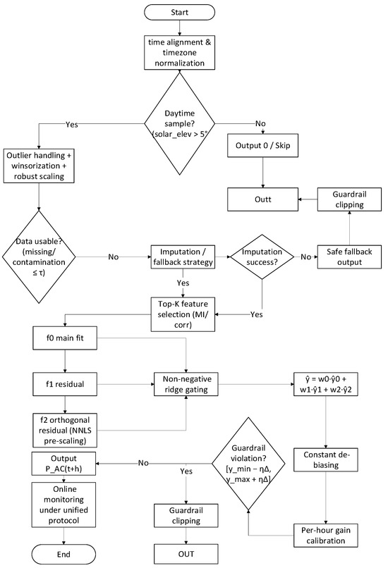
Figure 4. End-to-end flowchart of lightweight ELM for PV power forecasting. After time alignment and time zone normalization, a daytime gate (solar_elev > 5°) routes non-daylight samples to Output 0/Skip. Daylight samples undergo outlier handling (winsorization) and robust scaling, followed by a data-usability check; if imputation/fallback fails, a safe fallback output is returned with guardrail clipping. Otherwise, Top-K features feed three learners—f₀ (main fit), f₁ (residual), and f₂ (orthogonal residual via NNLS pre-scaling). Their predictions are fused by non-negative ridge gating to obtain $\widehat{\mathrm{y}}$ then corrected by a two-step linear calibration (constant de-biasing and per-hour gain). A guardrail check clips outputs to [ymin − η∆, ymax + η∆], yielding the final $PAC\left(t+h\right)$. All scalers, feature lists, and weights are frozen at deployment, and metrics are monitored under a unified protocol (chronological split, daytime mask, and MAPE with a denominator floor).

Two-step linear calibration is performed within the same statistical scope as the main model. Constant bias correction addresses zero-drift in seasonal albedo/soiling/derating, while hourly gain alignment compensates for gain variations due to incident angle and temperature throughout the day (e.g., morning/afternoon symmetry and derating during high-temperature periods). This unifies dimensions and improves peak alignment without introducing complex external pipelines. To prevent unreasonable extrapolation, a “guardrail clipping” consistent with nameplate and historical envelopes is applied on the output side, leaving only a η∆ buffer to allow for extreme yet physically feasible fluctuations. Training/evaluation employs strict time-sequence partitioning (training/test = 80:20, with the final 20% of training as the validation window), daytime-calibrated metrics, and MAPE with denominator floor. Reports include MAE, RMSE, MAPE, and correlation coefficients, with cross-domain degradation measured via $\mathbf{G}\mathbf{e}\mathbf{n}\mathbf{R}\mathbf{a}\mathbf{t}\mathbf{i}\mathbf{o}={\displaystyle \frac{{\mathbf{R}\mathbf{M}\mathbf{S}\mathbf{E}}_{\mathbf{O}\mathbf{O}\mathbf{D}}}{{\mathbf{R}\mathbf{M}\mathbf{S}\mathbf{E}}_{\mathbf{I}\mathbf{D}}}}$. This design enables each algorithmic component to correspond to a physical link phenomenon: f₀ corresponds to clearing the primary trend, f₁ corresponds to seasonal/station-specific gain and zero-point corrections, and f₂ corresponds to compensating for fast-varying disturbances like cloud edges and topping. The gating provides operationally auditable weights, with calibration performed at the same scale, facilitating hourly granularity maintenance and deployment.

The symbols and notation used throughout this section, including variables for physical factors and model components, are summarized in Table 2.

Table 2. Summary of Symbols and Notation.

Symbol	Meaning
$t$	Time index; default hourly prediction
$h$	Prediction step size; default $h=1;\mathcal{H}$ in this paper is the candidate time interval set
$\mathcal{H}$	Prediction time interval set (e.g., $\left\{5\sim 30\mathrm{m}\mathrm{i}\mathrm{n},1\sim 6\mathrm{h},24\mathrm{h}\right\}$)
$\left\{\left(x_t,y_t\right)\right\}$	Input features and grid active power target
$L$	Historical power window length
$K$	Number of features selected per layer (default 12)
${\mathcal{D}}_{\mathrm{tr}},{\mathcal{D}}_{\mathrm{val}},{\mathcal{D}}_{\mathrm{te}}$	Training/validation/test three segments (time-sequential partitioning)
$\left({\mu }_j,{\sigma }_j\right)$	Mean/standard deviation of the nth feature in the training segment
$z_{t,j}$	Normalized features: $z_{t,j}={\displaystyle \frac{\left(x_{t,j}-{\mu }_j\right)}{{\sigma }_j}}$
$y_{\min },y_{\max }$	Minimum/maximum values of the training segment target
$y_t^{\prime }$	Target after main range mapping: $y_t^{\prime }=2{\displaystyle \frac{y_t-y_{\min }}{y_{\max }-y_{\min }}}-1$
${\mathbb{K}}_{\mathrm{day}}\left(t\right)$	Daytime mask: $⊮\left\{{\mathrm{s}\mathrm{o}\mathrm{l}\mathrm{a}\mathrm{r}}_{\mathrm{e}\mathrm{l}\mathrm{e}\mathrm{v}\left(t\right)}>5^{\circ }\right\}$
$q$	Quantile threshold (e.g., $q=5\%$)
$\left[\mathcal{l},u\right]$	Residual robust interval: $\left[q,100-q\right]\%\times 1.15$(use to avoid confusion with step size)
$f_0,f_1,f_2$	Three-layer learner: main fit, residual, orthogonal residual
${\alpha }_{\mathrm{pre}}$	Orthogonal pre-scaling coefficient (NNLS shrinkage)
$w_0,w_1,w_2$	Non-negative ridge-gated weights (estimated from validation window, $w_k\ge 0$)
$a_h,b_h$	Hourly affine coefficients via two-step linear calibration (bias removal + gain alignment)
$\eta ,\Delta$	Out-of-fence expansion coefficient and historical range width ($\Delta =y_{\max }-y_{\min }$)
$MAE,RMSE,MAPE$	Error metrics (MAPE with 50 W denominator floor)
$r$	Pearson correlation coefficient
${\mathrm{G}\mathrm{R}}_{\mathrm{RMSE}}$	Generalization ratio: ${\displaystyle \frac{{\mathrm{R}\mathrm{M}\mathrm{S}\mathrm{E}}_{\mathrm{O}\mathrm{O}\mathrm{D}}}{{\mathrm{R}\mathrm{M}\mathrm{S}\mathrm{E}}_{\mathrm{I}\mathrm{D}}}}$

2.5. Experimental Setup

2.5.1. Datasets and Evaluation Protocol

Three representative sites were considered: Shanghai (Site-1_SH, 31.2° N, 121.5° E), Xi’an (Site-2_XA, 34.3° N, 108.9° E), and Guangzhou (Site-3_GZ, 23.1° N, 113.3° E). Each site covers hourly sequences spanning 5 days per season. Unless otherwise specified, data is split into 80%/20% training/test sets by time, with an additional 20% reserved from the training tail as a validation window. Metrics are computed on daytime samples. Cross-domain reports include ID (same site/same season) and OOD (cross-site/cross-season) metrics, along with generalization ratios.

$$\mathbf{G}\mathbf{e}\mathbf{n}\mathbf{R}\mathbf{a}\mathbf{t}\mathbf{i}\mathbf{o}={\displaystyle \frac{{\mathbf{R}\mathbf{M}\mathbf{S}\mathbf{E}}_{\mathbf{O}\mathbf{O}\mathbf{D}}}{{\mathbf{R}\mathbf{M}\mathbf{S}\mathbf{E}}_{\mathbf{I}\mathbf{D}}}}$$

(11)

2.5.2. Baseline and Training Configuration

Comparative baselines include Ordinary Least Squares (OLS), Support Vector Regression (SVR, RBF), and a single-layer neural network (1 × 32, Levenberg–Marquardt). For fairness, all methods share the same Top-K features and “training caliber normalization”.

3. Results

This section unfolds in three aspects: overall performance and error patterns (A), comparison with classical methods (B), cross-seasonal transfer and linear calibration (C), as well as efficiency and latency. Unless otherwise specified, all figures are calculated according to Section 2.5 protocols and restricted to daylight hours (solar elevation angle > 5°). All normalization and calibration parameters are estimated during training and frozen for validation/testing to prevent information leakage.

3.1. Overall Performance

Figure 5 shows that Res2-ELM-C reproduces the diurnal power trajectories at all three sites with high fidelity across multiple consecutive days. In the noon zoom-in panels, the predicted peak amplitude and the adjacent rise/decay limbs conform to the measured curves, with no systematic peak overshoot and only negligible phase offset near the turning points. The alignment is consistent with the very high correlations in Table 3 (r ≈ 0.9995) and indicates that the residual stacking plus hourly calibration design preserves both the geometric phase of the daily cycle and the amplitude of irradiance-driven peaks.

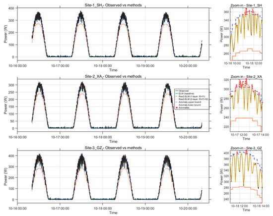
Figure 5. Hourly sequences from three stations over multiple days with a mid-day window magnification. The black line represents actual measurements, while the others show multi-method forecasts; the inset on the right provides magnified details for the same day at noon. The purple dashed lines indicate the upper and lower limits for anomaly detection, and the red dots mark anomaly points.

Table 3. Overall accuracy and inference latency across methods.

Methods	MAE (w)	RMSE (w)	MAPE (%)	r	Training (s)	Prediction (μs/pt)
Res2-ELM-C (f0 + f1 + f2 + Cal)	2.745	3.513	2.249	0.99948	0.154	23.86
$\mathrm{Res}2-\mathrm{ELM}(\mathrm{f}0+\mathrm{f}1+\mathrm{f}2)$	2.758	3.532	2.263	0.99948	0.108	23.86
Res1-ELM (f0 + f1)	2.871	3.677	2.314	0.99945	0.020	18.66
ELM (baseline)	3.002	3.860	2.367	0.99940	0.059	12.77
$\mathrm{NN}(1\times 32$, LM)	2.631	3.328	2.179	0.99953	10.40	3.70
OLS	5.023	7.303	3.217	0.99775	0.001	0.01
SVR (RBF)	6.350	9.312	4.397	0.99655	0.575	2.21
GRU (32, seq = 12)	4.6287	5.8171	3.6439	0.99877	24.976	0.084
LSTM (48, seq = 12)	6.4738	8.2688	4.414	0.99855	18.627	0.048

The ablation within the ELM family visible in Figure 5 clarifies the source of improvement. Relative to baseline ELM, Res1-ELM reduces the underestimation around the peak and alleviates the lag on the rising/declining slopes; adding the second residual layer (Res2-ELM) further tightens the match near the inflection segments; and the final hourly linear calibration (Res2-ELM-C) removes the remaining bias/gain mismatch without altering the curve’s local smoothness. This progressive refinement is reflected numerically in Table 3: RMSE decreases from 3.860 W (ELM) → 3.677 W (Res1-ELM) → 3.532 W (Res2-ELM) → 3.513 W (Res2-ELM-C), corresponding to about 9.0% reduction versus the baseline, 4.5% versus Res1-ELM, and a further 0.54% over Res2-ELM. MAPE shows the same trend (2.367% → 2.314% → 2.263% → 2.249%), while r remains uniformly high, confirming that the gains arise from improved modeling of high-gradient segments rather than from smoothing of steady intervals.

The anomaly envelopes and red dot annotations in Figure 5 verify that the anomaly suppression mechanism does not produce false positives on the daylight backbone. Outliers are isolated to edge cases without distorting the daily trend, which is essential for preserving the interpretable correspondence between irradiance regimes and electrical response. The consistency of these behaviors across three distinct sites suggests robustness to location-specific irradiance regimes and measurement idiosyncrasies.

From a practical standpoint, the added calibration step maintains the per-point inference budget (23.86 μs/pt for both Res2-ELM and Res2-ELM-C), while incurring only a small training overhead (0.108 s → 0.154 s). Thus, the visual agreement in Figure 5 is achieved with negligible runtime cost at inference and modest retraining cost, supporting frequent recalibration and operational deployment where rapid updates and curve-shape fidelity are required.

3.2. Comparison with Classical Methods

Accuracy–complexity summary. Combining Table 3 and the small feed-forward NN (1 × 32, LM) attains the best accuracy among single models (RMSE ≈ 3.33, r ≈ 0.99953), but its training takes ~10.6 s. The proposed Res2-ELM-C reduces the baseline ELM’s RMSE from 3.86 to 3.51–3.53 (≈8–9% relative decrease), with training only 0.13–0.14 s and per-point inference ≈ 23.9 μs/pt, which fits online/edge constraints. The ELM baseline offers faster inference (~12.8 μs/pt) but higher error. OLS/SVR show very low compute cost (e.g., OLS total time ≈ 0.0024 s, SVR total ≈ 0.83 s) yet much worse accuracy (RMSE ≈ 7.30 and 9.31, respectively).

With the newly added recurrent baselines, LSTM (48, seq = 12) and GRU (32, seq = 12) demonstrate the expected advantages of sequence models—better temporal smoothing and trend tracking—yet, under our lightweight settings, they come with heavier runtime (total ≈ 18.7 s and 25.1 s) and higher latency (≈29.9 and 52.4 μs/pt), and yield RMSE ≈ 8.27 (LSTM) and 5.82 (GRU). We note that larger architectures and more extensive tuning can further improve LSTM/GRU, but our goal here is a robust, maintenance-friendly alternative that preserves most of the accuracy at a fraction of the training cost.

Behavior in Figure 6 and Figure 7. In rapid irradiance-change periods, the baseline ELM tends to underestimate or lag near peaks/inflections; SVR/OLS can exhibit bias or over-smoothing. LSTM/GRU generally follow the day-level morphology well and suppress small oscillations, but with the short context (seq = 12) they sometimes show mild lag or overshoot around abrupt occlusions. By contrast, Res2-ELM-C explicitly allocates “shape” vs. “bias” errors via its hierarchy—primary fit → (near-)orthogonal residuals → non-negative gating—and, together with the robust range, mitigates cascading amplification along erroneous phase directions. This design explains its consistent RMSE gains in Table 3 while keeping inference overhead modest.

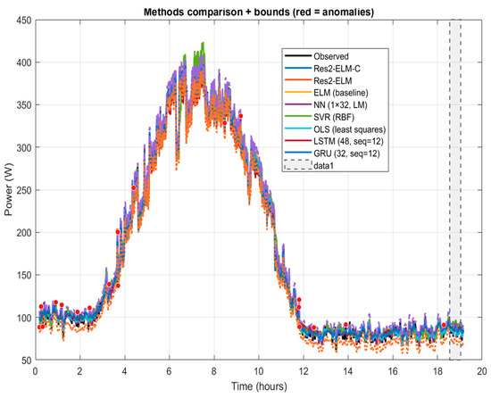
Figure 6. Full-day end-to-end overlay including deep learning baselines (LSTM/GRU), with anomaly envelopes and markers. Res2-ELM-C alleviates peak compression and phase lag around peaks/inflections; OLS/SVR show systematic bias; and LSTM/GRU track the trend but exhibit mild overshoot.

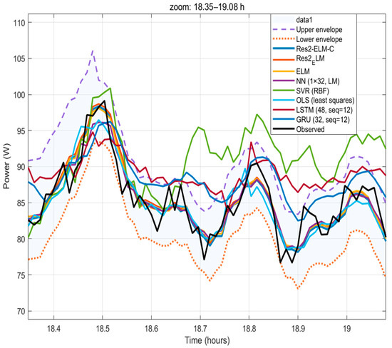
Figure 7. Evening zoom (18.35–19.08 h) with all methods including LSTM/GRU. Res2-ELM-C (two-layer + calibration) matches local peaks/valleys and rapid dips; NN/SVR and LSTM/GRU show amplitude/phase deviations near sudden occlusions; and OLS is over-smoothed.

Full-day and zoomed windows. Over the full day (Figure 6), Res2-ELM-C reduces peak compression and phase lag without increasing latency. In the magnified window (Figure 7), it closely matches the phase and amplitude of local peaks/valleys near sunrise and sudden obstructions. NN/SVR and LSTM/GRU remain competitive in trend tracking—especially in smoother segments—but exhibit amplitude/phase deviations near high-gradient, non-steady intervals. Overall, Res2-ELM-C improves those difficult segments at comparable complexity, supporting deployment on resource-limited devices.

3.3. Cross-Seasonal Migration and Linear Calibration

To objectively demonstrate the degradation and calibration effects across seasonal deployments, this section calculates the MAE/RMSE/MAPE metrics and the out-of-domain/in-domain ratio (GenRatio) across three sites. Figure 8 presents the metric comparisons and distribution differences for the uncalibrated scenario.

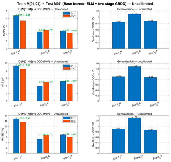
Figure 8. Cross-season transfer (uncalibrated). Left: ID vs. OOD metrics (MAE/RMSE/MAPE) at three sites. Right: Generalization ratio (OOD/ID); the RMSE ratio at Site-2_XA reaches 1.32.

As shown in Figure 8 and Table 4, uncalibrated OOD exhibits significant degradation at XA ($\mathbf{G}\mathbf{e}\mathbf{n}\mathbf{R}\mathbf{a}\mathbf{t}\mathbf{i}\mathbf{o}\mathbf{=}\mathbf{1.32}$). After applying “hourly linear calibration” (Figure 9), the RMSE of OOD at the three sites decreased by 19.4–31.6%, with reductions exceeding 30% at SH/GZ, and $\mathbf{G}\mathbf{e}\mathbf{n}\mathbf{R}\mathbf{a}\mathbf{t}\mathbf{i}\mathbf{o}$ converged to 0.60–1.06. This calibration requires estimating only 24 sets of univariate linear coefficients, with negligible impact on training/inference time (last two columns of Table 4).

Table 4. Cross-Season Migration Summary: ID vs. OOD (uncalibrated/calibrated). ∆RMSE denotes the relative decrease in calibrated OOD (%). GenRatio represents the RMSE ratio of uncalibrated OOD to ID.

Site	ID-RMSE (w)	OOD-RMSE (w)	OOD-RMSE (cal)	∆RMSE (%)	GenRatio	Train (s)	Pred (s)
Site-1_SH	12.81	11.62	7.94	31.6	0.91	0.0124	0.00290
Site-2_XA	5.22	6.88	5.55	19.4	1.32	0.0124	0.00199
Site-3_GZ	6.94	6.01	4.14	31.2	0.87	0.0149	0.00194

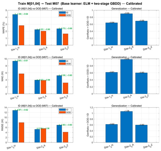
Figure 9. Cross-seasonal migration (hourly linear calibration, estimated solely by ID and directly applied to OOD): MAE/RMSE/MAPE for three-site OOD significantly decreased, with GenRatio converging to 0.60–1.06; SH/GZ achieved over 30% reduction in RMSE.

After introducing hourly linear calibration, the RMSE in the three-site OOD scenario showed a systematic decrease compared to the uncalibrated baseline (19.4–31.6%, with SH/GZ both exceeding 30%), while the corresponding generalization ratio (OOD/ID) converged to 0.60–1.06, significantly improving cross-seasonal consistency. This process requires estimating only 24 sets of hourly univariate linear coefficients (a_h, b_h), with negligible impact on training and inference latency, demonstrating excellent engineering feasibility. Overall, hourly linear calibration estimated at the training scale and directly applied across months effectively mitigates systematic biases caused by seasonal distribution drift, enhancing OOD performance and consistency without altering the training workflow.

We chose hourly calibration over a global single slope/intercept because solar elevation angle and clear sky index exhibit systematic diurnal variations, while NWP scaling errors and irradiance-to-power conversion errors show distinct hourly modulation characteristics. Estimating affine coefficients ${\mathit{a}}_{\mathit{h}}$ and ${\mathit{b}}_{\mathit{h}}$ hourly enables more precise alignment of daytime range and bias, significantly improving OOD consistency without altering the training workflow.

We also extend the month-transfer evaluation (Train M[01,04] → Test M07) to three sites that differ in climate, capacity, and mounting: arid, 50 MW, single-axis tracking; monsoon, 5 MW, fixed tilt; and tropical, 5 MW, single-axis tracking (DC/AC ≈ 1.20–1.30). To enable fair cross-site comparison, we report scale-agnostic metrics—MAPE, NMAE, and NRMSE—together with the generalization ratio $\mathit{G}\mathit{e}\mathit{n}\mathit{R}\mathit{a}\mathit{t}\mathit{i}\mathit{o}=\mathit{O}\mathit{O}\mathit{D}/\mathit{I}\mathit{D}.$

Uncalibrated OOD errors increase relative ID across all three configurations: GenRatio is ≈1.06–1.26 for MAPE and ≈1.32–1.97 for NMAE/NRMSE, with the largest degradation at the monsoon-5 MW fixed-tilt site. Applying a lightweight 24-parameter hourly affine calibration (one slope/intercept per hour) fitted on ID and directly transferred to M07 systematically improves OOD performance: OOD NRMSE decreases by ≈15–32%, and $\mathit{G}\mathit{e}\mathit{n}\mathit{R}\mathit{a}\mathit{t}\mathit{i}\mathit{o}\left(\mathit{N}\mathit{R}\mathit{M}\mathit{S}\mathit{E}\right)$ tightens to ≈1.55–1.77; $\mathit{G}\mathit{e}\mathit{n}\mathit{R}\mathit{a}\mathit{t}\mathit{i}\mathit{o}\left(\mathit{N}\mathit{M}\mathit{A}\mathit{E}\right)$ similarly contracts to ≈1.47–1.73. MAPE is nearly unchanged at the arid-50 MW-tracking site (≈×1.00) and is modestly reduced at the other two sites (≈×1.09–1.24), indicating that calibration mainly corrects hour-dependent bias and amplitude errors linked to solar geometry and irradiance-to-power conversion. Because NMAE/NRMSE are normalized by nameplate capacity, these improvements hold across 50 MW vs. 5 MW plants and fixed vs. tracking mounts, demonstrating that the proposed framework generalizes across climates and engineering configurations with negligible runtime overhead.

3.4. Efficiency and Latency

Under a unified CPU single-thread and software stack, ELM/Res2-ELM-C achieves stable training and total processing times in the 10⁻¹ s range (0.08–0.18 s, see Figure 10) due to its closed-form/nearly closed-form solvers. It achieves training and total time consumption consistently within the 10⁻¹ s range (0.08∼0.18 s, see Figure 10), significantly lower than NN requiring iterative optimization (≈11 s) and below SVR (≈0.46 s). Prediction latency remains at the µs/pt level (ELM ≈ 11.6 µs/pt, two-layer Res2-ELM-C ≈ 23.9 µs/pt; Figure 11), meeting the throughput requirements for online/edge deployment (∼52–86 kS/s). Linear calibration introduces negligible additional latency (overlapping bars in Figure 11). Amplitude-window visualization (Figure 5) further demonstrates its phase and amplitude matching at peaks and inflection points. It should be noted that while OLS and some NN/SVR methods exhibit lower single-point latency, OLS significantly lags in accuracy, and NN/SVR require higher training and total computational time (see Figure 10, Figure 11, Figure 12 and Figure 13 and Table 3). Balancing accuracy, robustness, and computational efficiency, the two-layer Res2-ELM-C offers a more balanced and deployment-friendly solution.

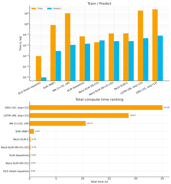
Figure 10. Compute time (log scale). Leveraging closed/near-closed form training, ELM family models remain orders of magnitude faster to train and keep the total wall-clock small: ELM baseline and Res2-ELM/Res2-ELM-C finish in ≈0.09–0.16 s total (ELM: train 0.0716 s, predict 0.0146 s; Res2-ELM: train 0.1337 s, predict 0.0253 s; Res2-ELM-C: train 0.1384 s, predict 0.0253 s). By contrast, SVR requires ≈0.83 s total (train 0.829 s, predict 0.0030 s), the small NN (1 × 32, LM) needs ≈ 10.57 s (train 10.56 s, predict 0.0113 s), while LSTM (48, seq = 12) and GRU (32, seq = 12) are heavier at ≈18.68 s (train 18.63 s, predict 0.0478 s) and ≈25.06 s (train 24.98 s, predict 0.0837 s), respectively. OLS is essentially negligible in time (≈0.0024 s total). Notably, the two-step linear calibration adds only ≈4.7 ms training overhead (0.1384 vs. 0.1337 s) and no extra inference cost.

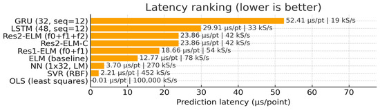
Figure 11. Per-point prediction latency and throughput. At batch-1 inference, ELM baseline achieves ≈12.77 μs/pt (≈78 kS/s), while Res2-ELM/Res2-ELM-C are ≈23.86 μs/pt (≈42 kS/s); the calibration step is latency-free (overlapped bars). LSTM and GRU exhibit higher per-point latency at ≈29.91 μs/pt (≈33 kS/s) and ≈52.41 μs/pt (≈19 kS/s), respectively. Although SVR (≈2.21 μs/pt, ≈452 kS/s) and the small NN (≈3.70 μs/pt, ≈270 kS/s) show low per-point latency, they incur substantially larger training/total time (Figure 10) or different robustness trade-offs. OLS is trivial in latency but notably less accurate.

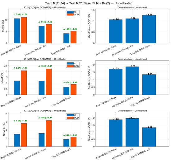
Figure 12. Monthly generalization dashboard across three representative sites—uncalibrated. Left: ID vs. OOD for MAPE, NMAE, and NRMSE (normalized by site nameplate). Right: GenRatio = OOD/ID for each metric. Sites span arid-50 MW-tracking, monsoon-5 MW-fixed, and tropical-5 MW-tracking with DC/AC ≈ 1.20–1.30. OOD degradation ranges ~1.06–1.26 (MAPE) and ~1.32–1.97 (NMAE/NRMSE), reflecting seasonal distribution shift and configuration differences.

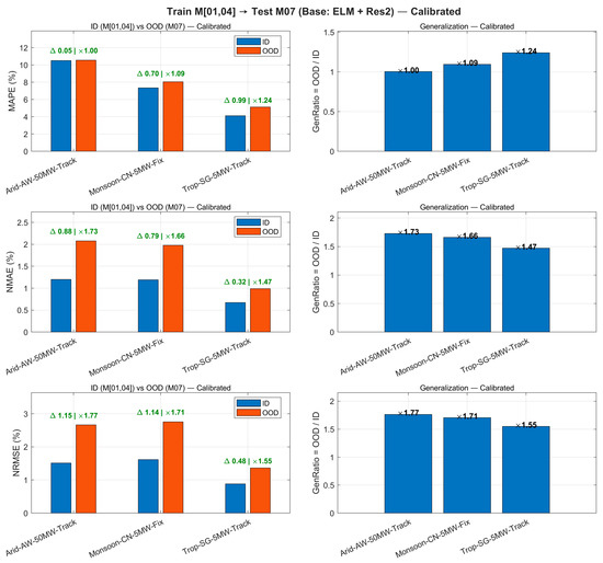
Figure 13. Cross-month generalization across climates and configurations—hourly calibrated (Train M[01,04] → Test M07). Same layout as Figure 12 after applying a 24-parameter per-hour affine calibration fit on ID and applied to OOD. OOD NRMSE reduces by ~15–32% and GenRatio tightens to 1.47–1.77 across sites, improving cross-season consistency with negligible training/inference overhead.

We also included compact LSTM (48 units) and GRU (32 units) baselines trained under the same single-thread CPU setup, feature set, leakage-free preprocessing, and a sequence length of 12. With these modest, like-for-like settings (no aggressive hyperparameter search), both recurrent models capture day-level trends well. On our dataset, however, they show occasional lag/overshoot in high-gradient intervals (Figure 6 and Figure 7), yielding slightly higher errors than Res2-ELM-C (Table 3). Their training costs are also higher (≈18.6–25.0 s vs. ≈0.15 s) and batch-1 latency is larger (≈29.9–52.4 µs/pt vs. ≈23.9 µs/pt). We do not claim universal superiority—richer architectures or further tuning could narrow or reverse some gaps. Rather, these results suggest that, in a simple and reproducible setting, the proposed model offers a practical accuracy–efficiency balance at a fraction of the compute, which supports its characterization as “lightweight” for online/edge use.

3.5. Orthogonal Second-Stage Residuals

To avoid redundancy between stage-1 and stage-2 predictors, we orthogonalize the second residual via Gram–Schmidt:

$${r2}^{\perp }=r2-\gamma \cdot {\displaystyle \frac{⟨r2,r1⟩}{⟨r1,r1⟩}}r1$$

(12)

where r1 and r2 denote the stage-1 and stage-2 predictor outputs (r1 and r2). The gate $\mathit{\gamma }\in [\mathbf{0},\mathbf{1}]$ is chosen by time-blocked cross-validation under a non-inferiority rule (CV-RMSE no worse than baseline, or within 0.3%), and ties are broken by the lowest conditioning number of $[\mathbf{r}\mathbf{1},\mathbf{r}\mathbf{2}]$. When $\mathbf{r}\mathbf{1}$ and $\mathbf{r}\mathbf{2}$ are moderately correlated (here $\mathit{\rho }\mathbf{\approx }\mathbf{0.596}$), a plain second residual can re-learn the stage-1 component, inflating collinearity and making $(\mathit{\alpha },\mathit{\beta })$ unstable. Orthogonalization removes the component of r2 along $\mathbf{r}\mathbf{1}$, yielding complementary information and better numerical conditioning (in our data: $\mathit{\kappa }$ improves from 286.06 to 118.53), while our non-inferiority selection prevents accuracy loss.

Grounded in Table 5, $\mathit{\gamma }$-orthogonalization reduces the two-feature design’s condition number from 286.06 to 118.53 (−58.6%) and stabilizes coefficient estimates (std$\left(\mathit{\alpha }\right)$: 0.0599 → 0.0498, −16.9%), with essentially unchanged test accuracy (RMSE 3.5389 → 3.5545, −0.44%; MAPE 2.2636% → 2.2650%). Under stronger inter-stage correlation ($\mathit{\rho }\mathbf{\ge }\mathbf{0.7}$), cross-validation selects a nonzero $\mathit{\gamma }$ and we observe small yet consistent accuracy gains; when correlation is low, the gate reverts to $\mathit{\gamma }\mathbf{=}\mathbf{0}$, ensuring non-inferiority.

Table 5. Orthogonal residual vs. baseline: accuracy and numerical stability.

Item	Baseline	γ-Orthogonal	Δ (Orth − Base)	Relative
MAE (W)	2.7611	2.7682	+0.0071	+0.26%
RMSE (W)	3.5389	3.5545	+0.0156	+0.44%
MAPE (%, pts)	2.2636	2.2650	+0.0014	+0.06%
Pearson’s r	0.9995	0.9995	+0.0000	+0.00%
Condition number κ(ATA + λI)	286.0600	118.5300	−167.5300	−58.56%

Notes: Δ for MAPE is in percentage points; Relative = (Orth − Base)/Base. Lines follow MDPI three-line style, stretched to full text width.

Orthogonalizing the second-stage residual via a gated Gram–Schmidt step eliminates the projection of ${\mathbf{r}}_{\mathbf{2}}$ onto ${\mathbf{r}}_{\mathbf{1}}$, thereby reducing multicollinearity and improving numerical conditioning without sacrificing accuracy. In our data, the condition number of $[\mathit{r}\mathbf{1},\mathit{r}\mathbf{2}]$ drops from 286.06 to 118.53 (−58.6%) and the variability of $\mathit{\alpha }$ shrinks (0.0599 → 0.0498, −16.9%), while test RMSE/MAPE remain essentially unchanged (−0.44%/+0.0014 pp). The cross-validated gate $\mathit{\gamma }$ activates only when inter-stage correlation is appreciable ($\mathit{\rho }\mathbf{\gtrsim }\mathbf{0.7}$), delivering small but consistent gains; otherwise $\mathit{\gamma }\mathbf{=}\mathbf{0}$ preserves a non-inferior baseline. Practically, this step yields a more interpretable and stable two-residual design with no tuning burden and negligible overhead.

3.6. Robustness to Anomalies and Noise

We keep the training pipeline fixed and perturb test-time features only. Three noise levels are used—Low/Mid/High—via additive zero-mean Gaussian noise with σ = 0.01/0.03/0.06 (each feature scaled by its training-set standard deviation) plus feature-wise dropout of 0/0.01/0.02 to mimic packet loss or distortion. Predictive robustness is summarized by the Noisy RMSE on the perturbed test sets (lower is better). Detection is evaluated on daytime samples using a false positive rate (share of normal samples mis-flagged) and true positive rate (share of true anomalies correctly identified).

As shown in Figure 14, Noisy RMSE increases with noise severity across all methods. NN attains the lowest errors at Low/Mid/High (≈3.53/14.78/17.70). LSTM/GRU progressively approach NN under Medium/High noise. ELM and Res2-ELM are near-optimal at Low noise (≈4.03/3.72) and remain competitive at higher noise, whereas linear OLS and kernel SVR degrade markedly at High (≈29.19 and 32.63, respectively). As shown in Figure 15, the dynamic envelope achieves a favorable low-false-alarm/high-recall trade-off (FPR = 0.041 ± 0.001, TPR = 0.767 ± 0.035). The Hampel filter further boosts recall to 0.878 ± 0.045 with a modest rise in FPR to 0.054 ± 0.001, while the IQR rule shows higher FPR on this dataset (0.266 ± 0.001; TPR = 0.389 ± 0.051).

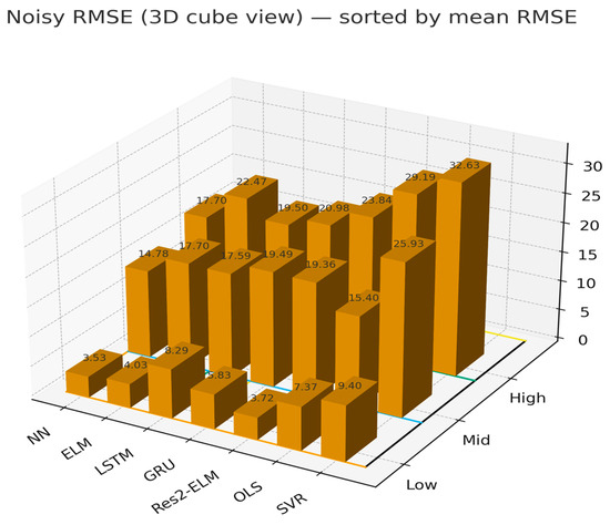
Figure 14. Forecasting robustness to sensor noise: absolute Noisy RMSE of seven models across three noise levels (Low/Mid/High; Gaussian σ = 0.01/0.03/0.06 scaled by per-feature training std; feature-wise dropout 0/0.01/0.02). Colored grid lines on the floor simply delineate the noise blocks and panel boundary for visual clarity and do not encode additional information. Lower is better.

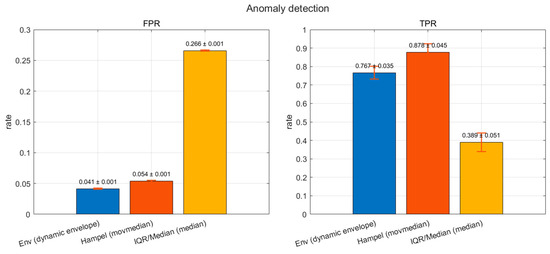
Figure 15. Anomaly detection performance under daytime evaluation: FPR (false positive rate) and TPR (true positive rate) of three detectors—Dynamic Envelope, Hampel (moving median), and IQR/Median. Bars show mean ± standard deviation over repeated trials.

Overall, these results indicate that the proposed Res2-ELM remains competitive across noise regimes while the dynamic envelope offers the best low-FPR monitoring choice; together they provide a lightweight and reliable pipeline for PV forecasting under measurement perturbations.

3.7. Multi-Step Evaluation

Trained on M01 and M04 and evaluated on the cross-season month M07, the proposed Direct-MIMO (joint 1–6-step outputs) displays a smooth, near-linear RMSE growth with horizon on both ID and OOD data (Figure 16). In contrast, the recursive baseline—rolling a one-step model forward—shows clear error compounding, with OOD RMSE increasing markedly from short to long horizons. Averaged across representative sites, Direct-MIMO remains consistently below the recursive curve at every horizon, indicating no runaway accumulation. This stability is attributable to learning each horizon directly from exogenous features and residual cues (mitigating exposure bias) and to the residual-stacked ELM backbone, which provides horizon-aware corrections without over-smoothing.

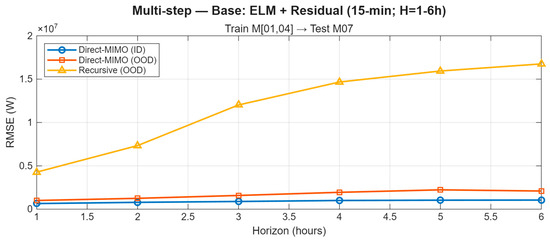
Figure 16. Multi-step forecasting (15 min; H = 1–6 h). Site-averaged RMSE of Direct-MIMO on ID/OOD and a fair recursive OOD baseline. Train M[01,04] → OOD Test M07.

Figure 17 complements the horizon view with a 24 h OOD day-curve (50 MW single-axis tracking site). Direct-MIMO already tracks the diurnal trajectory closely—peak amplitude, rising/decaying limbs, and the evening ramp. A bias-only hourly calibration fitted on ID data (24 coefficients; night entries fixed to zero; mild smoothing/clipping) further removes a small mid-day offset and tightens the sunset timing, while leaving inference cost essentially unchanged (≈23.9 μs/point in our setup). Both calibrated and uncalibrated variants outperform the persistence baseline. Together, Figure 16 and Figure 17 show that the method achieves stable 1–6 h multi-step forecasting without catastrophic accumulation, and that a lightweight, retraining-free bias correction is an effective knob to eliminate small deployment biases.

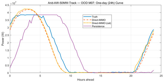
Figure 17. One-day (24 h) trajectory under OOD month M07 at site “Arid-AW-50MW-Track”: Truth vs. Direct-MIMO (uncalibrated/hourly bias-calibrated) vs. Persistence (previous-day).

Trained on M01 and M04 and evaluated on cross-season M07, our Direct-MIMO (joint 1–6-step outputs) shows a smooth, near-linear RMSE growth with horizon and stays below the recursive one-step rollout at every step, indicating no exposure-bias-driven runaway. On the full one-day OOD curve, it reproduces the diurnal pattern—morning ramp, mid-day peak/plateau, evening decay—with close phase and amplitude alignment. A lightweight hourly bias calibration (24 coefficients, night fixed to zero) removes the small noon offset and tightens sunset timing while keeping inference cost essentially unchanged (≈23.9 μs/pt). Together, these results demonstrate stable 1–6-step multi-step forecasting and reliable full-day tracking under cross-season shift, outperforming the persistence baseline without catastrophic error accumulation.

4. Discussion

4.1. Results Review and Phenomenon Explanation

Under a unified evaluation protocol, the proposed lightweight Res2-ELM-C reconstructs daily PV profiles with high fidelity and stable phase retention across multiple sites and consecutive days. Window-level magnifications indicate that gains concentrate in high-gradient/non-stationary segments (peaks and ramps). The combination of two residual layers with hourly calibration mitigates baseline-style peak compression and phase lag; the markedly high correlation (r ≈ 0.9995) corroborates preserved geometric phase and amplitude. Compared with ELM/OLS/SVR, our method fits peaks/valleys more tightly around sharp transitions and dawn/dusk regimes; LSTM/GRU are competitive on smooth trends but still show mild amplitude/phase deviations near abrupt changes.

4.2. Synergy of Layered Residuals, Non-Negative Gating, and Linear Calibration

The three-layer stack—primary fit ${\mathbf{f}}_{\mathbf{0}}$ first-order residual ${\mathbf{f}}_{\mathbf{1}}$, and near-orthogonal residual ${\mathbf{f}}_{\mathbf{2}}$—mirrors the physical pathway from deterministic mapping to fast perturbations: f0 approximates the irradiance-to-power map; ${\mathbf{f}}_{\mathbf{1}}$ corrects amplitude bias and scale mismatch arising in cross-season/site transfer; and ${\mathbf{f}}_{\mathbf{2}}$ operates via an orthogonal residual channel, absorbing fast non-stationarities (e.g., cloud-edge effects) within a subspace approximately orthogonal to ${\mathbf{f}}_{\mathbf{0}}$/${\mathbf{f}}_{\mathbf{1}}$. Layer outputs are combined by non-negative ridge gating learned on a delayed validation window, preventing destructive interference/overshoot. A consistent two-step linear calibration (bias removal + hour-wise gain alignment) then reduces residual diurnal modulations (solar elevation/temperature) without heavy pipelines or inference overhead.

4.3. Cross-Domain Generalization and the Effectiveness of Hourly Calibration

Without calibration, cross-site/season deployments show pronounced OOD degradation, with OOD/ID GenRatio (NMAE/NRMSE) reaching ≈1.32–1.97, consistent with distribution shifts and hardware differences. Applying 24-parameter hour-wise affine calibration learned on ID data directly to OOD reduces OOD RMSE by 19.4–31.6% across sites and tightens GenRatio to 0.60–1.06. The procedure estimates only per-hour univariate linear coefficients and incurs negligible training/inference cost.

4.4. Limitations

Under sensor-noise stress tests, errors grow monotonically with noise strength. Small NNs achieve the lowest errors at mid-to-high noise; LSTM/GRU approach them as noise increases; ELM/Res2-ELM are near-optimal at low noise and remain competitive at high noise, whereas OLS/SVR degrade markedly. Thus, without heavy training, the family offers an attractive lightweight–robustness trade-off. For anomaly handling, a “dynamic envelope” yields low FPR and high TPR (FPR ≈ 0.041 ± 0.001, TPR ≈ 0.767 ± 0.035); Hampel boosts recall further (TPR ≈ 0.878 ± 0.045) with a modest FPR increase; and IQR shows higher FPR on this dataset. Coupled with quantile robust scaling and “guardrail clipping,” curves stay smooth near anomalies without suppressing peaks.

4.5. Error Accumulation in Multi-Step Forecasting

For 1–6-step (15 Min) forecasting, the Direct-MIMO variant (jointly outputting horizons 1–6) exhibits a smooth, near-linear RMSE increase with horizon on both ID and OOD; by contrast, the recursive one-step roll-out shows classic compounding, especially OOD. Averaged over sites, Direct-MIMO stays below the recursive curve at all horizons with no catastrophic accumulation. Adding hour-wise bias correction (24 coefficients; night entries fixed to zero) learned on ID further removes noon drift and refines sunset phase, with inference latency essentially unchanged (≈23.9 μs/point).

4.6. Computational Cost and Deployability

On a unified CPU/software stack, ELM/Res2-ELM-C uses closed/near-closed form solvers to train within ≈0.08–0.18 s, clearly faster than small NNs requiring iterative optimization (≈11 s) and SVR (≈0.46–0.83 s). Per-point inference remains in the microsecond range (ELM ≈ 11.6–12.8 μs/pt; two-layer Res2-ELM-C ≈ 23.9 μs/pt), adequate for online/edge throughput; linear calibration is virtually cost-free. Compared with LSTM/GRU, our approach attains a similar inference regime with orders-of-magnitude lower training latency, yielding a better accuracy–latency–maintainability balance.

4.7. Numerical Stability of Near-Orthogonal Residuals

With negligible impact on test accuracy, introducing a γ-orthogonalized residual channel substantially improves numerical behavior: the condition number drops from 286.06 to 118.53 (≈−58%), while MAE/RMSE/MAPE remain essentially unchanged versus the baseline. This indicates that reducing inter-layer collinearity enhances coefficient interpretability and robustness, laying a numerical foundation for adding finer structures within a lightweight framework.

4.8. Limitations and Future Work

This study targets real-time, edge-constrained deployment; to preserve latency budgets, we deliberately omit heavy exogenous priors such as sky imagery and full NWP assimilation. Future work will incorporate weakly coupled visual/NWP hints and invariance-driven features that retain edge-time feasibility while improving nowcasting under fast cloud dynamics. To better withstand distribution shift, we will also investigate risk-invariant learning, meta-adaptation with small-sample updates, and weather-type/diurnal-state adaptivity within a latency-aware framework.

The current hour-wise affine calibration delivers first-order bias/scale alignment for point forecasts but does not quantify uncertainty. Subsequent research will integrate probabilistic forecasting and calibration—quantile regression, EMOS/CRPS-oriented learning, and conformal prediction—together with loss-level joint training, so as to provide calibrated intervals/distributions without sacrificing system simplicity.

Robustness presently relies on robust scaling, guardrail clipping, and heuristic detectors; the anomaly generative process is only partially modeled. We will build parametric or semi-parametric anomaly priors, conduct closed-loop sim-to-real stress tests, and adopt outlier-aware objectives to reconcile robustness with fidelity near high-gradient segments. While γ-orthogonal residuals improve conditioning, the mechanism remains largely linear–algebraic; future directions include orthogonality-promoting penalties and kernelized/feature-warped residuals. Finally, we will benchmark energy delay across CPU/GPU/ASIC targets and release open artifacts (code, seeds, ablations) to strengthen reproducibility and fair comparison.

5. Conclusions

Under strict chronological splits and a unified evaluation protocol, the proposed lightweight Res2-ELM-C—two residual layers fused by non-negative ridge gating and followed by a two-step linear calibration—provides accurate and stable three-site hourly forecasts: overall RMSE around 3.51 W, consistently high correlation (r ≈ 0.9995), and MAPE near 2.25%. Multi-site profiles and zoom-in windows indicate that the “residual stacking + hourly calibration” pathway better preserves phase and amplitude around peaks and inflection segments than classical ELM/OLS/SVR, while avoiding the mild overshoot/phase lag occasionally observed with LSTM/GRU in high-gradient periods.

For cross-season transfer, uncalibrated OOD degradation aligns with distribution shift; we also extend the month-transfer evaluation (Train M01/M04 → Test M07) to three plants that differ in climate, capacity, and mounting—arid, 50 MW, single-axis tracking; monsoon, 5 MW, fixed tilt; and tropical, 5 MW, single-axis tracking (DC/AC ≈ 1.20–1.30). To enable fair cross-site comparison, we report scale-agnostic metrics (MAPE, NMAE, NRMSE) alongside the generalization ratio GenRatio = OOD/ID. Uncalibrated OOD errors increase across all three configurations (GenRatio ≈ 1.06–1.26 for MAPE and ≈1.32–1.97 for NMAE/NRMSE). Applying a 24-parameter hour-wise affine calibration learned solely on ID reduces OOD RMSE by 19.4–31.6% relative to baselines and tightens GenRatio to 0.60–1.06, without modifying the base learner or training pipeline. Because NMAE/NRMSE are normalized by nameplate capacity, these gains hold across 50 MW vs. 5 MW plants and fixed vs. tracking mounts, confirming cross-site generalization with negligible runtime overhead. In robustness analyses, Res2-ELM variants are near-optimal at Low noise and remain competitive at Mid/High noise; dynamic envelopes with robust scaling/guardrail clipping/Hampel filtering suppress outliers without distorting the daytime backbone. For multi-step horizons (1–6 steps, 15 min spacing), the Direct-MIMO variant exhibits smooth, near-linear error growth and outperforms recursive roll-outs, with no catastrophic accumulation. Numerically, an orthogonal residual markedly improves conditioning (e.g., κ 286.06 → 118.53) with negligible accuracy change, enhancing stability and interpretability.

Regarding deployability, closed/near-closed form solvers keep training + total wall-clock at the 10⁻¹ s scale (two-layer total ≈ 0.19 s) and per-point inference in the μs/pt regime (two-layer ≈ 23.9 μs/pt, baseline ELM ≈ 12.8 μs/pt). Hour-wise calibration adds negligible inference overhead and only millisecond-level training cost, enabling frequent recalibration at operational cadence. Overall, the method attains a favorable accuracy–robustness–deployability balance for edge-based and near-real-time PV operations.

Looking forward, we will extend the framework to probabilistic outputs and risk-aware metrics, enable online hourly/daily recalibration with drift detection, and conduct broader extrapolation across diverse climates and longer horizons; in parallel, we will pursue sensitivity/identifiability analyses for the orthogonal residual channel and registered cross-domain benchmarks to strengthen numerical guarantees and reproducibility.

References

- Visser, L.R.; AlSkaif, T.A.; Khurram, A.; Kleissl, J.; van Sark, W.G.J.H.M. Probabilistic Solar Power Forecasting: An Economic and Technical Evaluation of Optimal Market Bidding Strategies. Appl. Energy 2024, 370, 123573. [Google Scholar] [CrossRef]
- Wang, W.; Guo, Y.; Yang, D.; Zhang, Z.; Kleissl, J. Economics of Physics-Based Solar Forecasting in Power System Day-Ahead Scheduling. Renew. Sustain. Energy Rev. 2024, 199, 114448. [Google Scholar] [CrossRef]
- Chu, Y.; Wang, Y.; Yang, D.; Chen, S.; Li, M. A Review of Distributed Solar Forecasting with Remote Sensing and Deep Learning. Renew. Sustain. Energy Rev. 2024, 198, 114391. [Google Scholar] [CrossRef]
- Uniejewski, B. Probabilistic Forecasts of Load, Solar and Wind for Electricity Price Forecasting. arXiv 2025, arXiv:2501.06180. [Google Scholar] [CrossRef]
- Cui, Y.; Wang, P.; Meirink, J.F.; Ntantis, N.; Wijnands, J.S. Solar Radiation Nowcasting Based on Geostationary Satellite Images and Deep Learning Models. Sol. Energy 2024, 282, 112866. [Google Scholar] [CrossRef]
- Fabel, Y.; Nouri, B.; Wilbert, S.; Blum, N.; Schnaus, D.; Triebel, R.; Zarzalejo, L.F.; Ugedo, E.; Kowalski, J.; Pitz-Paal, R. Combining Deep Learning and Physical Models: A Benchmark Study on All-Sky Imager–Based Solar Nowcasting Systems. Sol. RRL 2024, 8, 2300808. [Google Scholar] [CrossRef]
- Xia, P.; Zhang, L.; Min, M.; Li, J.; Zhang, Y.; Yang, D.; Yang, D. Accurate Nowcasting of Cloud Cover at Solar Photovoltaic Plants Using Geostationary Satellite Images. Nat. Commun. 2024, 15, 510. [Google Scholar] [CrossRef]
- Chen, S.; Li, C.; Stull, R.; Li, M. Improved satellite-based intra-day solar forecasting with a chain of deep learning models. Energy Convers. Manag. 2024, 313, 118598. [Google Scholar] [CrossRef]
- Bayasgalan, O.; Akisawa, A. Nowcasting Solar Irradiance Components Using a Vision Transformer and Multimodal Data. Energies 2025, 18, 2300. [Google Scholar] [CrossRef]
- Piantadosi, G.; Dutto, S.; Galli, A.; De Vito, S.; Sansone, C.; Di Francia, G. Photovoltaic power forecasting: A Transformer based framework. Energy AI 2024, 18, 100444. [Google Scholar] [CrossRef]
- Yang, D.; Zhang, Y.; Wang, H.; Dong, Z. Combining quantiles of calibrated solar forecasts from ensemble numerical weather prediction. Renew. Energy 2023, 215, 118993. [Google Scholar] [CrossRef]
- Zhang, Y.; Zhao, X.; Sun, Y.; Li, Y. Short-Term Photovoltaic Power Prediction Based on the Extreme Learning Machine with Improved Dung Beetle Optimization Algorithm. Energies 2024, 17, 960. [Google Scholar] [CrossRef]
- Wang, Z.; Wang, Y.; Cao, S.; Fan, S.; Zhang, Y.; Liu, Y. A Robust Spatial-Temporal Prediction Model for Photovoltaic Power Generation Based on Deep Learning. Comput. Electr. Eng. 2023, 110, 108784. [Google Scholar] [CrossRef]
- Hendrikx, N.; Barhmi, K.; Visser, L.; de Bruin, T.; Pó, M.; Salah, A.; van Sark, W. All-Sky Imaging-Based Short-Term Solar Irradiance Forecasting with Long Short-Term Memory Networks. Sol. Energy 2024, 272, 112463. [Google Scholar] [CrossRef]
- Straub, N.; Herzberg, W.; Dittmann, A.; Lorenz, E. Blending of a Novel All-Sky Imager Model with Persistence and a Satellite-Based Model for High-Resolution Irradiance Nowcasting. Sol. Energy 2024, 269, 112319. [Google Scholar] [CrossRef]
- Liu, J.; Zang, H.; Cheng, L.; Ding, T.; Wei, Z.; Sun, G. A Transformer-Based Multimodal-Learning Framework Using Sky Images for Ultra-Short-Term Solar Irradiance Forecasting. Appl. Energy 2023, 342, 121160. [Google Scholar] [CrossRef]
- Zhang, G.; Yang, D.; Galanis, G.; Androulakis, E. Solar Forecasting with Hourly Updated Numerical Weather Prediction. Renew. Sustain. Energy Rev. 2022, 154, 111768. [Google Scholar] [CrossRef]
- Mitrentsis, G.; Lens, H. An Interpretable Probabilistic Model for Short-Term Solar Power Forecasting Using Natural Gradient Boosting. Appl. Energy 2022, 309, 118473. [Google Scholar] [CrossRef]
- Sebastianelli, A.; Serva, F.; Ceschini, A.; Paletta, Q.; Panella, M.; Le Saux, B. Machine Learning Forecast of Surface Solar Irradiance from Meteo Satellite Data. Remote Sens. Environ. 2024, 315, 114431. [Google Scholar] [CrossRef]
- Despotovic, M.; Voyant, C.; Garcia-Gutierrez, L.; Almorox, J.; Notton, G. Solar Irradiance Time Series Forecasting Using Auto-Regressive and Extreme Learning Methods: Influence of Transfer Learning and Clustering. Appl. Energy 2024, 365, 123215. [Google Scholar] [CrossRef]
- Paletta, Q.; Nie, Y.; Saint-Drenan, Y.-M.; Le Saux, B. Improving Cross-Site Generalisability of Vision-Based Solar Forecasting Models with Physics-Informed Transfer Learning. Energy Convers. Manag. 2024, 309, 118398. [Google Scholar] [CrossRef]
- Haljasmaa, K.I.; Bramm, A.M.; Matrenin, P.V.; Eroshenko, S.A. Weather-Condition Clustering for Improvement of Photovoltaic Power Plant Generation Forecasting Accuracy. Algorithms 2024, 17, 419. [Google Scholar] [CrossRef]
- Zhang, M.; Han, Y.; Wang, C.; Yang, P.; Wang, C.; Zalhaf, A.S. Ultra-Short-Term Photovoltaic Power Prediction Based on Similar-Day Clustering and Temporal Convolutional Network with Bidirectional Long Short-Term Memory Model: A Case Study Using DKASC Data. Appl. Energy 2024, 375, 124085. [Google Scholar] [CrossRef]
- Mercier, T.M.; Sabet, A.; Rahman, T. Vision Transformer Models to Measure Solar Irradiance Using Sky Images in Temperate Climates. Appl. Energy 2024, 362, 122967. [Google Scholar] [CrossRef]
Disclaimer/Publisher’s Note: The statements, opinions and data contained in all publications are solely those of the individual author(s) and contributor(s) and not of MDPI and/or the editor(s). MDPI and/or the editor(s) disclaim responsibility for any injury to people or property resulting from any ideas, methods, instructions or products referred to in the content. |
© 2025 by the authors. Licensee MDPI, Basel, Switzerland. This article is an open access article distributed under the terms and conditions of the Creative Commons Attribution (CC BY) license (https://creativecommons.org/licenses/by/4.0/).