A Deep Neural Network-Based Approach for Optimizing Ammonia–Hydrogen Combustion Mechanism

Abstract

Ammonia is a highly promising zero-carbon fuel for engines. However, it exhibits high ignition energy, slow flame propagation, and severe pollutant emissions, so it is usually burned in combination with highly reactive fuels such as hydrogen. An accurate understanding and modeling of ammonia–hydrogen combustion is of fundamental and practical significance to its application. Deep Neural Networks (DNNs) demonstrate significant potential in autonomously learning the interactions between high-dimensional inputs. This study proposed a deep neural network-based method for optimizing chemical reaction mechanism parameters, producing an optimized mechanism file as the final output. The novelty lies in two aspects: first, it systematically compares three DNN structures (Multi-layer perceptron (MLP), Convolutional Neural Network, and Residual Regression Neural Network (ResNet)) with other machine learning models (generalized linear regression (GLR), support vector machine (SVM), random forest (RF)) to identify the most effective structure for mapping combustion-related variables; second, it develops a ResNet-based surrogate model for ammonia–hydrogen mechanism optimization. For the test set (20% of the total dataset), the ResNet outperformed all other ML models and empirical correlations, achieving a coefficient of determination (R²) of 0.9923 and root mean square error (RMSE) of 135. The surrogate model uses the trained ResNet to optimize mechanism parameters based on a Stagni mechanism by mapping the initial conditions to experimental IDT. The results show that the optimized mechanism improves the prediction accuracy on laminar flame speed (LFS) by approximately 36.6% compared to the original mechanism. This method, while initially applied to the optimization of an ammonia–hydrogen combustion mechanism, can potentially be adapted to optimize mechanisms for other fuels.

1. Introduction

Over the past decade, ammonia (NH₃) has attracted significant attention as a promising alternative fuel. Ammonia is primarily produced via the Haber–Bosch method, which operates under high temperatures and pressures, thus making it highly energy-consuming [1]. For the large-scale generation of oxygen, nitrogen, and argon, cryogenic air separation is recognized as the most efficient and cost-efficient approach [2]. Molybdenum complexes are capable of catalyzing nitrogen fixation under ambient conditions when combined with samarium (II) diiodide (SmI₂) and either alcohols or water. Using this catalytic system, the production of ammonia can reach up to 4350 equivalents (relative to the molybdenum catalyst), and the turnover frequency is around 117 per minute [3,4]. Various innovative techniques have also been studied, such as algae-based bio-ammonia production, recovering nutrients from wastewater flows, and routes involving electrocatalysis and photocatalysis [5]. Additionally, with its relatively high hydrogen density, ammonia is regarded as a safer and more cost-effective means of hydrogen transportation and storage. Compared with hydrocarbon fuels, ammonia exhibits a relatively lower burning rate, a narrower flammable range, and a higher ignition energy. A comparison of fuel properties is provided in

Table 1. Comparison of ammonia with other fuels [6].

	Ammonia	Hydrogen	Methanol	Ethanol
Hydrogen mass fraction (%)	17.7	100	12.5	13.0
Boiling point (°C)	−33.4	−253.0	64.7	78.0
Lower heat value (MJ/kg)	18.6	120	23.9	29.7
Minimum ignition energy (mJ)	8	0.02	0.14
LFS (cm/s)	7	160	40	40

.

In some studies, ammonia is either blended with other fuels (e.g., hydrogen [7,8] and methane [9]) or combusted under oxygen-enriched conditions [10]. Hydrogen exhibits a wide flammability range, low ignition energy, and high flame speed, along with excellent combustion performance. It serves as an outstanding carbon-free fuel. Zhang et al. [11] conducted ammonia–hydrogen spark ignition combustion experiments in a rapid compression machine (RCM). Under conditions of 30 bar and 750–985 K with hydrogen mole fraction ratios of 0%, 10%, and 20%, the flame speeds were approximately 3–6 m/s, which is much lower than the 37 m/s flame speed of pure (100%) H₂. Lin et al. [12,13] performed numerical studies on ammonia–hydrogen engines. In the ammonia port fuel injection (PFI) mode, injecting hydrogen either too early or too late would increase the combustion duration [12]. Compared with the ammonia PFI mode, the ammonia direct injection (ADI) mode offers higher volumetric efficiency, lower in-cylinder temperature, and reduced heat transfer loss [13]. Wang et al. [14] investigated the combustion mode of ammonia ignited by multiple hydrogen injections on a single-cylinder engine with a compression ratio of 17 and a cylinder bore of 123 mm. The three-injection strategy can achieve a more optimal ammonia–hydrogen mixture distribution, and a stable combustion and high thermal efficiency in the ammonia–hydrogen engine can still be maintained, even when the minimum hydrogen energy ratio is less than 3%. The application of hydrogen–ammonia blended combustion provides a solution for reducing carbon emissions.

In the early stages of researching ammonia combustion chemistry, most studies focused on how ammonia contributes to the formation of nitrogen oxides (NO_x) [15,16,17]. Lindstedt et al. [18,19] conducted detailed studies of various premixed flames, including ammonia–hydrogen–oxygen and ammonia–oxygen. They emphasized that reactions between NO and radicals like NH₂ or N are crucial: these reactions not only facilitate the production of N₂ but also determine the NO conversion path. Later, extensive experimental and kinetic modeling studies were conducted to develop practical ammonia mechanisms for a wide range of combustion conditions. Their applicability is typically validated by comparing numerical results with experimental laminar flame speed (LFS) and ignition delay times (IDTs). Otomo et al. [20] developed an improved ammonia oxidation mechanism based on Song’s model [21], which showed good performance in predicting both IDTs and LFS. Baker et al. [22] conducted shock tube experiments on ammonia/hydrogen/natural gas fuels. For pure hydrogen, the addition of ammonia delays ignition, and significant differences are exhibited between low-temperature and high-temperature conditions; this work aimed to refine this chemical kinetic model.

Mechanism optimization is the process during which the rate parameters of several reaction steps are systematically changed within their uncertainty limits to achieve a better reproduction of experimental results. For example, the Hybrid Chemistry (HyChem) method proposed by Wang et al. [23] unifies the combustion mechanism of various complex fuels through automated mechanism simplification, including rocket propulsion fuels such as JP-8 (POSF10264), Jet A (POSF10325) [24], JP-10 [25], and JP-5 (POSF10289), as well as gasoline [26] and biofuels [27]. Additionally, Buras et al. [28] utilized convolutional neural networks to establish correlations between OH, HO₂, CH₂O, and CO₂ distributions from a series of plug flow reactor simulations of low-temperature oxidation of fuels and first-stage IDTs. The accuracy of these correlations, ranging from 10% to 50%, makes them suitable for rapid fuel screening. Shi et al. [29] developed an optimization model based on the NSGA-II algorithm to improve the prediction accuracy of the reduced mechanism. Yin et al. [30] proposed a machine learning-based isomer lumping method combined with the Plasma Direct Relation Graph with Error Propagation, which developed an efficient skeletal mechanism for an isooctane/air plasma chemical system. Recently, several researchers have integrated deep neural networks with chemical reaction processes. Xing et al. [31] developed neural network potentials trained on DFT data to efficiently simulate and investigate the thermal decomposition mechanisms of ethylene and ammonia.

DNNs possess significant advantages in processing high-dimensional data. With the development of combustion data and computer technology, numerous researchers have attempted to apply DNNs in the field of combustion, such as in mechanism reduction [32], accelerated combustion simulation [33,34], and prediction of fuel ignition and flame characteristics [35]. Shahpouri et al. [36] employed artificial neural networks (ANNs) for combustion modeling of low-carbon fuels (e.g., NH₃, H₂, and methanol), aiming to shorten computation time. Among the currently used deep learning models, some adopt a composite hierarchical structure that integrates feature extraction and feature combination to predict the LFS of NH₃/H₂/air mixtures. The NH₃LFSNet model still exhibits excellent performance even with small-sample datasets [37]. Liu et al. [38] combined deep learning with genetic algorithms (GAs) to optimize the chemical reaction kinetic mechanism of ammonia under high pressure. They used a deep learning model to predict the IDT of pure ammonia at high pressure and then applied GAs to optimize the chemical reaction parameter A of PLOG reactions. Pulga et al. [39] utilized neural networks to quickly generate LFS lookup tables, thereby reducing simulation time. Kang [40] developed a global ammonia combustion mechanism with four reactions and seven species using a chemical reaction neural network, which significantly improved the computational efficiency of ammonia combustion.

The methodology used here has several differences compared to the methods used by the authors above. Its primary aim is to optimize the selected chemical reaction parameters in the mechanism file using DNNs, and it will ultimately output a mechanism file for subsequent simulations—either 1D or 3D simulations. To develop a mechanism applicable to various ammonia–hydrogen mole fractions, dilution conditions, and equivalence ratios, this approach leverages a surrogate model trained on diverse experimental data to map input parameters to combustion outputs. Standard backpropagation calculates gradients of the objective function. This function measures the discrepancy between model predictions and experimental data, guiding iterative parameter adjustments. While respecting physical constraints, the combination of the surrogate model and standard backpropagation allows for rapid exploration of the parameter space. This process not only preserves the physical meaning of parameters but also ensures the optimized mechanism’s consistent reliability.

The remainder of this paper is organized as follows. Section 2 presents the methods used in this study, including data generation, the sources of experimental data, perturbations to the original mechanism, and the configuration of the surrogate model structure. Section 3 presents the performance of the surrogate model, comparing the simulation results of the optimized mechanism with the experimental data. Finally, Section 4 concludes the paper.

2. Methods

2.1. Data Preparation

The schematic of the method is illustrated in Figure 1. The classical approach to optimizing reactions involves simulating the existing mechanism and calculating the deviation between the simulation results and experimental data. Based on this deviation, reaction parameters are adjusted accordingly, as shown on the left side of Figure 1. The methodology proposed in this study automates this process by utilizing a surrogate model to optimize the parameters. Figure 1 illustrates the detailed structure of the surrogate model. A Deep Neural Network (DNN) is trained using simulation data to learn the relationship between the initial conditions, mechanism parameters, and simulated IDT. The surrogate model then maps the relationship between these initial conditions and experimental IDT, with the mechanism parameters being optimized as a part of the network during the parameter optimization process. This study compares three NN architectures: Multi-layer perceptron (MLP), LeNet, and ResNet. Figure 2 illustrates the workflow of the proposed methodology. The following provide detailed descriptions of each part:

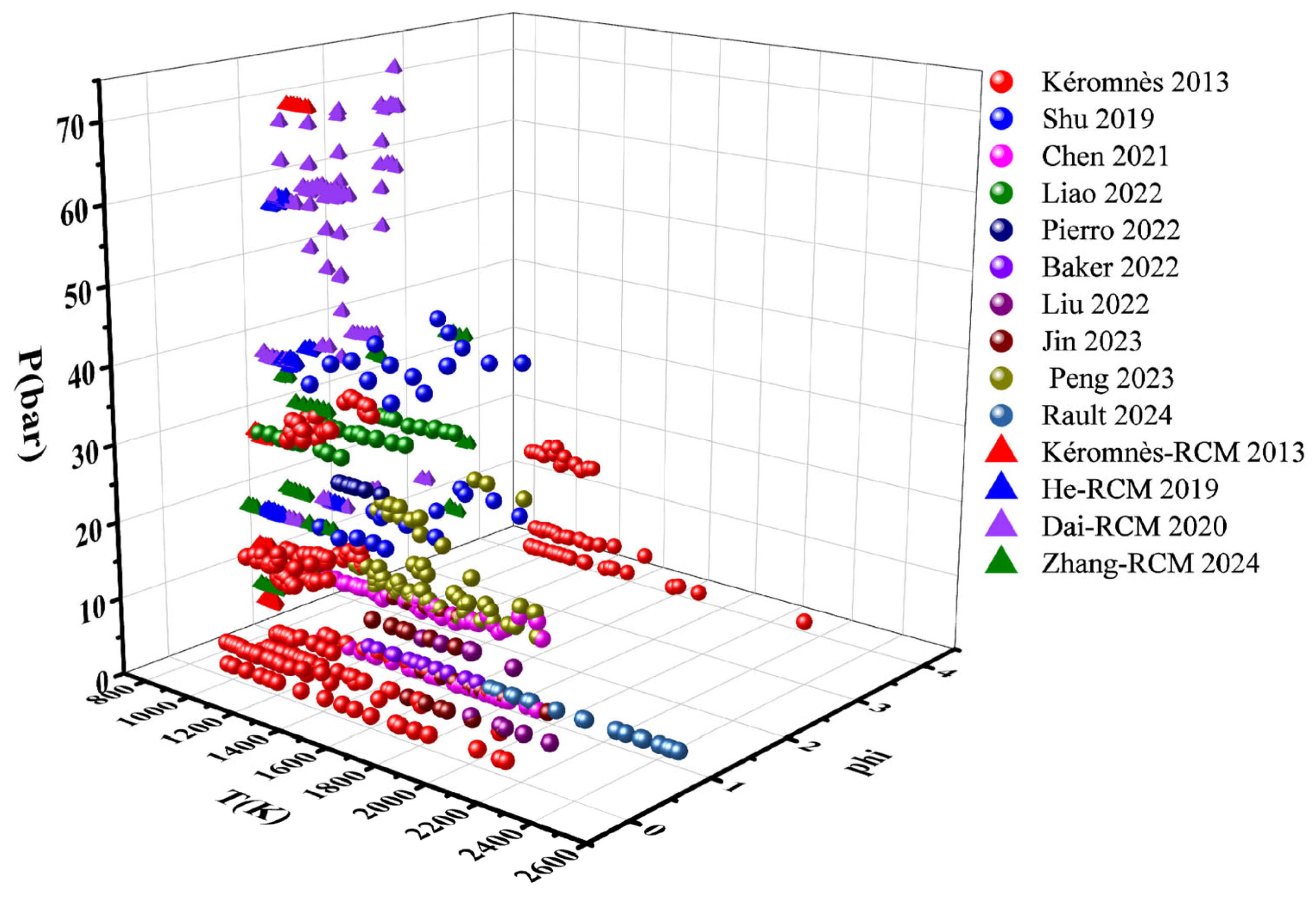
(a) Experiment data: The selection of simulation conditions plays a critical role in determining the accuracy with which the surrogate model represents the chemical process. Experimental conditions were initially gathered from existing studies [10,16,21,23,41,42,43,44,45,46,47,48,49,50]. Simulations were conducted based on these conditions. The distribution of the experimental data is shown in Figure 3. Upon reviewing the data, it was observed that IDT experiments for ammonia–hydrogen combustion cover equivalence ratios of 0.1, 0.3, 0.5, 1.0, and 1.5, with a temperature range of 930 K to 2480 K and pressures ranging from 1 bar to 70 bar. Due to variations in the heat dissipation curves of the rapid compression machines used across different laboratories, IDT experimental data from shock tubes were selected for further analysis. Simulations were performed using Cantera. A total of 364 experimental data points were used, covering hydrogen mole fractions of 0%, 5%, 30%, 50%, and 100%, equivalence ratios of 0.1, 0.3, 0.5, 1.0, 2.0, and 4.0, and a temperature range of 935 K to 2285 K. Additionally, the LFS experimental data [51] were employed as test data for the mechanism, spanning hydrogen fuel mole fractions of 0%, 5%, 10%, 20%, 30%, 40%, 50%, and 60%, equivalence ratios of 0.8, 0.9, 1.0, 1.1, 1.2, 1.3, and 1.4, and temperatures ranging from 298 K to 473 K, including specific temperatures of 298 K, 323 K, 373 K, 423 K, and 473 K.

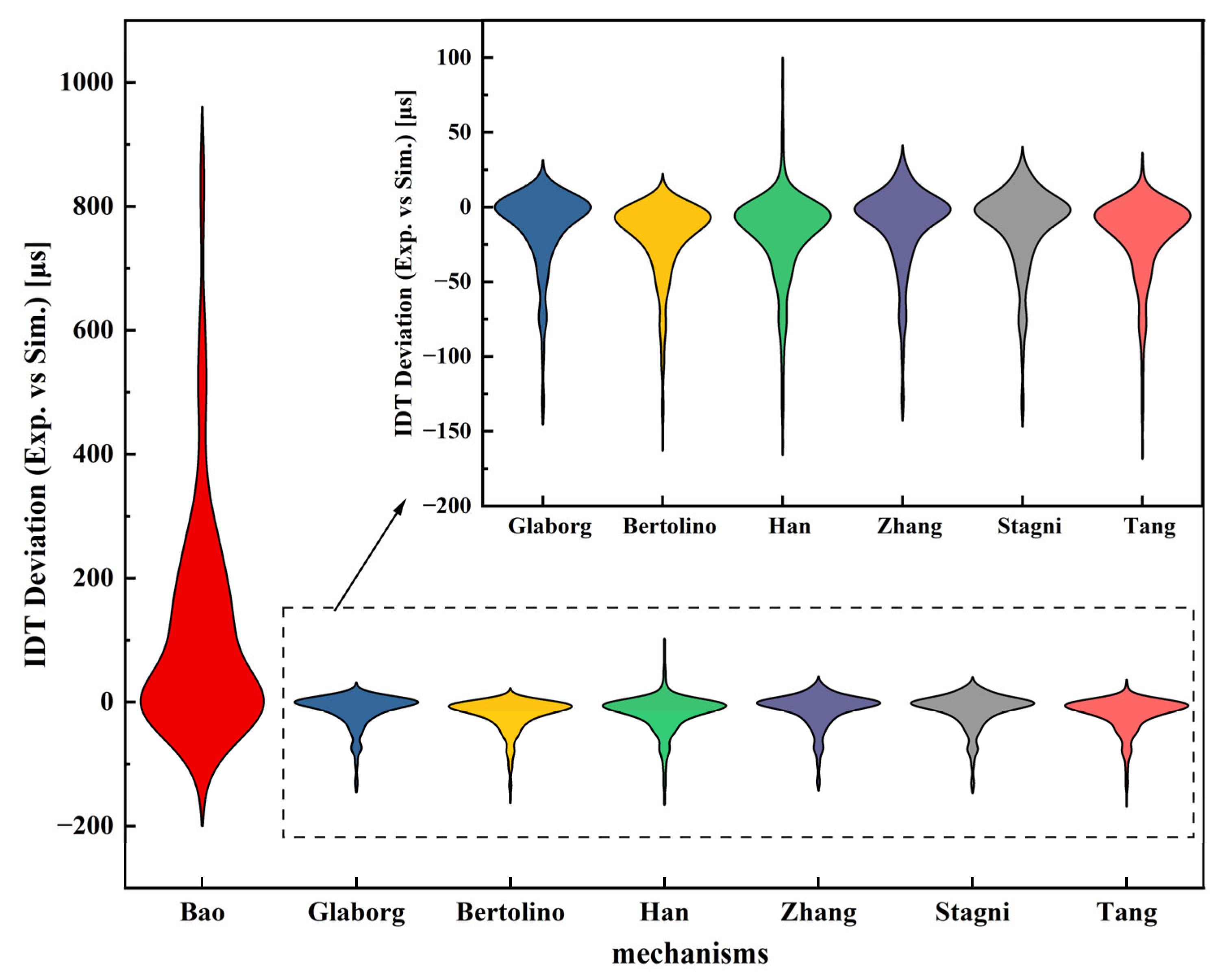
(b) basic mechanism: The latest ammonia–hydrogen combustion mechanisms include research by Bertolino 2021 [52], Han 2021 [53], Bao 2022 [54], Tang 2022 [55], Glaborg 2023 [56], Stagni 2023 [57], and Zhang 2024 [58]. Figure 4 illustrates the performance of these mechanisms compared with collected experimental data. The y-axis represents the deviation between the simulation results and experimental values, while the x-axis corresponds to the mechanisms from different sources in the literature. The violin plot demonstrates the distribution of deviations for each mechanism. The Bao mechanism exhibits a larger deviation, with a range exceeding 200 microseconds, indicating a substantial mismatch between the Bao mechanism and the experimental data. In the zoomed-in plot, the extended upper tail of the Han mechanism suggests the presence of more extreme values. Based on the overall distribution of deviations and the number of reactions in each mechanism, the Stagni mechanism, which includes 31 species and 205 reactions, was ultimately selected.

(c) Sensitivity analysis: Among these 205 reactions, sensitivity analysis was performed to identify the 20 most influential reactions for optimization. To ensure the accuracy of the mechanism under engine operating conditions, typical conditions were selected for the analysis: 100% NH₃, p = 20 bar, ϕ = 0.5, 1200 K/1000 K; 70% NH₃, p = 10 bar, ϕ = 1, 1200 K/1000 K. These analyses were conducted using CHEMKIN. Figure 5 and Figure 6 illustrate the sensitivity reactions under these different conditions: panel (a) shows reactions sensitive to both temperatures, while panels (b) and (c) highlight reactions unique to 1000 K and 1200 K, respectively. To identify reactions that are sensitive across the conditions, a heatmap is presented in Figure 7. The 20 most sensitive reactions were selected and listed in

Table 2. Highly sensitive reactions of IDT. These parameters are quantified using the Arrhenius equation k =AT^βexp[-E/(RT)], with units specified as cm³, mol, K and cal.

Reaction Number	Reaction	A	$\mathsf{\beta }$	E	UF	Ref.
5	O2 + H <=> O + OH	1.14 × 1014	0	1.5286 × 104	1.2	[59]
22	H + O2 (+M) <=> HO2 (+M)(high-P-rate-constant)	4.65 × 1012	0.44	0.0	1.2	[60]
29	NH3 + HO2 <=> NH2 + H2O2	1.173	3.839	1.726 × 104	2	[61]
36	NH2 + O2 <=> H2NO + O	2.6 × 1011	0.487	2.905 × 104	1.5	[62]
37	NH2 + HO2 <=> H2NO + OH	1.02 × 1012	0.166	−938.0	2	[63]
39	NH2 + HO2 <=> NH3 + O2	5.91 × 107	1.59	−1373.0	2	[63]
40	NH2 + HO2 <=> HNO + H2O	2.19 × 109	0.791	−1428.0	2	[63]
46	NH2 + NH2 <=> NH3 + NH	5.64	3.53	550.0	1.5	[64]
47	NH2 + NH2 <=> N2H4 (p=10 atm)	3.2 × 1049	−11.18	1.39885 × 104	1.2	[63]
76	NH2 + NO2 <=> H2NO + NO	8.6 × 1011	0.11	−1186.0	2	[65]
77	NH2 + NO2 <=> N2O + H2O	2.2 × 1011	0.11	−1186.0	1.5	[66]
78	NH2 + NO <=> N2 + H2O	2.6 × 1019	−2.369	870.0	1.5	[66,67]
79	NH2 + NO <=> NNH + OH	4.3 × 1010	0.294	−866.0	1.5	[66,67]
99	N2H4 + NH2 <=> N2H3 + NH3	3,700,000	1.94	1630	2	[67]
113	N2H2 <=> NNH + H (p=10 atm)	3.1 × 1041	−8.42	7.60042 × 104	2	[67]
142	NO + HO2 <=> NO2 + OH	2.11 × 1012	0	−480	1.5	[68]
163	HONO + NH2 <=> NH3 + NO2	317	2.83	−3570	1.5	[63]
173	H2NO + NH2 <=> HNO + NH3	9.48 × 1012	−0.081	−1643.4	2	[69]
174	H2NO + O2 <=> HNO + HO2	172,300	2.188	1.801 × 104	2	[65]
183	H + NO2 <=> OH + NO	8.85 × 1013	0	0	2	[63]

, along with their parameters from the Stagni mechanism [57].

(d) Perturbation mechanisms for MLP training: Reactions 5 and 22 are part of the hydrogen combustion mechanisms, which have been widely studied and are well-established [62,63], therefore do not require major modifications. Similarly, reaction 47 is well-studied within the ammonia pyrolysis mechanism [63]. When perturbing the parameters of these 20 reactions, several factors were considered, especially due to the presence of multiple parameters for certain reactions. The following strategies were implemented: (1) For reactions with both low-P-rate-constant and high-P-rate-constant, only the parameters of the high-P-rate-constant were modified. The high-P-rate-constant is typically more influential in governing the reaction rate at high pressures, which are common conditions in ammonia–hydrogen engines [58]. (2) For duplicate reactions, where the rate is the sum of individual rates (i.e., k = k₁ + k₂), only one reaction was selected for modification. Despite modifying just one reaction, the rule of summing the rate constants for the combined reaction is still maintained, ensuring that the total rate is correctly described. (3) For plog-type pressure-dependent reactions, only the parameters under high-pressure conditions were modified. The uncertainty of these reactions, listed in the 6th column of Table 2, was determined from the literature. The 64 mechanisms were generated by uniformly sampling the 20 reaction parameters within their uncertainty ranges, with each mechanism representing a different combination of these parameters. The differences between the mechanisms arise from the variations in reaction rates and kinetic behaviors caused by the random combinations of these sampled values. This number is not fixed but is deemed sufficient to cover the possible parameter space.

Figure 7 illustrates the differences between the simulation results and experimental values for the 64 mechanisms across 364 experimental conditions. The x-axis represents the 64 mechanisms, while the y-axis displays the standardized deviation, quantifying the difference between the simulated and experimental values. A small subset of mechanisms (e.g., mech_10) exhibit larger standardized deviations, indicating significant fluctuations in their simulation results. Some mechanisms (e.g., mech_1 and mech_58) have more outliers, implying that their simulations deviate from the experimental results under certain conditions. Based on the above analysis, it can be concluded that the 64 perturbed mechanisms sufficiently encompass the parameters’ space.

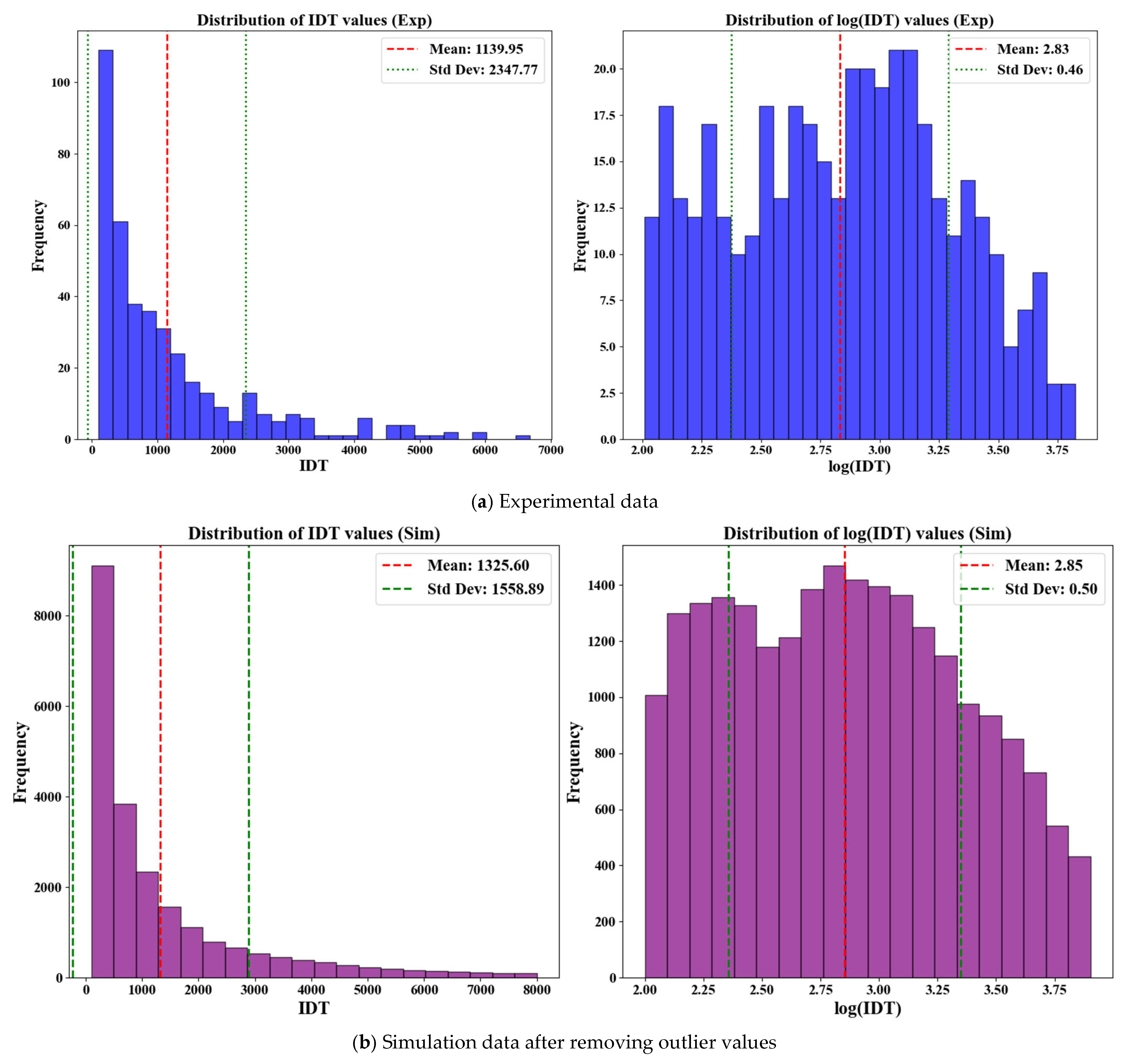
Simulations were conducted on these 64 mechanisms using Cantera. The overall distribution of these simulation results was observed and compared with the distribution of all collected experimental data. Due to variations across these 64 mechanisms, certain simulation results were deemed unrealistic. After analyzing the distribution of experimental data, simulation IDTs exceeding 8000 μs or below 100 μs were excluded. The adjusted distribution of simulation data was found to align more closely with the experimental data, as shown in Figure 8.

2.2. Machine Learning Methods

2.2.1. Comparative Methods

Generalized linear regression (GLR) is an extended form of traditional linear regression. Its core lies in using linear functions combined with link functions to describe the relationships between variables [70]. For parameter estimation, GLR mostly adopts the maximum likelihood estimation method, enabling more efficient utilization of data information. Support vector machines (SVMs) are a class of flexible supervised learning models. Their core objective is to find the optimal hyperplane in the feature space to achieve data classification or regression [71]. Random Forest (RF) is an algorithm based on the concept of “ensemble learning”. It generates multiple decision trees through random sampling, and then integrates the results of individual decision trees by means of voting (for classification tasks) or averaging (for regression tasks) [72].

2.2.2. Surrogate Model

The surrogate model incorporates a DNN that is trained to map the relationship between initial conditions, mechanism parameters, and simulated IDT. This model is then used to optimize mechanism parameters by mapping initial conditions to experimental IDT. By computing the loss function between the experimental and predicted results, the optimized mechanism file is produced.

(a) DNN: DNN is used to model the relationship between initial conditions, reaction parameters, and IDT. This study compares three NN architectures: MLP, LeNet-5, and ResNet. They all use the SiLU [73] activation function. The MLP represents a class of neural networks that effectively learns complex, nonlinear relationships between inputs and outputs [74]. LeNet-5 [75] is one of the earliest convolutional neural network (CNN) models, originally developed for handwritten character recognition. It comprises 7 layers in total, encompassing 2 convolutional layers, 2 pooling layers, and 3 fully connected layers. ResNet-18 [76] is designed to tackle gradients vanishing and gradient exploding issues during the training of DNNs. Its key concept involves introducing residual blocks, enabling the network to more effectively train deeper structures. The training output of the ResNet model is expressed as follows:

$$X_{i+1}=F\left(X_i\right)+X_i$$

(1)

where $X_{i+1}$ refers to the output of the residual block, while $X_i$ represents the input of the residual block.

The input to DNN consists of 623 variables, including 8 initial conditions and 615 reaction parameters. The outputs are the logarithmic values of IDT. The dataset was divided into training, validation, and test sets in an 8:1:1 ratio.

It should be noted that the training data used here are simulation data, generated using Cantera. The final dataset contains 22,607 IDT values, with 18,017 in the training set, 2092 in the validation set, and 2498 in the test set.

(b) Surrogate model: Figure 9 shows the workflow of the surrogate model. The surrogate model receives 8 initial conditions as input, with the first layer consisting of a tensor of dimension 615, which incorporates all parameters for 205 reactions. For each reaction, a corresponding mask is assigned to determine whether the parameters should be optimized. The mask is created based on information in the mechanism file, specifically by using a flag labeled ‘modify_param’ within the YAML file. In the YAML file, each reaction is associated with the ‘modify_param’ field, which is set to true or false. When the ‘modify_param’ value is true, the corresponding mask value is set to 1, indicating that the parameters for that reaction need to be optimized. Conversely, when ‘modify_param’ is false, the mask is set to 0, meaning the parameters are not optimized. This allows selective optimization of reaction parameters based on predefined conditions in the mechanism file. During model training, the surrogate model checks the ‘modify_param’ values for each reaction and assigns the appropriate mask value accordingly. Following the first layer, the inputs are concatenated with the 8 initial conditions and 615 parameters, producing a 623-dimensional vector. This vector is then passed through the DNN model, whose parameters are loaded from the pre-trained state and set to be non-trainable. This ensures that the parameters remain unchanged during this step. During the optimization process, the network parameters of the DNN model remain fixed, and backpropagation only optimizes the marked parameters in the first layer. This setup ensures that the DNN accurately maps the simulation process, while the surrogate model solely focuses on optimizing the mechanism parameters.

The loss is computed by comparing the experimental data with the outputs. During the loss backward propagation, we employ PyTorch (v2.2.2)’s automatic differentiation—a reverse-mode implementation consistent with standard backpropagation—to compute gradients, enabling efficient model optimization. Parameter updates in the surrogate model are based on the principle of gradient descent, where the gradients are computed and used to adjust the first layer’s parameters. This process is stopped when the validation loss does not improve for a set number of epochs, defined by a patience parameter. In this study, a patience value of 20 was used, meaning that if there was no improvement in the validation loss for 20 consecutive epochs, the training would be halted, helping to prevent overfitting and unnecessary computation. It is crucial to note that the parameters in the first layer are not only network parameters but also reaction parameters. Therefore, the upper and lower bounds for these parameters are determined based on the uncertainty of the corresponding reactions and are incorporated into the design of the loss function to ensure that the physical relevance of the parameters is maintained throughout the optimization process. The design of the loss function is as follows:

Equation (2) represents the inverse normalization of the parameters in the first layer,

$$p_{original}=p_{tensor}\cdot {\sigma }_{\ln A}+{\mu }_{\ln A}$$

(2)

where $p_{tensor}$ refers to the parameters that were previously normalized before being input into the network, while ${\sigma }_{\ln A}$ and ${\mu }_{\ln A}$ represent the standard deviation and mean of the $\ln A$, respectively.

Equation (3) introduces a normal distribution constraint to the inversely normalized parameters,

$${\mathrm{L}}_{\mathrm{r}\mathrm{e}\mathrm{g}}=\lambda \cdot \sum _{j=1}^M{\left(p_{origial,j}-{\mu }_j\right)}^2/{\sigma }_j^2$$

(3)

where $p_{origial,j}$ refers to the original (inversely normalized) parameter value for the j-th parameter, ${\mu }_j$ is the mean of the normal distribution for the$j$-th parameter, derived from empirical data and ${\sigma }_j$ is the standard deviation for the $j$-th parameter, also derived from empirical data. In this paper, ${\mu }_j$ and ${\sigma }_j$ values from the original mechanism are used to limit the optimization space for the parameters. $\lambda$ is a hyperparameter that controls the strength of the regularization.

Equation (4) represents the Mean Squared Error (MSE) loss for IDT,

$${\mathrm{L}}_{\mathrm{I}\mathrm{D}\mathrm{T}}=\sum _{i=1}^M{\left(y_i-\widehat{y_i}\right)}^2$$

(4)

where $y_i$ refers to the actual IDT value. $\widehat{y_i}$ is the predicted IDT.

Equation (5) represents the total loss function used in the model, combining the MSE loss for IDT and the regularization loss.

$$\mathrm{L}={\mathrm{L}}_{\mathrm{I}\mathrm{D}\mathrm{T}}+{\mathrm{L}}_{\mathrm{r}\mathrm{e}\mathrm{g}}$$

(5)

2.3. Evaluation of Models

The predictive performance of the test set was assessed using two indicators: R² and RMSE. The formula for R² is given by Equation (6).

$${\mathrm{R}}^2={\displaystyle \frac{\sum _{j=1}^n{\left(y_j-\widehat{y_j}\right)}^2}{\sum _{j=1}^n{\left(y_j-\overline{y_j}\right)}^2}}$$

(6)

Here, $y_j$ stands for the experimental IDT, $\widehat{y_j}$ denotes the predicted IDT, and $\overline{y_j}$ represents the mean of predicted IDT values. R² ranges from 0 to 1: a value of 0 indicates no correlation between the experimental and predicted IDT values, while a value close to 1 signifies a strong positive linear relationship between them, meaning the regression model fully accounts for the variation in predicted IDT values. The second indicator is RMSE, whose mathematical formulation is provided in Equation (7).

$$\mathrm{RMSE}=\sqrt{{\displaystyle \frac{1}{n}}{\sum }_{j=1}^n{\left(y_j-\widehat{y_j}\right)}^2}$$

(7)

3. Results

3.1. Surrogate Model Optimization

3.1.1. The Predictive Capability of Neurons Within the Hidden Layers of MLP

The count of hidden layers, a key parameter, influences the network’s predictive performance and governs computational time. The learning rate was configured to 0.0001. Figure 10 illustrates the optimization of hidden layers by adjusting their number from two to ten in steps of one, with all other hyperparameters kept constant. Notably, the maximum R² value of 0.9858 was achieved when using seven layers. As the layer count increased, the R² value showed little fluctuation, and the RMSE value was 184. However, further increasing the depth to 10 layers does not yield additional gains. On the contrary, it results in signs of overfitting, as indicated by the increased validation loss. These results suggest that the seven-layer architecture is sufficiently expressive for modeling the problem without introducing unnecessary complexity.

Moreover, the number of epochs required to reach the optimum network performance is optimized by adjusting the epoch count from 300 to 2000, with the remaining hyperparameters held constant. As shown in Figure 11, calculations were performed for epochs of 300, 500, 1000, 1200, 1500, 1800, and 2000. At 300 epochs, the R² was 0.4945 and the RMSE was 1099, with the network not converging at this point. When the number of epochs reached 1500, the maximum R² of 0.9807 and the minimum RMSE of 239 were recorded. When the number of epochs was further increased from 1500, there was almost no improvement in network optimization.

3.1.2. Optimization of DNN

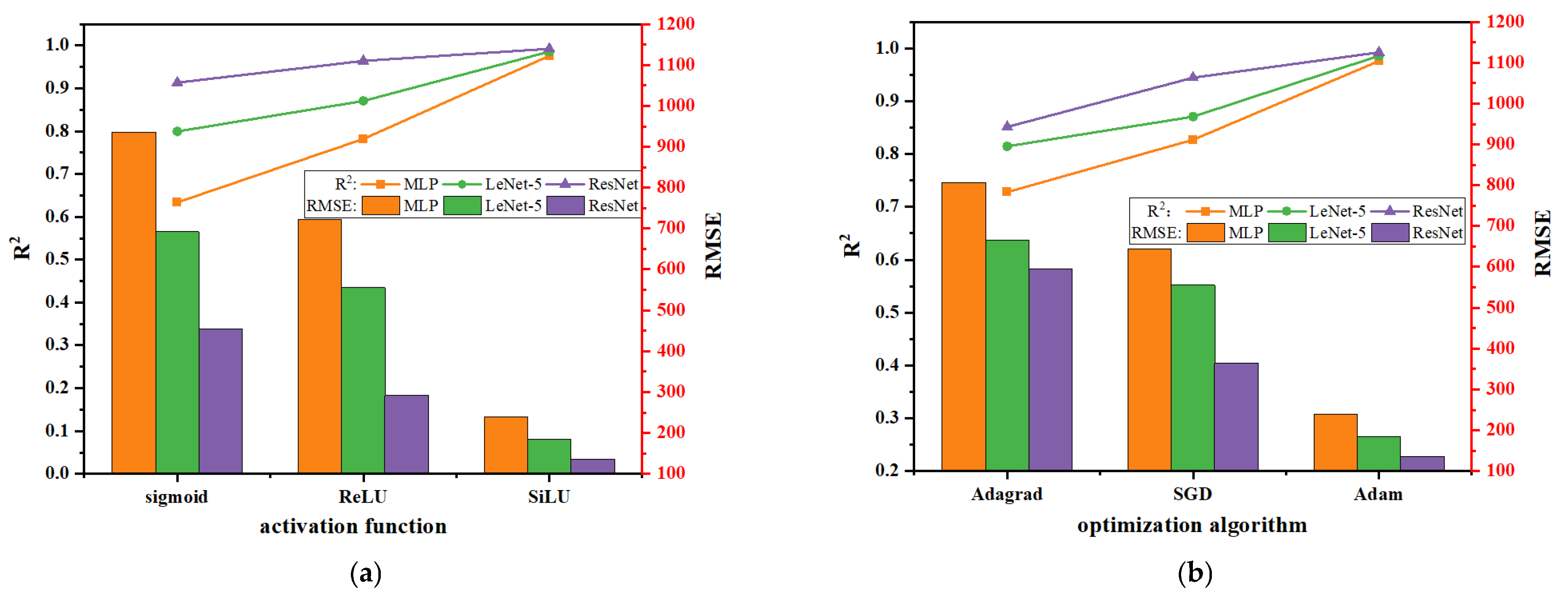
Figure 12a illustrates the tuning of activation functions within neural networks, comparing the previously optimized seven-layer MLP with LeNet-5 and ResNet. As shown in the figure, for the MLP, LeNet-5, and ResNet, the activation function of the Sigmoid type exhibits the lowest R² values (0.6337, 0.79942, 0.91346) and the highest RMSE values (935, 692, 454), respectively. Nevertheless, among all tested activation functions, the SiLU activation function exhibited superior performance metrics, with R² of 0.9807, 0.9858, and 0.9923, and RMSE of 239, 184, and 136 for the MLP, LeNet-5, and ResNet, respectively. Due to the randomization weights and biases of neuron, the predictive results across different prediction methods can vary slightly. When the SiLU activation function is adopted within the network, the prediction values have reached close to the actual values.

Figure 12b depicts the tuning of different optimization functions, including Adagrad, stochastic gradient descent (SGD), and Adam. The network was optimized via these three functions, with all other hyperparameters held constant. It is concluded that Adam delivered superior performance with the lowest RMSE of 239, 184, and 136 for the MLP, LeNet-5, and ResNet, respectively. Therefore, the SiLU activation function and Adam optimization function will be used for subsequent calculations.

3.1.3. Comparison Among Diverse Machine Learning Models

Of the machine learning approaches employed in this study, GLR exhibited the lowest predictive accuracy, with a notable discrepancy between the predicted values and actual values of the test set. From Figure 13a, GLR predicted IDTs that are notably overestimated for values below 2000 μs, and underpredicted above this value. From Figure 13b, SVM notably outperformed GLR in terms of predictive performance. From Figure 13c, RF exhibited high predictive accuracy for low IDT values under 3000 μs. For the prediction accuracy of the three DNNs: MLP had an R² value of 0.9807; the prediction accuracy of LeNet-5 was further improved, with an R² value of 0.9858; and a predictive performance approaching 99% was reached for the ResNet, which could satisfactorily predict the experimental data values at both low and high IDT magnitudes, as shown in Figure 13d–f.

Table 3. Comparison among diverse machine learning approaches.

Models	R2	RMSE
GLR	0.5855	995
SVM	0.8971	496
RF	0.9761	239
MLP	0.9807	214
LeNet-5	0.9858	184
ResNet	0.9923	135

provides a detailed comparison complete with corresponding values. Neural Networks are generally more suitable for nonlinear problems, given their ability to model the complex relationships between input features and outputs with greater effectiveness. Figure 14 presents the prediction results, 95% confidence intervals, and precision evaluation of the ResNet model on the test set for IDT. Among them, the blue scatter points represent the samples in the test set; the red curve is the fitted curve between the predicted values and the experimental values; the green 95% Confidence Band and the pink 95% Prediction Band are both constructed based on approximately 2 times the standard deviation, quantifying the uncertainty intervals for model parameter estimation and new sample prediction, respectively. It should be noted that the neural network in this study is trained based on the logarithmic values of IDT. Although the coefficient of determination R² has reached 0.9923, due to the inverse process of logarithmic transformation amplifying the fluctuations in the original value range, there are still a small number of data points outside the 95% Prediction Band at the original IDT scale.

3.1.4. Optimization in Surrogate Model

The surrogate model was developed based on the trained ResNet. During training, the parameters of the trained ResNet were kept frozen, enabling the surrogate model to concentrate exclusively on optimizing the reaction parameters while leveraging the representational capacity already learned by the trained ResNet. To better explore the optimization landscape, different sets of perturbed reaction parameters were randomly sampled within uncertainty bounds and used as distinct initialization values for the trainable parameters of the surrogate model. Firstly, a small perturbation space comprising 64 mechanisms was generated. The initial MSE loss of the original mechanism was 0.004949. Figure 15 illustrates the MSE loss values before and after optimization for the 64 perturbed mechanisms using the surrogate model. As shown, the optimization process led to a significant reduction in loss by approximately one order of magnitude, from around 0.04 to 0.0028. While this demonstrates improvement, the gains remained limited, likely due to the initial perturbation space being confined to a local minimum region. The perturbation space was expanded to 640 perturbed mechanisms. Figure 16a presents the distribution of the initial loss for these 640 mechanisms using the surrogate model. Considering the inherent approximation error in the surrogate model, a threshold of 0.015 was established to filter out poorly performing mechanisms. As a result, 246 mechanisms with initial loss below this threshold were selected for further optimization. Figure 16b shows that most of these optimized mechanisms achieved loss values converging around 0.0020. The mechanism with the lowest final loss was selected as the optimized mechanism for subsequent analysis.

3.2. Comparison of Different Mechanisms Performance

3.2.1. Validation on IDTs

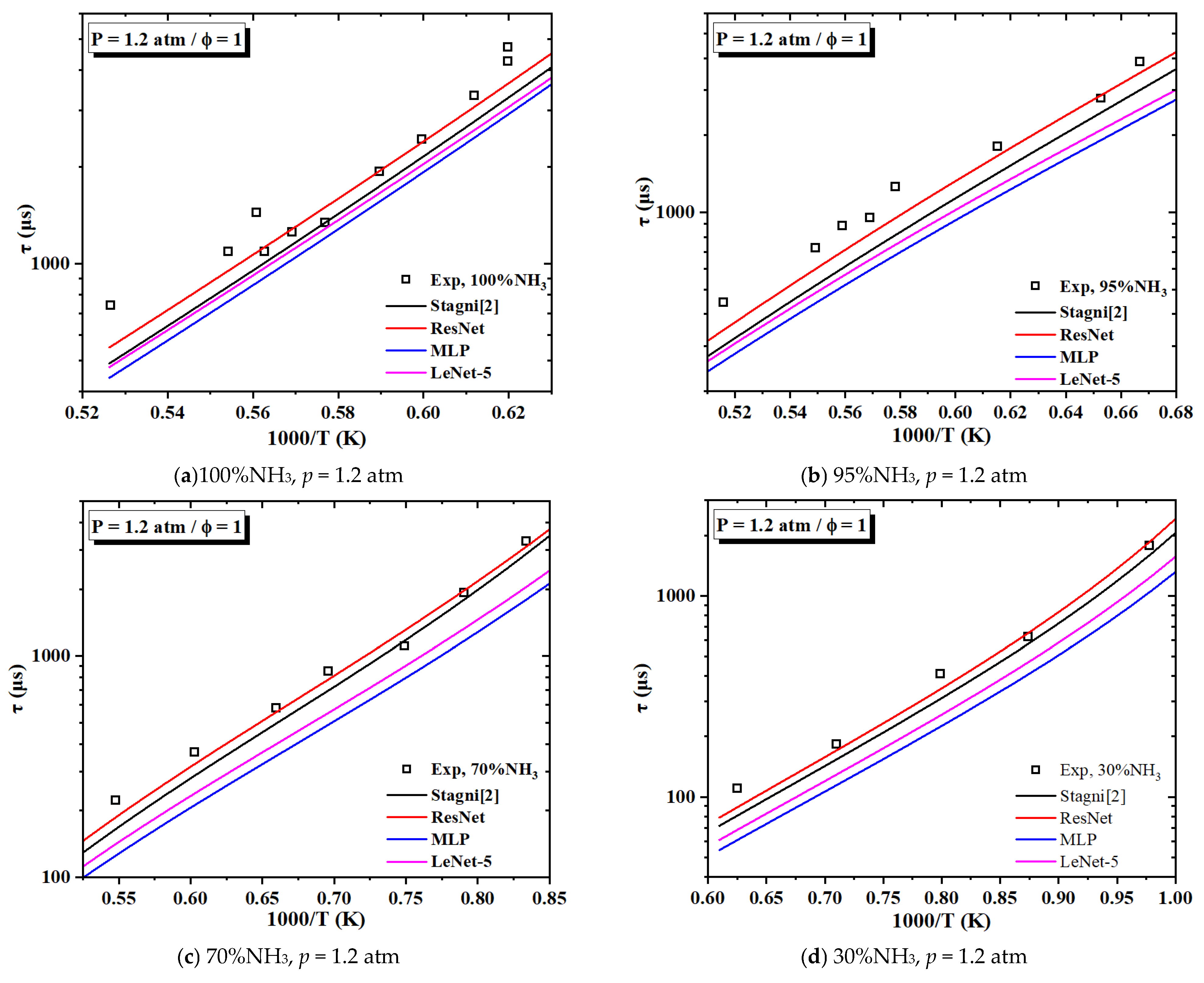
Figure 17 further compares the experimental IDT data from the study by Chen et al. [35] with the simulation results. The mech_ResNet generally shows better fitting performance across varying ammonia fractions and pressures. At high ammonia fractions (e.g., 70% NH₃) and low fractions (e.g., 30% NH₃), the simulation curves from mech_ResNet most effectively capture the variations in IDT. Mech_ResNet demonstrates better predictive performance under both pressure conditions, and its performance is significantly improved under high pressure conditions, making it more suitable for predicting IDTs across different ammonia concentrations. The residual connection structure of ResNet enables it to effectively learn the complex nonlinear relationships between IDT and temperature, ammonia fraction, and pressure. For instance, under different ammonia mole fractions (e.g., 70% NH₃ and 30% NH₃), the variation pattern of IDT exhibits high nonlinearity due to changes in the dominance of key reactions. ResNet’s deep feature extraction capability can capture these subtle changes, whereas the MLP (a simple fully connected network) lacks the ability to model such complex nonlinearities.

The performance improvement of mech_ResNet is particularly significant under high pressure (10 atm). In high-pressure environments, combustion kinetics become more complex, and ResNet’s deep architecture can learn these complex interactions from data more accurately. In contrast, MLP and LeNet-5 exhibit larger prediction errors, as they struggle to model the high-dimensional nonlinearities under high pressure. Traditional machine learning models are often limited by insufficient expressive capacity in scenarios involving complex combustion kinetics, and ResNet’s residual structure precisely addresses this shortcoming. The excellent performance of mech_ResNet under different ammonia volume fractions and pressures stems from the balance between deep feature learning capability (enabled by its residual connections) and data-driven adaptability.

3.2.2. Validation on LFS

Experiment data was obtained from the study by Lhuillier et al. [22]. Figure 18 presents a comparative analysis of the MSE for predicting LFS, evaluating the performance of the original and three different optimized mechanisms. The original mechanism exhibits an MSE of 15.45, serving as a baseline for comparison. While optimizing different numbers of reactions lead to effective decreases in the MSE to 14.65, 14.11, and the lowest value for mech_ResNet, the key aspect might lie in the surrogate model’s generalization ability. Mech_ResNet offers an advantage in predicting LFS, with potentially higher precision and smaller prediction deviations. The improvement of mech_ResNet over the original mechanism is approximately 36.6%, indicating a noticeable reduction in prediction deviation. This reduction in MSE indicates that the optimization approach may effectively capture some of the underlying physical and chemical interactions governing the combustion process. The surrogate model processes IDTs during training to inform the optimization of the reaction mechanism. The optimized mechanism demonstrates enhanced generalization when applied to predict LFS. This showcases the robustness and reliability of the proposed optimization method in improving the predictive accuracy of reaction mechanisms.

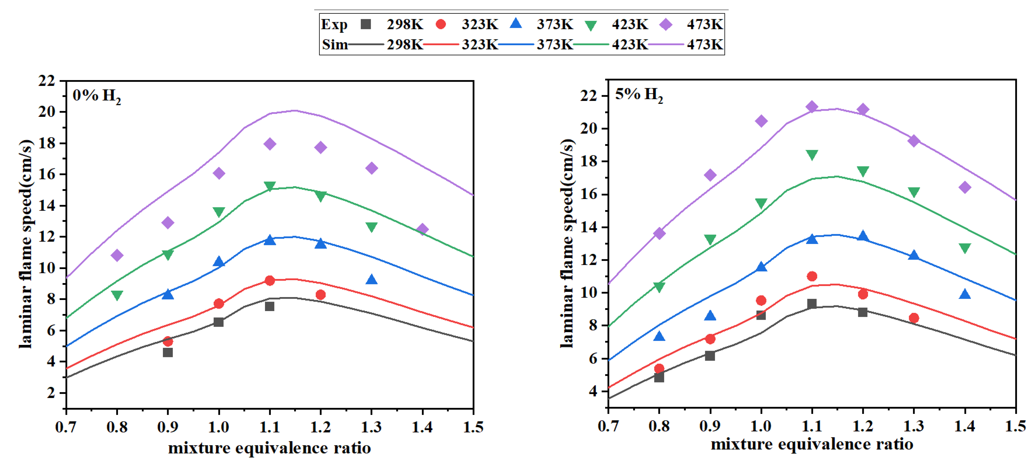
Figure 19 compares the simulation results with experimental data [22] for LFS. Overall, the mech_ResNet provides a better fit to the experimental data under most conditions. Specifically, at different hydrogen mole fractions (0%, 60%), the simulating results show a closer alignment with the experimental data, with the simulation curves exhibiting smoother behavior and more accurately capturing the trend of flame speed variation with equivalence ratio. In conclusion, the mech_ResNet offer improved accuracy in predicting LFS, especially under conditions of high-temperature and varying hydrogen concentrations. This indirectly demonstrates that using a surrogate model to optimize parameters is effective.

3.2.3. Validation of Species Mole Fractions

Validations of the species mole fractions using the optimized mechanism were performed using the experimental results from steady-state oxidations in a jet-stirred reactor (JSR). Figure 20 contrasts the species mole fractions as measured by Zhang et al. [77] in JSR oxidation experiments against simulations employing the optimized mechanism. Specifically, the temperature is varied from 800 K to 1300 K, while the hydrogen fraction in the reactant mixture spans from 0% to 70%. The results show that the optimized mech_RsNet demonstrates remarkable predictive performance. It can accurately predict the evolutions of key species, including NH₃, H₂O, and NO, under different temperature and hydrogen fraction conditions. In the case of NH₃, the predicted mole fraction profiles closely match the experimental data throughout the entire temperature and hydrogen fraction range. Similarly, for H₂O and NO, the optimized mechanism shows excellent agreement with the experimental measurements, suggesting its effectiveness in capturing the complex chemical reactions associated with the JSR oxidation process.

To summarize, the optimized mechanism has shown remarkable accuracy in predicting key macroscopic combustion characteristics of ammonia–hydrogen fuels, including IDTs and LFS. Equally importantly, it demonstrates strong capabilities in capturing microscopic species mole fractions, providing a more comprehensive understanding of the combustion process. The effectiveness of the optimized mechanism is evidenced by its consistent performance under a broad range of conditions, including varying dilution ratios, pressures, hydrogen fractions, temperatures and mixture equivalence ratios. These extensive validations not only affirm the reliability of the optimized mechanism but also suggest that the proposed method can effectively capture the underlying physical and chemical interactions governing the combustion process. This indicates the method has great potential to be a valuable approach for optimizing mechanisms, providing a balanced and reliable solution with high practical significance.

4. Conclusions

DNN was used to construct an IDT simulation model for ammonia–hydrogen air–fuel mixtures, which was then compared to other machine learning techniques. The operating pressure, unburnt temperature, equivalence ratio, and the mole fractions of five species served as the model’s input parameters, while the simulated IDT functioned as its output. Then a surrogate model was based on the trained DNN to optimize mechanism parameters. The main conclusions are as follows:

• MLP performed better with seven layers and 1500 epochs. Following the optimization of its activation function and optimization algorithms on the test set—comprising the IDTs of ammonia–hydrogen under varying operating pressures, temperatures, and equivalence ratios—the MLP model delivered improved performance with an R² of 0.9807 and RMSE of 239.
• LeNet-5 and ResNet markedly enhanced the prediction accuracy of the DNN model, thereby achieving an R² of 0.9858, and 0.9923 and RMSE of 184, and 136, respectively. ResNet was used as a part of the surrogate model to further optimize the mechanism parameters.
• The optimized mechanism outperforms the original mechanism when tested with experimental data. For IDT simulations, mech_ResNet exhibits smaller deviations. For LFS simulations, mech_ResNet improves the prediction accuracy by approximately 36.6% compared to the original mechanism.

In subsequent research, a thorough investigation of DNN models aimed at optimizing all parameters in the mechanism will serve as the primary focus.

References

1. Erfani, N.; Baharudin, L.; Watson, M. Recent Advances and Intensifications in Haber-Bosch Ammonia Synthesis Process. Chem. Eng. Process.-Process Intensif. 2024, 204, 109962. [Google Scholar] [CrossRef]
2. Xin, T.; Li, S.; Yang, W.; Li, X.; Li, R.; Xu, C. Thermodynamic Comparison of Cryogenic Air Separation Units with External and Internal Compression of Oxygen Designed for the Coal-Fueled Allam Cycle. Energy 2025, 333, 137325. [Google Scholar] [CrossRef]
3. Ashida, Y.; Arashiba, K.; Nakajima, K.; Nishibayashi, Y. Molybdenum-Catalysed Ammonia Production with Samarium Diiodide and Alcohols or Water. Nature 2019, 568, 536–540. [Google Scholar] [CrossRef] [PubMed]
4. Yandulov, D.V.; Schrock, R.R. Catalytic Reduction of Dinitrogen to Ammonia at a Single Molybdenum Center. Science 2003, 301, 76–78. [Google Scholar] [CrossRef] [PubMed]
5. Mohamed, A.M.O.; Economou, I.G.; Bicer, Y. Navigating Ammonia Production Routes: Life Cycle Assessment Insights for a Sustainable Future. Curr. Opin. Green Sustain. Chem. 2024, 49, 100947. [Google Scholar] [CrossRef]
6. Xu, X.; Wang, W.; Qi, Y.; Wang, Z.; Min, H.; Li, F.; Yin, Y.; Li, Z. Numerical Simulation of Ammonia-Hydrogen Engine Using Low-Pressure Direct Injection (LP-DI); No. 2024–1–2118; SAE International: Detroit, MI, USA, 2024. [Google Scholar]
7. Li, J.; Huang, H.; Kobayashi, N.; He, Z.; Nagai, Y. Study on Using Hydrogen and Ammonia as Fuels: Combustion Characteristics and NO xFormation: Hydrogen and Ammonia as Fuels. Int. J. Energy Res. 2014, 38, 1214–1223. [Google Scholar] [CrossRef]
8. Xiao, H.; Valera-Medina, A.; Bowen, P.J. Modeling Combustion of Ammonia/Hydrogen Fuel Blends under Gas Turbine Conditions. Energy Fuels 2017, 31, 8631–8642. [Google Scholar] [CrossRef]
9. Xiao, H.; Howard, M.; Valera-Medina, A.; Dooley, S.; Bowen, P.J. Study on Reduced Chemical Mechanisms of Ammonia/Methane Combustion under Gas Turbine Conditions. Energy Fuels 2016, 30, 8701–8710. [Google Scholar] [CrossRef]
10. Liu, S.; Zou, C.; Song, Y.; Cheng, S.; Lin, Q. Experimental and Numerical Study of Laminar Flame Speeds of CH4/NH3 Mixtures under Oxy-Fuel Combustion. Energy 2019, 175, 250–258. [Google Scholar] [CrossRef]
11. Zhang, R.; Zhang, Q.; Qi, Y.; Yang, B.; Wang, Z. Investigation on Flame Propagation and End-Gas Auto-Ignition of Ammonia/Hydrogen in a Full-Field-Visualized Rapid Compression Machine. Proc. Combust. Inst. 2024, 40, 105455. [Google Scholar] [CrossRef]
12. Lin, Z.; Liu, S.; Sun, Q.; Qi, Y.; Wang, Z.; Li, J. Effect of Injection and Ignition Strategy on an Ammonia Direct Injection–Hydrogen Jet Ignition (ADI-HJI) Engine. Energy 2024, 306, 132502. [Google Scholar] [CrossRef]
13. Lin, Z.; Liu, S.; Sun, Q.; Qi, Y.; Wang, Z. Numerical Investigation of Multiple Hydrogen Injection in a Jet Ignition Ammonia-Hydrogen Engine. Int. J. Hydrogen Energy 2024, 77, 336–346. [Google Scholar] [CrossRef]
14. Wang, Z.; Qi, Y.; Sun, Q.; Lin, Z.; Xu, X. Ammonia Combustion Using Hydrogen Jet Ignition (AHJI) in Internal Combustion Engines. Energy 2024, 291, 130407. [Google Scholar] [CrossRef]
15. Miller, J.A.; Smooke, M.D.; Green, R.M.; Kee, R.J. Kinetic Modeling of the Oxidation of Ammonia in Flames. Combust. Sci. Technol. 1983, 34, 149–176. [Google Scholar] [CrossRef]
16. Fenimore, C.P.; Jones, G.W. Oxidation of Ammonia in Flames. J. Phys. Chem. 1961, 65, 298–303. [Google Scholar] [CrossRef]
17. Lyon, R.K.; Hardy, J.E. Discovery and Development of the Thermal DeNOx Process. Ind. Eng. Chem. Fundam. 1986, 25, 19–24. [Google Scholar] [CrossRef]
18. Lindstedt, R.P.; Lockwood, F.C.; Selim, M.A. Detailed Kinetic Modelling of Chemistry and Temperature Effects on Ammonia Oxidation. Combust. Sci. Technol. 1994, 99, 253–276. [Google Scholar] [CrossRef]
19. Lindstedt, R.P.; Lockwood, F.C.; Selim, M.A. A Detailed Kinetic Study of Ammonia Oxidation. Combust. Sci. Technol. 1995, 108, 231–254. [Google Scholar] [CrossRef]
20. Otomo, J.; Koshi, M.; Mitsumori, T.; Iwasaki, H.; Yamada, K. Chemical Kinetic Modeling of Ammonia Oxidation with Improved Reaction Mechanism for Ammonia/Air and Ammonia/Hydrogen/Air Combustion. Int. J. Hydrogen Energy 2018, 43, 3004–3014. [Google Scholar] [CrossRef]
21. Song, Y.; Hashemi, H.; Christensen, J.M.; Zou, C.; Marshall, P.; Glarborg, P. Ammonia Oxidation at High Pressure and Intermediate Temperatures. Fuel 2016, 181, 358–365. [Google Scholar] [CrossRef]
22. Baker, J.B.; Rahman, R.K.; Pierro, M.; Higgs, J.; Urso, J.; Kinney, C.; Vasu, S. Experimental Ignition Delay Time Measurements and Chemical Kinetics Modeling of Hydrogen/Ammonia/Natural Gas Fuels. J. Eng. Gas Turbines Power 2023, 145, 41002. [Google Scholar] [CrossRef]
23. Wang, H.; Xu, R.; Wang, K.; Bowman, C.T.; Hanson, R.K.; Davidson, D.F.; Brezinsky, K.; Egolfopoulos, F.N. A Physics-Based Approach to Modeling Real-Fuel Combustion Chemistry-I. Evidence from Experiments, and Thermodynamic, Chemical Kinetic and Statistical Considerations. Combust. Flame 2018, 193, 502–519. [Google Scholar] [CrossRef]
24. Saggese, C.; Wan, K.; Xu, R.; Tao, Y.; Bowman, C.T.; Park, J.-W.; Lu, T.; Wang, H. A Physics-Based Approach to Modeling Real-Fuel Combustion Chemistry–V. NO Formation from a Typical Jet A. Combust. Flame 2020, 212, 270–278. [Google Scholar] [CrossRef]
25. Tao, Y.; Xu, R.; Wang, K.; Shao, J.; Johnson, S.E.; Movaghar, A.; Han, X.; Park, J.-W.; Lu, T.; Brezinsky, K.; et al. A Physics-Based Approach to Modeling Real-Fuel Combustion Chemistry–III. Reaction Kinetic Model of JP10. Combust. Flame 2018, 198, 466–476. [Google Scholar] [CrossRef]
26. Xu, R.; Wang, K.; Banerjee, S.; Shao, J.; Parise, T.; Zhu, Y.; Wang, S.; Movaghar, A.; Lee, D.J.; Zhao, R.; et al. A Physics-Based Approach to Modeling Real-Fuel Combustion Chemistry–II. Reaction Kinetic Models of Jet and Rocket Fuels. Combust. Flame 2018, 193, 520–537. [Google Scholar] [CrossRef]
27. Wang, K.; Xu, R.; Parise, T.; Shao, J.; Movaghar, A.; Lee, D.J.; Park, J.-W.; Gao, Y.; Lu, T.; Egolfopoulos, F.N.; et al. A Physics-Based Approach to Modeling Real-Fuel Combustion Chemistry–IV. HyChem Modeling of Combustion Kinetics of a Bio-Derived Jet Fuel and Its Blends with a Conventional Jet A. Combust. Flame 2018, 198, 477–489. [Google Scholar] [CrossRef]
28. Buras, Z.J.; Safta, C.; Zádor, J.; Sheps, L. Simulated Production of OH, HO2, CH2O, and CO2 during Dilute Fuel Oxidation Can Predict 1st-Stage Ignition Delays. Combust. Flame 2020, 216, 472–484. [Google Scholar] [CrossRef]
29. Shi, W.; Wang, Z.; Zhang, H.; Zhang, Y.; Zhang, Z.; Zhao, X. The Reduced Mechanism of Ammonia/Hydrogen Mixture for Detonation. Int. J. Hydrogen Energy 2025, 139, 481–495. [Google Scholar] [CrossRef]
30. Yin, G.; Xiao, B.; You, J.; Zhan, H.; Hu, E.; Huang, Z. Experimental and Kinetic Modeling Study on Propane Enhancing the Laminar Flame Speeds of Ammonia. Fuel Process. Technol. 2023, 247, 107779. [Google Scholar] [CrossRef]
31. Xing, Z.; Freitas, R.S.M.; Jiang, X. Neural Network Potential-Based Molecular Investigation of Thermal Decomposition Mechanisms of Ethylene and Ammonia. Energy AI 2024, 18, 100454. [Google Scholar] [CrossRef]
32. Meng, X.; Shen, D.; Zhu, W.; Zhang, M.; Wu, X.; Zhu, W.; Long, W.; Bi, M. A Combustion Mechanism Simplification and Optimization Method Using Two-Stage Deep Neural Networks for Multiple Fuels. Energy 2025, 335, 137943. [Google Scholar] [CrossRef]
33. Zhou, L.; Song, Y.; Ji, W.; Wei, H. Machine Learning for Combustion. Energy AI 2022, 7, 100128. [Google Scholar] [CrossRef]
34. Aliramezani, M.; Koch, C.R.; Shahbakhti, M. Modeling, Diagnostics, Optimization, and Control of Internal Combustion Engines via Modern Machine Learning Techniques: A Review and Future Directions. Prog. Energy Combust. Sci. 2022, 88, 100967. [Google Scholar] [CrossRef]
35. Üstün, C.E.; De Freitas, R.D.S.M.; Okafor, E.C.; Shahbakhti, M.; Jiang, X.; Paykani, A. Machine Learning Applications for Predicting Fuel Ignition and Flame Properties: Current Status and Future Perspectives. Energy Fuels 2025, 39, acs.energyfuels.5c02343. [Google Scholar] [CrossRef]
36. Shahpouri, S.; Norouzi, A.; Hayduk, C.; Fandakov, A.; Rezaei, R.; Koch, C.R.; Shahbakhti, M. Laminar Flame Speed Modeling for Low Carbon Fuels Using Methods of Machine Learning. Fuel 2023, 333, 126187. [Google Scholar] [CrossRef]
37. Yue, W.; Zhang, B.; Zhang, S.; Wang, B.; Xia, Y.; Liang, Z. A Deep Learning Model for Predicting the Laminar Burning Velocity of NH3/H2/Air. Appl. Sci. 2024, 14, 9603. [Google Scholar] [CrossRef]
38. Liu, L.; Tan, F.; Wu, Z.; Wang, Y. Combining Genetic Algorithm and Deep Learning to Optimize a Chemical Kinetic Mechanism of Ammonia under High Pressure. Fuel 2024, 360, 130508. [Google Scholar] [CrossRef]
39. Pulga, L.; Bianchi, G.M.; Falfari, S.; Forte, C. A Machine Learning Methodology for Improving the Accuracy of Laminar Flame Simulations with Reduced Chemical Kinetics Mechanisms. Combust. Flame 2020, 216, 72–81. [Google Scholar] [CrossRef]
40. Kang, J.; Im, S. Development of a Global Mechanism for Ammonia Combustion Assisted by Machine Learning. J. Korean Soc. Combust. 2024, 29, 37–43. [Google Scholar] [CrossRef]
41. Dai, L.; Gersen, S.; Glarborg, P.; Levinsky, H.; Mokhov, A. Experimental and Numerical Analysis of the Autoignition Behavior of NH3 and NH3/H2 Mixtures at High Pressure. Combust. Flame 2020, 215, 134–144. [Google Scholar] [CrossRef]
42. Liao, W.; Chu, Z.; Wang, Y.; Li, S.; Yang, B. An Experimental and Modeling Study on Auto-Ignition of Ammonia in an RCM with N2O and H2 Addition. Proc. Combust. Inst. 2023, 39, 4377–4385. [Google Scholar] [CrossRef]
43. He, X.; Shu, B.; Nascimento, D.; Moshammer, K.; Costa, M.; Fernandes, R.X. Auto-Ignition Kinetics of Ammonia and Ammonia/Hydrogen Mixtures at Intermediate Temperatures and High Pressures. Combust. Flame 2019, 206, 189–200. [Google Scholar] [CrossRef]
44. Kéromnès, A.; Metcalfe, W.K.; Heufer, K.A.; Donohoe, N.; Das, A.K.; Sung, C.-J.; Herzler, J.; Naumann, C.; Griebel, P.; Mathieu, O.; et al. An Experimental and Detailed Chemical Kinetic Modeling Study of Hydrogen and Syngas Mixture Oxidation at Elevated Pressures. Combust. Flame 2013, 160, 995–1011. [Google Scholar] [CrossRef]
45. Shu, B.; Vallabhuni, S.K.; He, X.; Issayev, G.; Moshammer, K.; Farooq, A.; Fernandes, R.X. A Shock Tube and Modeling Study on the Autoignition Properties of Ammonia at Intermediate Temperatures. Proc. Combust. Inst. 2019, 37, 205–211. [Google Scholar] [CrossRef]
46. Chen, J.; Jiang, X.; Qin, X.; Huang, Z. Effect of Hydrogen Blending on the High Temperature Auto-Ignition of Ammonia at Elevated Pressure. Fuel 2021, 287, 119563. [Google Scholar] [CrossRef]
47. Jin, Y.; Li, X.; Wang, X.; Ma, Z.; Chu, X. Effect of Dimethyl Ether on Ignition Characteristics of Ammonia and Chemical Kinetics. Fuel 2023, 343, 127885. [Google Scholar] [CrossRef]
48. Peng, Y.; Ranjan, D.; Sun, W. A Shock Tube Study of Fuel Concentration Effect on High-Pressure Autoignition Delay of Ammonia. Appl. Energy Combust. Sci. 2023, 16, 100202. [Google Scholar] [CrossRef]
49. Liu, J.; Zou, C.; Luo, J. Experimental and Modeling Study on the Ignition Delay Times of Ammonia/Methane Mixtures at High Dilution and High Temperatures. Proc. Combust. Inst. 2023, 39, 4399–4407. [Google Scholar] [CrossRef]
50. Rault, T.M.; Clees, S.; Figueroa-Labastida, M.; Barnes, S.C.; Ferris, A.M.; Obrecht, N.; Callu, C.; Hanson, R.K. Multi-Speciation and Ignition Delay Time Measurements of Ammonia Oxidation behind Reflected Shock Waves. Combust. Flame 2024, 260, 113260. [Google Scholar] [CrossRef]
51. Lhuillier, C.; Brequigny, P.; Lamoureux, N.; Contino, F.; Mounaïm-Rousselle, C. Experimental Investigation on Laminar Burning Velocities of Ammonia/Hydrogen/Air Mixtures at Elevated Temperatures. Fuel 2020, 263, 116653. [Google Scholar] [CrossRef]
52. Bertolino, A.; Fürst, M.; Stagni, A.; Frassoldati, A.; Pelucchi, M.; Cavallotti, C.; Faravelli, T.; Parente, A. An Evolutionary, Data-Driven Approach for Mechanism Optimization: Theory and Application to Ammonia Combustion. Combust. Flame 2021, 229, 111366. [Google Scholar] [CrossRef]
53. Han, X.; Lubrano Lavadera, M.; Konnov, A.A. An Experimental and Kinetic Modeling Study on the Laminar Burning Velocity of NH3+N2O+air Flames. Combust. Flame 2021, 228, 13–28. [Google Scholar] [CrossRef]
54. Bao, Y.; Du, H.; Chai, W.S.; Nie, D.; Zhou, L. Numerical Investigation and Optimization on Laminar Burning Velocity of Ammonia-Based Fuels Based on GRI3.0 Mechanism. Fuel 2022, 318, 123681. [Google Scholar] [CrossRef]
55. Tang, R.; Xu, Q.; Pan, J.; Gao, J.; Wang, Z.; Wei, H.; Shu, G. An Experimental and Modeling Study of Ammonia Oxidation in a Jet Stirred Reactor. Combust. Flame 2022, 240, 112007. [Google Scholar] [CrossRef]
56. Glarborg, P. The NH3/NO2/O2 System: Constraining Key Steps in Ammonia Ignition and N2O Formation. Combust. Flame 2023, 257, 112311. [Google Scholar] [CrossRef]
57. Stagni, A.; Cavallotti, C. H-Abstractions by O2, NO2, NH2, and HO2 from H2NO: Theoretical Study and Implications for Ammonia Low-Temperature Kinetics. Proc. Combust. Inst. 2023, 39, 633–641. [Google Scholar] [CrossRef]
58. Zhang, R.; Zhang, Q.; Qi, Y.; Chu, Z.; Yang, B.; Wang, Z. A Study on Measuring Ammonia-Hydrogen IDTs and Constructing an Ammonia-Hydrogen Combustion Mechanism at Engine-Relevant Thermodynamic and Fuel Concentration Conditions. Int. J. Hydrogen Energy 2024, 82, 786–800. [Google Scholar] [CrossRef]
59. Hong, Z.; Davidson, D.F.; Barbour, E.A.; Hanson, R.K. A New Shock Tube Study of the H+O2→OH+O Reaction Rate Using Tunable Diode Laser Absorption of H2O near 2.5μm. Proc. Combust. Inst. 2011, 33, 309–316. [Google Scholar] [CrossRef]
60. Fernandes, R.X.; Luther, K.; Troe, J.; Ushakov, V.G. Experimental and Modelling Study of the Recombination Reaction H + O2 (+M) → HO2 (+M) between 300 and 900 K, 1.5 and 950 Bar, and in the Bath Gases M = He, Ar, and N2. Phys. Chem. Chem. Phys. 2008, 10, 4313. [Google Scholar] [CrossRef]
61. Stagni, A.; Cavallotti, C.; Arunthanayothin, S.; Song, Y.; Herbinet, O.; Battin-Leclerc, F.; Faravelli, T. An Experimental, Theoretical and Kinetic-Modeling Study of the Gas-Phase Oxidation of Ammonia. React. Chem. Eng. 2020, 5, 696–711. [Google Scholar] [CrossRef]
62. Klippenstein, S.J.; Mulvihill, C.R.; Glarborg, P. Theoretical Kinetics Predictions for Reactions on the NH2 O Potential Energy Surface. J. Phys. Chem. A 2023, 127, 8650–8662. [Google Scholar] [CrossRef]
63. Glarborg, P.; Hashemi, H.; Cheskis, S.; Jasper, A.W. On the Rate Constant for NH2 +HO2 and Third-Body Collision Efficiencies for NH2 +H(+M) and NH2 +NH2 (+M). J. Phys. Chem. A 2021, 125, 1505–1516. [Google Scholar] [CrossRef]
64. Klippenstein, S.J.; Harding, L.B.; Ruscic, B.; Sivaramakrishnan, R.; Srinivasan, N.K.; Su, M.-C.; Michael, J.V. Thermal Decomposition of NH2 OH and Subsequent Reactions: Ab Initio Transition State Theory and Reflected Shock Tube Experiments. J. Phys. Chem. A 2009, 113, 10241–10259. [Google Scholar] [CrossRef] [PubMed]
65. Glarborg, P.; Miller, J.A.; Ruscic, B.; Klippenstein, S.J. Modeling Nitrogen Chemistry in Combustion. Prog. Energy Combust. Sci. 2018, 67, 31–68. [Google Scholar] [CrossRef]
66. Wang, Q.; Wang, H.; Chen, H.; Liao, W.; Liu, Z.; Hu, Z.; Sui, R.; Wang, Z.; Yang, B. New Insights into the NH3/N2O/Ar System: Key Steps in N2O Evolution. Proc. Combust. Inst. 2024, 40, 105236. [Google Scholar] [CrossRef]
67. Glarborg, P.; Dam-Johansen, K.; Miller, J.A. The Reaction of Ammonia with Nitrogen Dioxide in a Flow Reactor: Implications for the NH2 + NO2 Reaction. Int. J. Chem. Kinet. 1995, 27, 1207–1220. [Google Scholar] [CrossRef]
68. Baulch, D.L.; Bowman, C.T.; Cobos, C.J.; Cox, R.A.; Just, T.; Kerr, J.A.; Pilling, M.J.; Stocker, D.; Troe, J.; Tsang, W.; et al. Evaluated Kinetic Data for Combustion Modeling: Supplement II. J. Phys. Chem. Ref. Data 2005, 34, 757–1397. [Google Scholar] [CrossRef]
69. Burcat, A.; Ruscic, B. Third Millennium Ideal Gas and Condensed Phase Thermochemical Database for Combustion with Updates from Active Thermochemical Tables; Argonne National Lab. (ANL): Argonne, IL, USA, 2005. [Google Scholar]
70. Zhao, Y. R and Data Mining: Examples and Case Studies; Academic Press: Oxford, UK, 2012. [Google Scholar]
71. Cortes, C.; Vapnik, V. Support-Vector Networks. Mach. Learn. 1995, 20, 273–297. [Google Scholar] [CrossRef]
72. Genuer, R.; Poggi, J.-M.; Tuleau-Malot, C.; Villa-Vialaneix, N. Random Forests for Big Data. Big Data Res. 2017, 9, 28–46. [Google Scholar] [CrossRef]
73. Ramachandran, P.; Zoph, B.; Le, Q.V. Searching for Activation Functions. arXiv 2017, arXiv:1710.05941. [Google Scholar] [CrossRef]
74. Rosenblatt, F. The Perceptron: A Probabilistic Model for Information Storage and Organization in the Brain. Psychol. Rev. 1958, 65, 386–408. [Google Scholar] [CrossRef] [PubMed]
75. Lecun, Y.; Bottou, L.; Bengio, Y.; Haffner, P. Gradient-Based Learning Applied to Document Recognition. Proc. IEEE 1998, 86, 2278–2324. [Google Scholar] [CrossRef]
76. He, K.; Zhang, X.; Ren, S.; Sun, J. Deep Residual Learning for Image Recognition. In Proceedings of the 2016 IEEE Conference on Computer Vision and Pattern Recognition (CVPR), Las Vegas, NV, USA, 27–30 June 2016; IEEE: Las Vegas, NV, USA, 2016; pp. 770–778. [Google Scholar]
77. Zhang, X.; Moosakutty, S.P.; Rajan, R.P.; Younes, M.; Sarathy, S.M. Combustion Chemistry of Ammonia/Hydrogen Mixtures: Jet-Stirred Reactor Measurements and Comprehensive Kinetic Modeling. Combust. Flame 2021, 234, 111653. [Google Scholar] [CrossRef]
Figure 1. Comparative approaches to combustion mechanism optimization.
Energies 18 05877 g001
Figure 2. The workflow of the proposed methodology.
Energies 18 05877 g002
Figure 3. Distribution of experimental conditions for IDT measurements [10,16,21,23,41,42,43,44,45,46,47,48,49,50], covering hydrogen mole fractions of 0%, 5%, 30%, 50%, and 100%, equivalence ratios of 0.1, 0.3, 0.5, 1.0, 2.0, and 4.0, and a temperature range of 935 K to 2285 K.
Energies 18 05877 g003
Figure 4. Deviation distribution of ammonia–hydrogen combustion mechanisms compared to experimental data. The latest ammonia–hydrogen combustion mechanisms include research by Bertolino 2021 [52], Han 2021 [53], Bao 2022 [54], Tang 2022 [55], Glaborg 2023 [56], Stagni 2023 [57], and Zhang 2024 [58].
Energies 18 05877 g004
Figure 5. Sensitivity of IDT for 100% NH3 and 70% NH3 at 1000 K and 1200 K (top 20 reactions).
Energies 18 05877 g005aEnergies 18 05877 g005b
Figure 6. Sensitivity heatmap of reactions across four typical conditions, the color intensity in the heatmap reflects the sensitivity: deeper red indicates a stronger positive sensitivity, and deeper blue indicates a stronger negative sensitivity.
Energies 18 05877 g006
Figure 7. Standardized deviation between simulated outcomes and experimental values for 64 mechanisms across 364 experimental conditions. The blue dashed line represents the baseline for standardized deviation (typically 0), where a deviation of 0 indicates perfect agreement between simulation and experimental results. The blue box denotes the interquartile range (IQR), covering the span from the 25th percentile (Q1) to the 75th percentile (Q3), while the red line signifies the median. The whiskers extend to the range of normal data, typically within 1.5 times the IQR. Outliers are points beyond the whiskers, often considered extreme values.
Energies 18 05877 g007
Figure 8. Distribution of experimental and simulation data after removing outlier values, IDT in simulation data exceeding 8000 μs or below 100 μs were excluded.
Energies 18 05877 g008
Figure 9. Surrogate model workflow for mechanism parameter optimization. Based on a trained DNN, the workflow automates the iterative process of parameter tuning and comparison with experimental data.
Energies 18 05877 g009
Figure 10. The predictive performance of the MLP model across different numbers of hidden layers.
Energies 18 05877 g010
Figure 11. R2 and RMSE of the MLP model across different epoch counts.
Energies 18 05877 g011
Figure 12. R2 and RMSE of the three models with (a) for different activation functions (b) for different optimization algorithms.
Energies 18 05877 g012
Figure 13. Predictive performance of machine learning models on the test set: (a) GLR, (b) SVM, (c) RF, (d) MLP, (e) LeNet-5, (f) ResNet.
Energies 18 05877 g013
Figure 14. Prediction results, 95% confidence intervals, and precision evaluation of ResNet model for IDT on test set.
Energies 18 05877 g014
Figure 15. Comparison of MSE Loss before and after optimization using surrogate model for 64 mechanisms.
Energies 18 05877 g015
Figure 16. Optimization results of 640 perturbed mechanisms using the surrogate model.
Energies 18 05877 g016
Figure 17. Comparison of experimental ammonia–hydrogen IDT (symbols)—obtained by Chen et al. [46] in a shock tube—with simulation results (lines) from the mechanism developed in this study. Conditions: hydrogen mole fractions of 0–70%, p= 1.2/10 atm, T= 1023–1957 K, ϕ = 1 and dilution ratios (Ar/O2) of 28–30.
Energies 18 05877 g017aEnergies 18 05877 g017b
Figure 18. Comparison of different mechanisms’ performance in simulating LFS.
Energies 18 05877 g018
Figure 19. Comparison of experimental ammonia–hydrogen LFS (symbols)—obtained by Lhuillier et al. [51] in a constant volume bomb—with simulation results (lines) from the mech_ResNet. Conditions: hydrogen mole fractions of 0–60%, p = 1 atm, T = 298–473 K, ϕ = 0.8–1.4 and dilution ratios (N2/O2) of 3.76.
Energies 18 05877 g019aEnergies 18 05877 g019b
Figure 20. Comparison of experimental species mole fractions (symbols)—by Zhang et al. [77] in a JSR—with simulation results (lines) from the mech_ResNet developed in this study. Conditions: hydrogen mole fractions of 0–70%, p = 1 atm, T = 800–1280 K, ϕ = 1 and dilution ratios (N2/O2) of 398–687.
Energies 18 05877 g020