Pulsed Eddy Current Electromagnetic Signal Noise Suppression Method for Substation Grounding Grid Detection

Abstract

As the primary discharge channel for fault currents, substation grounding grids are crucial for ensuring the safe and stable operation of power systems. Due to its non-destructive and efficient nature, the pulsed eddy current (PEC) method has become a research hotspot in grounding grid detection in recent years. However, during the detection process, the signal is severely interfered with by substation noise, seriously affecting data quality and interpretation accuracy. To address the problem of suppressing both power frequency and random noise, this paper proposes a composite denoising method that combines bipolar cancellation, minimum noise fraction (MNF), and mask-guided self-supervised denoising. First, based on the periodic characteristics of power frequency noise, a bipolar pulse excitation and differential averaging process is designed to effectively filter out power frequency interference. Subsequently, an MNF algorithm is introduced to identify and reconstruct random noise, improving signal purity. Furthermore, a mask-guided self-supervised denoising model is constructed, using a segmentation convolutional neural network to extract signal-noise masks from noisy data, achieving refined suppression of residual noise. Comparative experiments with simulation and actual substation noise data show that the proposed method outperforms existing typical noise reduction algorithms in terms of signal-to-noise ratio improvement and waveform fidelity, significantly improving the availability and interpretation reliability of pulsed eddy current data.

1. Introduction

In the past few years, in response to the construction needs of new power systems, the number of substations has been increasing annually with the expansion of power transmission and transformation scales. As a core component of substations, grounding grids are primarily designed to safely divert ground fault currents and lightning discharge currents into the earth [1,2,3]. However, in actual construction, the configuration of key parameters of some grounding grids, such as embedding depth, fails to meet the specification requirements [4,5]. This will lead to excessive grounding resistance, making it unable to quickly discharge fault currents and thereby threatening the operation of power systems. Thus, there is an urgent need for a technical method capable of rapidly and safely detecting grounding grid parameters [6].

The PEC, based on the principles of electromagnetic induction and pulse attenuation, is an effective means for detecting underground low-resistance conductors. Its working mechanism is as follows: a transmitting coil generates a primary magnetic field, which induces eddy currents on the surface of a conductive target. These eddy currents diffuse inward and gradually attenuate, forming a secondary magnetic field that is inductively collected by a receiving coil. By processing and analyzing the collected induced voltage signals which are related to the parameters of target, the target can be detected. This method boasts significant advantages such as non-contact operation and high sensitivity [7,8]. However, during the detection process, the receiving coil collects both electromagnetic noise and effective signals, which severely degrades data quality, results in large error in grounding grid measurements, and increases the difficulty of subsequent signal interpretation [9,10]. Electromagnetic interference is a key environmental factor restricting detection accuracy, particularly prominent in high-interference areas like substations. In the operating environment of substations, dense power lines and diverse electronic equipment form a complex electromagnetic interference field. Among them, power frequency interference and random noise are the main sources of interference in grounding system detection, directly affecting the reliability of detection data [11,12]. Due to the close proximity of noise sources to detection equipment in substations, the noise intensity is relatively high. Meanwhile, PEC attenuate rapidly, and late-stage signals are easily masked by noise. Therefore, researching efficient substation noise suppression technologies holds important application value [13,14,15].

Among existing methods for power frequency noise suppression, Yun Z et al. [16] filtered power frequency noise from collected signals by constructing mathematical models. This method exhibits excellent performance in terms of suppression accuracy but faces the problem of low computational efficiency in practical applications. Xiao X et al. [17] adopted Block Subtraction to improve the data quality by extracting principal components. While this method achieves a certain denoising effect, in practice, it often affects the accuracy of phase matching due to the difficulty in achieving high-precision time-shift registration. In terms of random noise suppression, Qian M et al. [18] performed denoising on noisy signals using principal component analysis. However, since some signals may be lost during the reconstruction phase, its performance highly depends on experimental parameters and experience in principal component selection. Qi et al. [19] combined variational mode decomposition with wavelet threshold technology to denoise electromagnetic signals, but the effect is poor for parts where signal and noise frequency bands overlap. Lin et al. [20] proposed filtering by extracting peak signals in the time-frequency domain, which can identify effective information in a single noisy signal. Nevertheless, it is highly dependent on the accuracy of time-frequency domain features, which easily causes signal distortion and loss of effective signals. Over the recent years, machine learning always be applied to the research of electromagnetic noise reduction [21]. Chen et al. [22] constructed a denoising model based on CNN, converting the denoising problem of PEC signals into an image denoising task. Wang et al. [23] used GAN to learn noise features in complex electromagnetic environments, with the generator synthesizing noise data to construct paired samples for training. However, the method based on machine learning has the disadvantages of high data dependence, large demand for computing resources and weak generalization ability, which limits its wide application in key fields such as substation grounding grid detection.

Considering the limitations of both traditional and modern machine learning methods, and the current lack of a denoising method that effectively integrates periodic noise suppression, statistical signal separation, and adaptive deep learning for substation applications, this paper addresses the vulnerability of pulsed eddy current grounding grid measurements to complex noise interference and the shortcomings of existing research in noise suppression. A phased, composite noise reduction method for electromagnetic signals is proposed. Firstly, leveraging the periodic characteristics of power frequency noise, a bipolar method is adopted for effective suppression. Subsequently, the MNF is introduced to weaken the impact of random noise. For the residual noise that still exists after the above processing, a mask-guided noise suppression strategy is further proposed to achieve more refined denoising. Finally, the effectiveness of the proposed method is validated through the construction of a simulation model and a substation field test system.

2. Methods for Suppressing Electromagnetic Noise

Based on the differences in noise characteristics, this paper classifies electromagnetic noise into two categories: power frequency noise and random noise and proposes corresponding suppression strategies according to their respective characteristics.

2.1. Bipolar Cancellation Power Frequency Filtering

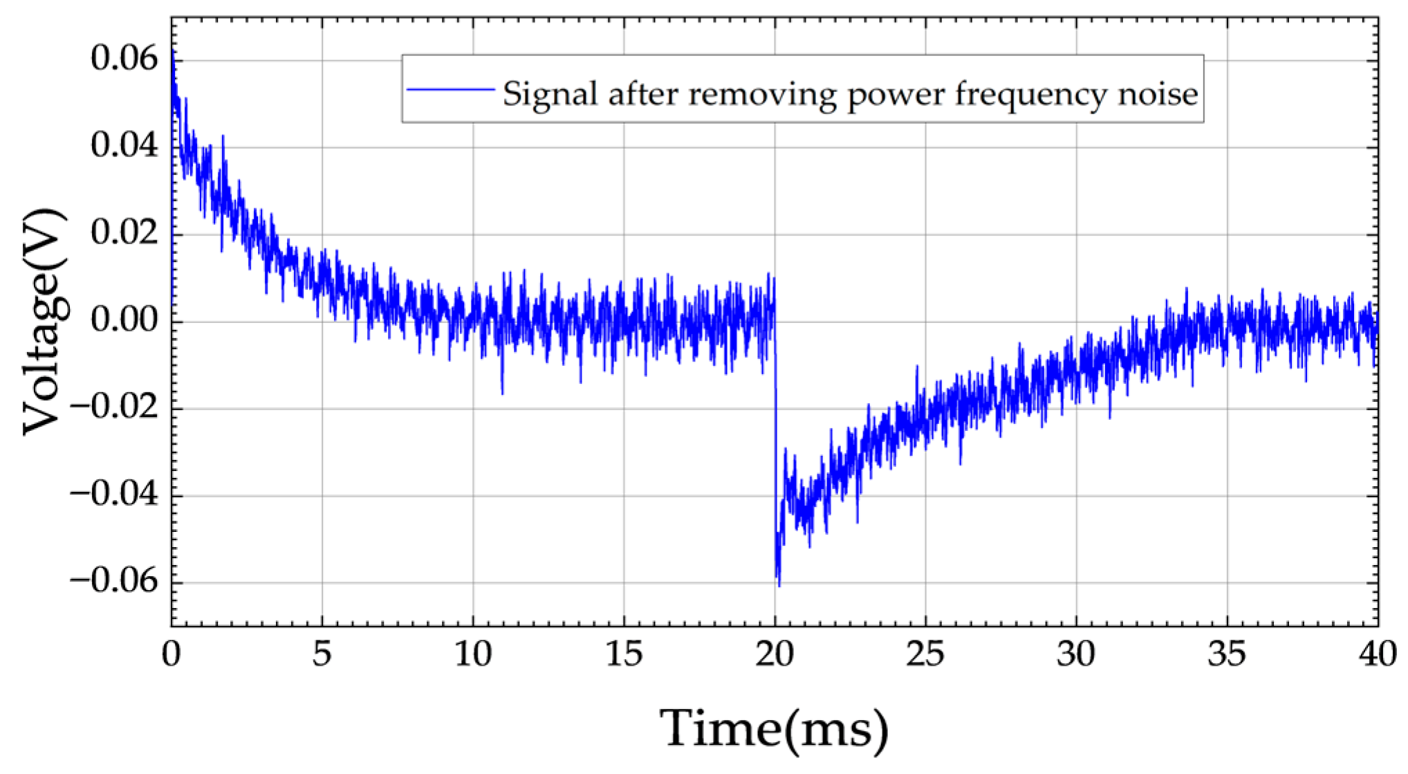
According to the periodic characteristic of power frequency noise, the power frequency noise in electromagnetic signals can be removed. The electromagnetic signals are divided into effective signals and noise signals as follows:

$$v(t)=s(t)+f_n(t)+r_n(t)$$

(1)

where v(t) is the electromagnetic signal collected by the receiving coil; s(t) is the effective electromagnetic signal reflecting the underground medium, and the information contained therein can be used for the subsequent inversion of the substation grounding grid; f_n(t) is the power frequency interference and its harmonics, which are the main processing objects of power frequency filtering; r_n(t) is the random noise collected in the substation.

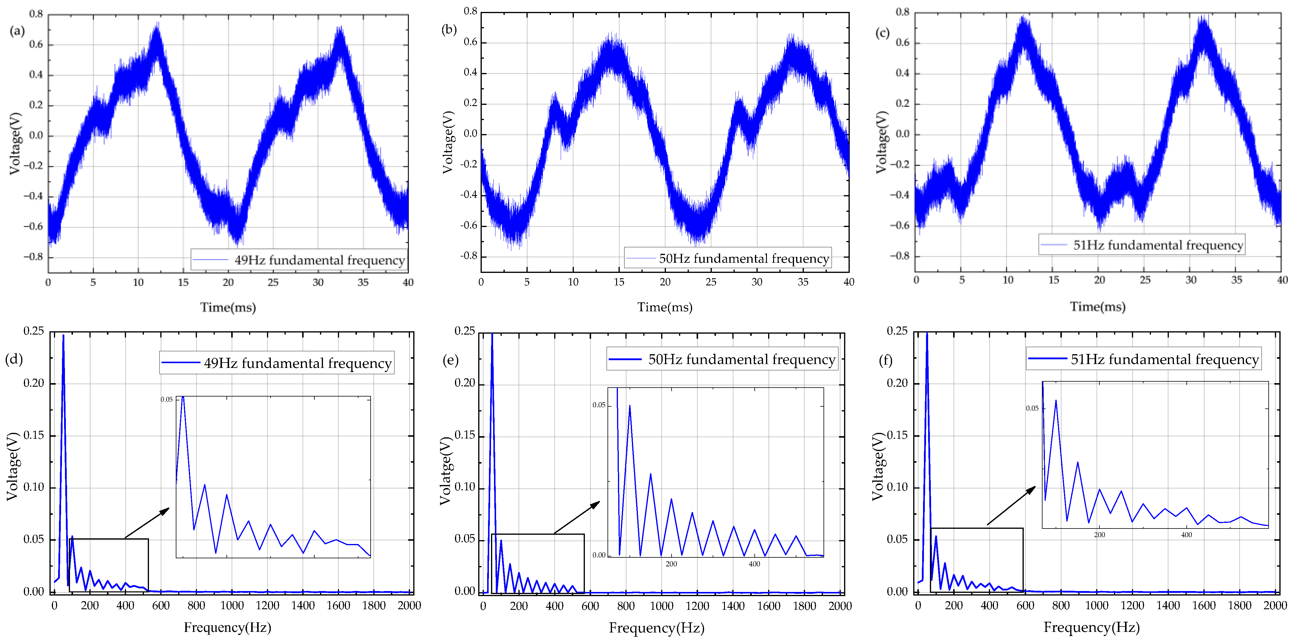
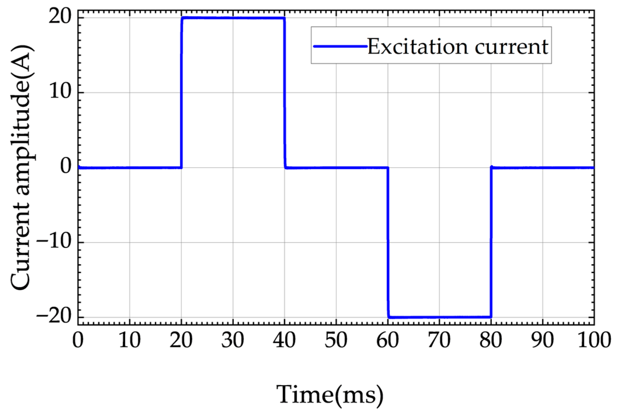
The power frequency interference in the substation is particularly serious. In this paper, the power frequency interference is first suppressed by the method of positive and negative bipolar cancellation. The power frequency interference in Chinese substations is mainly composed of the 50 Hz fundamental frequency and its integer-multiple harmonics. To utilize its periodic characteristics and thereby cancel the power frequency noise through bipolarity, the article sets the excitation frequency of the transmitting coil to 25 Hz with a duty cycle of 25%, and the transmitting waveform is a bipolar pulse square wave. At this time, the signal in a single period can be divided into positive signals and negative signals:

$$\left\{\begin{array}{c}{v}_{+}(m)=s_{+}(m)+f_{n+}(m)+r_{n+}(m)\\ v_{-}(m)=s_{-}(m)+f_{n-}(m)+r_{n-}(m)\end{array}\right.$$

(2)

where v₊(m) and v₋(m) represent first and second half of a PEC periodic signal, respectively, where m denotes the number of signal points collected in one period; s₊(m) and s₋(m) are the positive and negative pulsed electromagnetic signals, respectively, with the same amplitude but opposite directions; f_n+(m) and f_n−(m) refer to the power frequency interference and its harmonics. Since power frequency noise does not change abruptly in a short time, it can be considered that r_n+(m) and r_n−(m) have the same power frequency phase and amplitude. The power frequency interference can be effectively suppressed by performing differential averaging on v₊(m) and v₋(m), as shown in (3).

$$\begin{array}{c}{v}_{out}(m)=v_{+}(m)-v_{-}(m)\\ =s_{+}(m)-s_{-}(m)+r_{n+}(m)-r_{n-}(m)\end{array}$$

(3)

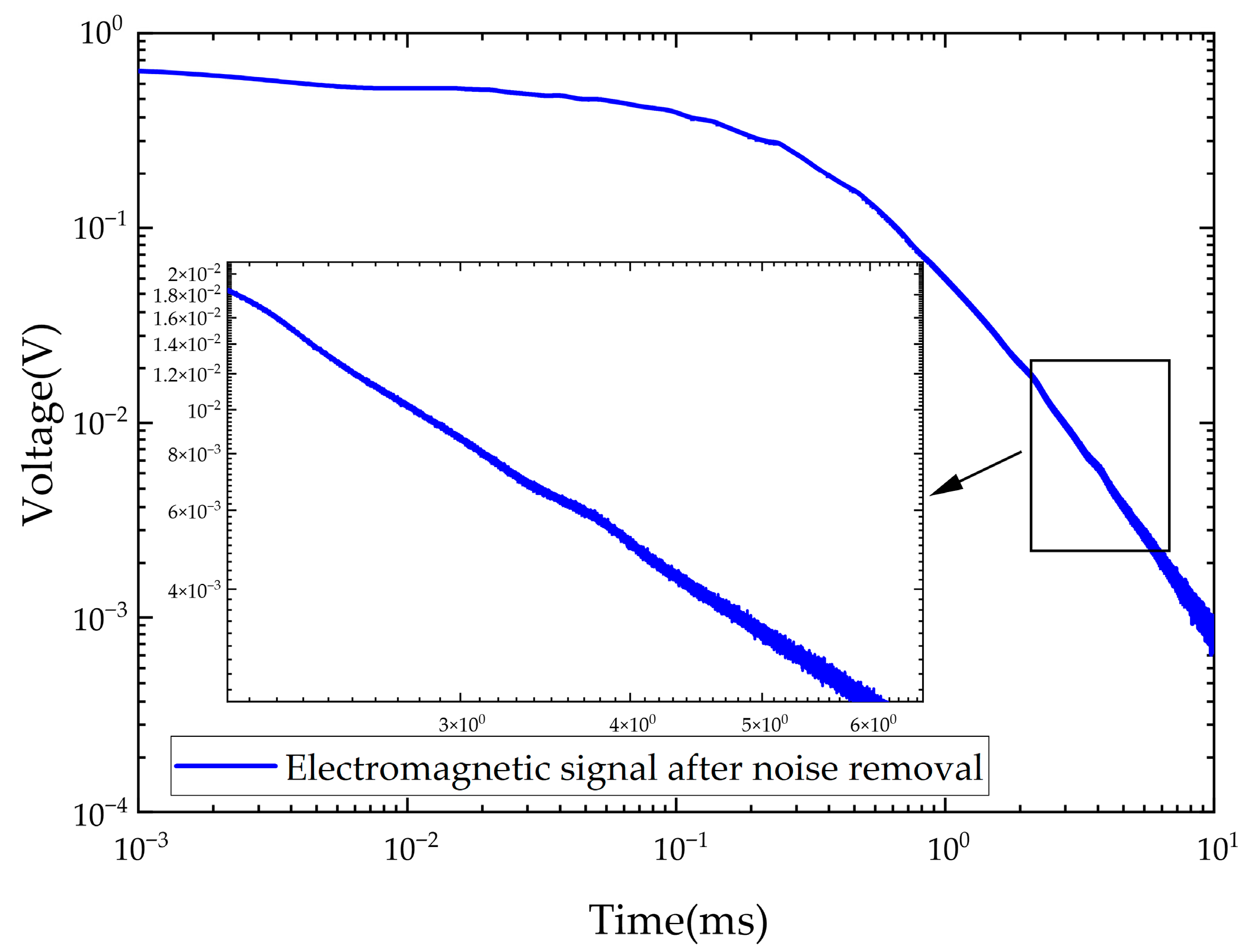
From (3), we can see that the power frequency interference in the electromagnetic signal has been eliminated by using the differential averaging method, but the random noise still remains. For this reason, MNF is further introduced to suppress the random noise.

2.2. PEC Random Noise Suppression Based on MNF

MNF is a noise reduction method based on statistical characteristics, which is often used for noise reduction and signal extraction of high-dimensional data. In this paper, MNF is applied to the random noise processing of PEC data after power frequency interference removal. Through reconstruction with a certain threshold, random noise is separated from effective signals. After the power frequency preprocessing is completed by the above-mentioned bipolar cancellation power frequency filtering method, the collected PEC signal is X(m × n):

$$X=\left[\begin{array}{cccc}{x}_{11}& x_{12}& \dots & x_{1n}\\ x_{21}& x_{22}& \dots & x_{2n}\\ ⋮& ⋮& \ddots & ⋮\\ x_{m1}& x_{m2}& \dots & x_{mn}\end{array}\right]=X_S+X_R$$

(4)

where X is the noisy data with effective signal X_S and random noise X_R. In addition, X_S and X_R are independent of each other. Here, n represents n cycles, and m is the number of datapoints contained in a single cycle; the covariance matrix C corresponding to X can be decomposed into the signal matrix C_S and the noise matrix C_R:

$$C=C_S+C_R$$

(5)

The C_R is calculated by the maximum autocorrelation factor algorithm, where C_R is composed of elements γ_kq.

$$\left\{\begin{array}{l}{\gamma }_{kq}=0.5{\displaystyle \frac{1}{n-1}}{\displaystyle \sum _{i=1}^{n-1}}(z_k(j)-{\overline{z}}_k)(z_q(j)-{\overline{z}}_q)\\ z_k(j)=x_k(j+1)-x_k(j)\\ z_q(j)=x_q(j+1)-x_q(j)\end{array}\right.$$

(6)

where z_k(j) and z_q(j) represent the differences between the (j + 1)-th group of signals and the j-th group of signals in the k-th and q-th channels of data, respectively, while ${\overline{z}}_k$ and ${\overline{z}}_q$ are the average values of the k-th and q-th channels of data, respectively. In (6), k, q = 1, 2, …, n; j = 1, 2, …, m − 1; the C_R is decomposed into the following formula by singular value decomposition:

$$C_R=U{D}_R{U}^T$$

(7)

where D_R is a diagonal matrix of eigenvalues, and U is a vector matrix corresponding to the eigenvalues. Construct the transformation matrix P:

$$P=U{D}_R^{-1/2}$$

(8)

And X is adjusted to XP, which lead to noise variance in minimum noise component of the PEC is a unit variance. Through calculation, the relationship between the covariance matrix C_X of the transformed data XP and C of original data X in (9):

$$C_X=P^{T}CP=V{D}_X{V}^T$$

(9)

In (9), the covariance matrix C_X is subjected to singular value decomposition, resulting in D_X and V, where these two matrices are the eigenvalue matrix and eigenvector matrix, respectively. The second transformation matrix W = PV is constructed using the transformation matrix P and the eigenvector matrix V, and the PEC data X is linearly transformed using matrix W to obtain the MNF matrix ψ.

$$\psi =W^{T}X=\left[\begin{array}{c}{\psi }_1\\ {\psi }_2\\ ⋮\\ {\psi }_m\end{array}\right]$$

(10)

The MNF in matrix ψ is defined as the ratio of the noise variance in the data to the variance of the data itself, and formula is (11):

$$NF={\displaystyle \frac{\mathrm{var}(R)}{\mathrm{var}(S+R)}}$$

(11)

In (11), a smaller NF indicates a larger ratio of the effective signal to the total signal. Moreover, since the MNF transformation is a linear transformation, the PEC data X can be reconstructed using the MNF matrix. When a certain number of components are selected for reconstruction, the original PEC data X can be well recovered.

The MNF matrix is arranged in descending order of the effective signal ratio. The front principal components mainly contain the effective PEC signal Xs, with the noise component X, being secondary, while the rear principal components are dominated by noise X_P, with the effective signal X_S being secondary. Therefore, random noise can be effectively suppressed by reasonably selecting a small number of MNFs with high effective signal ratios for reconstruction, as shown in (12).

$$X_s=\left[\begin{array}{c}{\psi }_1\\ ⋮\\ {\psi }_a\\ 0\\ ⋮\\ 0\end{array}\right],X_R=\left[\begin{array}{c}0\\ ⋮\\ 0\\ {\psi }_{a+1}\\ ⋮\\ {\psi }_m\end{array}\right]$$

(12)

In (12), the effective PEC signal X_S is reconstructed by selecting the first MNFs, while the MNFs from a−1 to m correspond to the random noise component Xp of data.

The components after MNF transformation are arranged in descending order of signal-to-noise ratio. Therefore, the essence of determining the reconstruction threshold a is to distinguish between signal-dominated components and noise-dominated components. To enhance the reproducibility of the method, this paper adopts the cumulative contribution rate method to determine the threshold a. Specifically, the eigenvalue λ_i of each component in the minimum noise component matrix ψ is first calculated. The eigenvalue reflects the energy contained in the component. Then, the cumulative energy contribution rate C_k of the first k components is calculated:

$$C_k={\displaystyle \frac{{\displaystyle \sum _{i=1}^k{\lambda }_i}}{{\displaystyle \sum _{i=1}^m{\lambda }_i}}}$$

(13)

By setting a cumulative contribution rate threshold T = 95%, the threshold a is determined to be the minimum integer that satisfies C_a ≥ T. This method can adaptively retain most of the effective signal energy while discarding the remaining components dominated by noise, thereby achieving effective random noise suppression under the premise of ensuring signal fidelity.

Because the noise signal and the effective signal are independent of each other, MNF achieves the suppression of random noise through the following process: (1) Take input data into orthogonal components sorted in descending order of the effective signal ratio; (2) Select some components with higher effective signal ratios for signal reconstruction; (3) Effectively separate and remove noise components with lower effective signal ratios. This process can reduce the prediction pressure of the subsequent convolutional neural network and improve the noise reduction accuracy.

2.3. Residual Noise Suppression Based on Mask Guidance

After MNF processing, we propose a deep neural network which used to study sparse representation of signals and train a nonlinear mapping function. This function converts the sparse representation of data into a mask, thereby decomposing the input data into target signals and noise. The theory behind sparse representation-based noise reduction lies in the fact that natural image signals can usually be sparsely represented, while noise does not have this property. Therefore, the problem of separating noise signals from effective signals is modeled as a supervised learning problem. Specifically, by predicting the semantic mask of effective electromagnetic signals, the proportion of effective signals at each data point is determined, so as to achieve noise reduction.

2.3.1. Segmentation Convolutional Neural Network

The noisy signal processed by MNF is denoted as Y(m, n), which consists of two parts: the effective electromagnetic signal S(m, n) and the noise signal N(m, n).

$$Y(m,n)=S(m,n)+N(m,n)$$

(14)

Inspired by the autoencoder’s ability to learn sparse representations of data, a FCNN architecture is designed in Figure 1, which includes a progressively contracting encoder and a progressively expanding decoder to effectively extract and recover key features of the signal. To further improve the training convergence speed and prediction performances kip connections are introduced to retain more critical information during the encoding and decoding processes. In this network diagram, a deep neural network is employed to model and learn the expressive features of the signal and noise. This structure draws inspiration from Wiener Deconvolution, aiming to characterize the effective signal and noise components with as few non-zero elements as possible by seeking sparse representations. The network learns two masks to achieve effective separation of the signal and noise:

$$\left\{\begin{array}{l}{M}_S\left(m,n\right)=\left({\displaystyle \frac{1}{1+\frac{\left|N\left(m,n\right)\right|}{\left|S\left(m,n\right)\right|}}}\right)\\ M_N\left(m,n\right)=\left({\displaystyle \frac{\left|N\left(m,n\right)\right|}{1+\frac{\left|N\left(m,n\right)\right|}{\left|S\left(m,n\right)\right|}}}\right)\end{array}\right.$$

(15)

where M_S(m, n) and M_N(m, n) are the masks of the effective signal S(m, n) and the noise signal N(m, n), respectively. Both the masks of the effective signal and the noise signal have the same size as the input matrix, and their values range between 0 and 1, which are used to attenuate the input matrix to obtain effective and noise signal.

The first layer in the block diagram takes the data matrix after time-channel decimation as input, and the last layer yields masks for the effective signal and noise signal for subsequent signal processing. The input data matrix is processed and transformed through a series of 2D convolutional layers, which employ ReLU activation functions and are trained with batch normalization. The first layer of the block diagram inputs the data matrix after time-channel processing, followed by a downsampling module for signal feature extraction. The convolution kernel is fixed at 3 × 3, and the feature space is gradually reduced through a 2 × 2 stride. Eventually, a sparse representation of the input data is learned in the bottleneck layer, where the number of convolution kernel channels is 8, 8, 8, 16, 1632, 32, 64, 64, 128, 128, 256 respectively, with 256 being the number of channels in the bottleneck layer. The latter half of the block diagram primarily restores the feature map to its original size through deconvolution, and finally generates masks via Softmax normalization, ensuring the sum of the two masks is 1. The number of convolution kernel channels here is 256, 128, 128, 64, 64, 32, 32, 16, 16, 8, respectively. The final output consists of two lavers of masks representing the noise signal and the effective signal. During training, cross-entropy loss is introduced to continuously optimize and learn the optimal masks and skip connections are incorporated to create direct links between the downsampling and upsampling paths of the deep network, preventing information loss. Unlike traditional methods that rely on manually setting feature parameters and thresholds to enhance signals and suppress noise, this deep neural network can automatically learn richer feature representations from semi-real electromagnetic data thereby achieving the separation of effective signals and noise. The specific parameters are shown in the following

Table 1. Architecture Parameters of Segmentation Convolutional Neural Network.

Network Stage	Layer Type	Layer Index	Kernel Size	Number of Kernels	Activation Function	Stride	Output Dimension
Encoder (Downsampling)	Input Layer	Input	6.53	-	-	-	64 × 64 × 1
	Convolutional Layer	Conv1	3 × 3	8	ReLU	-	64 × 64 × 8
	Convolutional Layer	Conv2	3 × 3	8	ReLU	-	64 × 64 × 8
	Max Pooling Layer	Pool1	2 × 2	-	-	-	32 × 32 × 8
	Convolutional Layer	Conv3	3 × 3	16	ReLU	-	32 × 32 × 16
	Convolutional Layer	Conv4	3 × 3	16	ReLU	-	32 × 32 × 16
	Max Pooling Layer	Pool2	2 × 2	-	-	-	16 × 16 × 16
	Convolutional Layer	Conv5	3 × 3	32	ReLU	-	16 × 16 × 32
	Convolutional Layer	Conv6	3 × 3	32	ReLU	-	16 × 16 × 32
	Max Pooling Layer	Pool3	2 × 2	-	-	-	8 × 8 × 32
	Convolutional Layer	Conv7	3 × 3	64	ReLU	-	8 × 8 × 64
	Convolutional Layer	Conv8	3 × 3	64	ReLU	-	8 × 8 × 64
	Max Pooling Layer	Pool4	2 × 2	-	-	-	4 × 4 × 64
Bottleneck Layer	Convolutional Layer	Bott1	3 × 3	128	ReLU	-	4 × 4 × 128
	Convolutional Layer	Bott2	3 × 3	256	ReLU	-	4 × 4 × 256
Decoder(Upsampling)	Transposed Convolutional Layer	Deconv1	2 × 2	128	ReLU	-	8 × 8 × 128
	Convolutional Layer	Conv9	3 × 3	64	ReLU	-	8 × 8 × 64
	Convolutional Layer	Conv10	3 × 3	64	ReLU	-	8 × 8 × 64
	Transposed Convolutional Layer	Deconv2	2 × 2	32	ReLU	-	16 × 16 × 32
	Convolutional Layer	Conv11	3 × 3	32	ReLU	-	16 × 16 × 32
	Convolutional Layer	Conv12	3 × 3	32	ReLU	-	16 × 16 × 32
	Transposed Convolutional Layer	Deconv3	2 × 2	16	ReLU	-	32 × 32 × 16
	Convolutional Layer	Conv13	3 × 3	16	ReLU	-	32 × 32 × 16
	Convolutional Layer	Conv14	3 × 3	16	ReLU	-	32 × 32 × 16
	Transposed Convolutional Layer	Deconv4	2 × 2	8	ReLU	-	64 × 64 × 8
	Convolutional Layer	Conv15	3 × 3	8	ReLU	-	64 × 64 × 8
	Convolutional Layer	Conv16	3 × 3	8	ReLU		64 × 64 × 8
	Output Layer	Output	1 × 1	2	Softmax		64 × 64 × 2

.

2.3.2. Loss Function

In segmentation DNN, the loss function mainly consists of two parts: the signal mask loss and the noise mask loss, which are jointly optimized using the cross-entropy loss function. When the model has been trained, each point in the input two-dimensional array is predicted as a composition of the effective signal and residual noise, and the network outputs two masks: the signal mask M_S(m, n) and the noise mask M_N(m, n). For each sampling point, its true label is given by the signal mask M_S(m, n) and the noise mask M_N(m, n), which are used in the supervised learning process. The L_mask is defined in (15):

$$L_{mask}(M_S,M_N,Y_S,Y_N)=-{\displaystyle \sum _{m,n}[Y_S(m,n)\log M_S(m,n)+Y_N(m,n)\log M_N(m,n)]}$$

(16)

where M_S(m, n) and M_N(m, n) are the predicted effective signal mask and noise mask, respectively. Y_S(m, n) and Y_N(m, n) are the real signal mask and noise signal mask, respectively. The loss function L_MASK of the model is composed of the effective signal mask loss and the residual noise mask loss:

$$L_{MASK}={\displaystyle \frac{1}{MN}}{\displaystyle \sum _{m,n}{L}_{mask}(M_S,M_N,Y_S,Y_N)}$$

(17)

where M and N are the total numbers of sampling time points and channels, respectively, ensuring that the loss is evenly distributed across the entire channel. The goal of the segmentation neural network is to minimize this loss function, so that the predicted signal mask M_S(m, n) approaches the real signal mask Y_S(m, n), and the predicted noise mask M_N(m, n) approaches the real noise mask Y_N(m, n), thereby achieving accurate separation of signal and noise. L_MASK measures the matching degree between the model-predicted signal/noise masks and the ground-truth masks obtained from forward simulations. It directly corresponds to three key denoising effects: (1) Preventing late-stage weak PEC signals (critical for grounding grid inversion) from being misclassified as noise and discarded; (2) Only suppressing residual noise in a targeted manner without damaging valid signals; (3) Ensuring consistent denoising performance of the model in both early-stage strong signal segments and late-stage weak signal segments.

3. Construction of Random Noise Suppression Model

3.1. Generation and Processing of Training Dataset

To generate the training-labeled data required for model training, this study collected a large amount of pulsed eddy current forward modeling data by performing batch forward modeling on a broadly representative substation grounding grid model. This data served as the foundation for network training. The forward model parameters were not selected based on a single site; but rather were designed to cover a wide range of scenarios in typical substation grounding grids in China, ensuring the generalizability of the method.

The forward modeling of the grounding grid in this study was developed and solved using COMSOL Multiphysics 6.1. The simulation calculation model is shown in Figure 2 and consists of a five-layer soil structure. The grounding conductor (the third layer) is made of galvanized steel with a resistivity of 1 × 10⁻⁶ Ω·m. Its burial depth was randomly generated between 0.6 m and 2 m to cover regulatory requirements and common practical conditions. The resistivity of the upper dielectric layers (the first and second layers) was randomly set between 100 and 600 Ω·m to simulate different geological conditions, ranging from dry soil to moist clay. The layer thicknesses were randomly generated, but the total thickness equaled the grounding conductor burial depth. In the underlying medium, the fourth layer is fixed at 1 m thick, and the fifth layer is a semi-infinite space. The resistivities of both layers are uniformly and randomly distributed within the range of 100–1000 Ω·m to reflect the randomness of the underground layered structure. Based on these parameter settings, a total of 100,000 geoelectric models with different parameter combinations were generated, and pure pulsed eddy current signals were obtained as label data through forward calculations.

To construct a noisy training dataset that closely resembles real-world scenarios, we designed a synthetic process based on measured noise modeling. We collected real-world background electromagnetic noise samples from equipment operating in typical substations at various voltage levels (including 110 kV and 220 kV). These samples were analyzed and categorized into three types: power frequency harmonic noise, random spike noise, and broadband Gaussian noise. The power frequency noise has a fundamental frequency of 50 Hz and contains up to 15 harmonics. The amplitude of each harmonic is randomly set between 0.1 and 1.0 times the fundamental amplitude, which is 0.2 to 0.8 times the signal peak. The initial phase is randomly distributed between 0 and 2π. The amplitude of the random spike noise is 1.5 to 5 times the original signal peak, with a probability of occurrence set between 1% and 5%. The signal-to-noise ratio of the broadband Gaussian noise ranges from 0 dB to 20 dB to simulate a variety of real-world interference scenarios, from strong to weak. The pure forward modeled signal is linearly superimposed with three types of noise in random proportions, with the signal-to-noise ratio (SNR) used as the key control variable to ensure that the synthetic data covers a wide range of SNR conditions from −5 dB to 25 dB. This process combines large-scale forward modeling with extensive field-measured noise modeling to ensure that the proposed noise reduction method is adaptable to diverse substation environments, avoiding overfitting to specific scenarios and ultimately forming an effective solution to universal noise problems.

3.2. Model Training

The He Normal initialization method is adopted to set the network parameters for optimizing the weight distribution. To improve the efficiency of model training, the initial learning rate is 0.01 and adynamic learning rate decay strategy is employed for adaptive optimization. During the training process after every 100 epochs, the learning rate is adjusted to 0.1 times its original value, so as to reduce the oscillation amplitude of the model during the late period of training, stabilize convergence process, and avoid the impact of gradient explosion on model performance. In overall process, the number of epochs is 600. Meanwhile, to enhance the efficiency of gradient optimization, the Adam optimizer is selected to accelerate the model convergence speed and improve training stability.

The numerical simulations and model training for this study were performed on a high-performance workstation equipped with an NVIDIA GeForce RTX 4090 GPU (24 GB of video memory), an AMD Ryzen 9 7950X CPU from Manufactured by Advanced Micro Devices in Santa Clara, CA, USA (16 cores), and 64 GB of DDR5 memory. The deep learning framework was based on PyTorch 2.0, with GPU acceleration using CUDA 12.1.

4. Simulation Data Testing

4.1. Power Frequency Noise Suppression

To verify the effectiveness of the proposed bipolar noise suppression method, this section introduces power frequency noise with fundamental frequencies of 49 Hz, 50 Hz, and 51 Hz, respectively, based on the following equations. Gaussian white noise is then superimposed to simulate a complex noise environment. Noise signal generation and data preprocessing were performed in MATLAB R2021b, using the Signal Processing Toolbox 8.2 toolkit to simulate and superimpose power frequency noise, spike noise, and Gaussian white noise.

$$F(t)={\displaystyle \sum _{k=1}^n\cos (2\pi kft+{\varphi }_k)}$$

(18)

where n is the total number of power frequency harmonics, f represents the power frequency used, t denotes time, and ϕ is the initial phase of the harmonics. The rest of the parameter settings are shown in

Table 2. Parameter setting summary table.

Parameter Category	Parameter Name	Parameter Value/Setting	Unit
PEC Reference Signal Parameters	Signal Source	Grounding grid forward model (5-layer stratum, grounding grid burial depth 0.8 m)	-
	Signal Period	40	ms
	Number of Sampling Points per Period	4000	Point
	Signal Peak Amplitude	0.2	V
	Signal Late-stage Amplitude (at 20 ms)	0.05	V
Power Frequency Noise Parameters	Fundamental Frequency (3 groups for comparison)	49, 50, 51	Hz
	Fundamental Wave Amplitude	0.5	V
	Number of Superimposed Harmonics	10 (including 2–11th harmonics)	Time
	Harmonic Amplitude Attenuation Law	Reciprocal of harmonic order (i.e., the amplitude of the nth harmonic = 0.5/n)	V
	Initial Phase of Each Harmonic	Randomly distributed in (0–2π)	Rad
Superimposed Gaussian Noise Parameters	Noise Type	Zero-mean Gaussian white noise	-
	Noise Amplitude (Standard Deviation)	0.05	V
	Noise Superimposition Method	Linearly superimposed with “PEC reference signal + power frequency noise”	-

. According to (18), the signal waveforms of power frequency noise with fundamental frequencies of 49 Hz, 50 Hz, and 51 Hz are obtained, respectively, as shown in Figure 3.

The spectrum analysis results shown in Figure 3 were obtained using a fast Fourier transform (FFT) with a length of 4096 points and a sampling rate of 1 MHz. A Hanning window was used to reduce spectral leakage. The sidelobes shown in the figure are primarily caused by spectral leakage due to windowing, an inherent phenomenon of windowing. Due to the frequency domain quantization effect and the energy diffusion caused by the window function, the fundamental amplitude displayed by the FFT is slightly lower than the nominal amplitude in the time domain, which is consistent with digital signal processing theory. To highlight the key frequency band characteristics, the spectrum display range is limited to the frequency band of interest of 50–500 Hz. Three groups of noise signals are shown in Figure 3, corresponding to fundamental frequencies of 49 Hz, 50 Hz and 51 Hz from top to bottom. The fundamental amplitude of each group of noise signals is set to 0.5 V with 10 harmonic components superimposed, and the initial phase of each component is randomly generated. In addition, Gaussian noise with an amplitude of 0.05 V is superimposed on the original power frequency noise to simulate random interference in the actual environment. The duration of each group of noise signals is 40 ms, which facilitates superposition processing with forward simulation signals. The superimposed signals are shown in Figure 4:

SNR is often used to describe the degree to which valid data is interfered by noise. This paper also uses the SNR to characterize the effectiveness of noise reduction method. The definition of SNR is as follows:

$$SNR=10\times {\log }_{10}({\displaystyle \frac{{\displaystyle \sum _i^{n}s{(i)}^2}}{{\displaystyle \sum _i^{n}f{(i)}^2}}})$$

(19)

where n is the number of sampling points in one cycle of data, s(i) and f(i) represent the ideal signal and the pure noise signal, respectively. The SNRs under each fundamental frequency interference are calculated in

Table 3. SNRs of power frequency noise before noise reduction.

	49 Hz Interference	50 Hz Interference	51 Hz Interference
SNR (dB)	5.84	5.96	6.53

.

At this point, the SNRs of the three differ due to differences in their initial phases resulting in variations in their initial SNR values. Therefore, in the subsequent evaluation of noise reduction effectiveness, the trend of SNR changes will be used to determine the noise reduction effect. After suppression, the final noise reduction results are in Figure 5. The signal-to-noise ratio of the power frequency noise after denoising is shown in

Table 4. SNRs of power frequency noise after denoising.

	49 Hz Interference	50 Hz Interference	51 Hz Interference
SNR(dB)	12.92	17.57	16.44

.

According to the calculation results in Table 3 and Table 4, the SNRs of the 49 Hz, 50 Hz and 51 Hz power frequency electromagnetic signals are increased by 121.23%, 194.79%, and 151.76%, respectively. Under the condition where both Gaussian noise and random phase interference exist, the adopted bipolar power frequency noise suppression method exhibits significant noise reduction effects at each frequency point, and can effectively improve the SNR of the signals.

4.2. Random Noise Suppression

To verify the effectiveness of the proposed method in suppressing random noise, a mixed noise scenario consisting of spike noise, Gaussian white noise, and instrument noise floor was constructed through numerical simulation. The Gaussian white noise was set to zero mean and a variance of 0.1 V². Spike noise was simulated by randomly adding pulses with an amplitude three times the peak value to the original signal, with a probability of 5%. The instrument noise floor was directly captured from the background noise of the actual measurement device in an unstimulated state. Based on this, the performance of the proposed noise reduction method was evaluated and verified. To suppress random noise, spike, Gaussian white, and instrument background noise are selected to construct numerical simulation scenarios, so as to evaluate the performance of noise reduction method. The ideal PEC signals are obtained through the forward model, with the parameter settings in

Table 5. PEC signal forward model parameter settings.

Parameter	Parameter Setting	Parameter	Parameter Setting
Model layer	5	Number of grounding grid layers	The third layer
Grounding grid burial depth	0.8 m	Grounding grid material	Galvanized steel
Resistivity (Ω∙m)	[300, 400, 1 × 10−6, 500, 600]	Model layer thickness	[0.4, 0.4, 0.0012, 1, ∞]

:

By combining the electromagnetic data obtained from the forward model with the generated random signals, the noise superposition effect shown in Figure 6 is obtained. Among them, (a) shows that the spike noise manifests as sudden high-amplitude abnormal points in the time series, and (b) demonstrates that the spike noise presents local mutation characteristics in the time domain of the electromagnetic signal; the Gaussian noise shown in (c) has statistical characteristics of zero mean and constant variance, and (d) indicates that this noise mainly causes significant interference to the late period of the electromagnetic signal; (e) reflects the influence of the time-series fluctuation of the amplitude of the sampling points of the instrument background noise, and (f) shows that this influence is across the entire time domain and has a similar variation pattern to the electromagnetic signal.

After synthesizing the noise, the SNR at this point is 3.1811 dB. A comparative experiment was conducted between several popular electromagnetic noise removal methods and the method proposed. Therefore, a comparison is made with 17-layer DcCNN, wavelet threshold, and F-K filter models. The model parameters are shown in

Table 6. Different model parameter settings.

Denoising Method	Core Parameters	Value/Configuration
DnCNN	Network Layers	17 layers (including 1 input layer, 15 convolutional layers, and 1 output layer)
	Convolution Kernel Size	3 × 3 (for all convolutional layers)
	Activation Function	ReLU (except for the output layer)
	Training Parameters	Batch Size = 16, Learning Rate = 1 × 10−4, Optimizer = Adam, Number of Epochs = 100
	Noise Adaptation	Trained only for Gaussian noise (no power frequency noise samples introduced)
Wavelet Thresholding	Wavelet Basis Function	db4 (Daubechies 4 Wavelet)
	Decomposition Levels	5 levels
	Threshold Rule	Soft Thresholding
	Threshold Calculation Method	Automatically calculated based on Stein’s Unbiased Risk Estimate (SURE)
F-K Filtering	Frequency-Wavenumber Domain Conversion Parameters	Number of Sampling Points = 4000 (consistent with PEC signal sampling rate), Window Function = Hanning Window (suppresses spectral leakage)
	Filtering Threshold (Wavenumber)	0.8 cycles/m (only signal components with wavenumber < 0.8 are retained)
	Phase Correction Method	Linear Phase Correction

, and the noise reduction results are shown in Figure 7.

In the comparative experiments, to ensure fairness, all the comparison methods used typical or original recommended parameter settings. The wavelet threshold method used the “db8” wavelet basis function, with a decomposition layer number of 5 and a threshold value of 0.1. The DnCNN model [24] used its standard 17-layer structure, containing 64 convolutional filters of size 3 × 3, and used the Adam optimizer for prediction; this model has been pre-trained in image denoising tasks and can be directly transferred for one-dimensional signal denoising. The F-K filter [25] sets the tilt threshold range to −0.05 to 0.05 ms/m, suppressing the visual tilt components outside this range to achieve noise filtering. To evaluate the robustness and repeatability of the method, a total of 200 randomly generated geoelectric models were used as test samples in this simulation test. The noise addition and noise reduction processes for each model were repeated 10 times independently. The final results show the average SNR of all test samples and repeated tests. The obtained results are in

Table 7. SNR of denoised PEC signals from different models.

	Paper	DnCNN	Wavelet	F-K Filter
SNR(dB)	5.84	5.96	6.53	37.8

.

The simulation results in Figure 8 show that, compared to traditional noise reduction methods, the proposed random noise suppression method achieves the highest degree of overlap between the processed PEC signal and the ideal signal, better approximating the theoretical PEC signal. Furthermore, the data in Table 7 further demonstrates that the proposed method significantly outperforms the other compared methods in terms of SNR, demonstrating superior noise suppression performance. To verify the role and necessity of bipolar cancellation, MNF, and mask-guided CNN, the contribution of each step to the SNR improvement is quantified as shown in the following

Table 8. Contribution of different methods to SNR during actual measurement.

Processing Stage	Simulated Data SNR (dB)	Improvement over the Previous Stage
Original Noisy Signal (Unhandled)	5.96	-
Only Bipolar Cancellation Processing	12.83	SNR + 114.9%
Bipolar Cancellation + MNF Processing	14.65	SNR + 14.2%
Full-Process Processing (Combination of Three Steps)	17.57	SNR + 20.0%

.

The improvement in each step shows that bipolar cancellation contributes the most to the SNR increase (+114.9%) and is the core of suppressing strong power frequency noise. MNF and mask-guided CNN improve SNR by +14.2% and +20.0%, respectively, gradually addressing the issues of random noise and residual overlapping noise.

5. Experimental Testing

In this paper, signal collection is performed on a substation in a certain region of China using a PEC device. The collection method is point collection, with a total of 50 measurement points set up. That is, measurements are taken every 0.5 m, and each measurement point should collect data for at least 100 cycles. The on-site measurement diagram is shown in Figure 8a. The PEC detection equipment used in this study is a self-developed substation grounding grid PEC detector. The system consists of a transmitter, receiver, control, and auxiliary modules. The transmitter module utilizes a 30-turn copper coil with a radius of 0.4 m, a maximum transmit current of approximately 20 A, and a 25 Hz double-pulse square wave excitation waveform (25% duty cycle) with an off-time of less than 20 μs. The receiver module consists of a 300-turn copper coil with a radius of 0.1 m, a sampling rate of 1 MHz, and a 16-bit A/D converter. The control module is based on an STM32H743 microcontroller from Chinese Dot Atoms, which implements timing synchronization between transmit and receive, as well as data caching, with a storage capacity of 8 GB. A Lenovo ThinkPad laptop was used as an auxiliary device for data storage and preliminary verification during the field experiments. The schematic diagram of the detection device is in Figure 8b.

The excitation waveform after setting the excitation parameters is shown in Figure 9.

Two arbitrary cycles of raw data are in Figure 10 below, which shows the raw signals in Figure 10 that electromagnetic signals containing grounding grid information have been severely distorted.

The article filters out the power frequency noise using the bipolar cancellation power frequency filtering method, and the PEC signal within one cycle at this point is shown in Figure 11:

After using the bipolar power frequency noise suppression method, the proposed method is applied to remove collected random noise, and the signal after noise removal is shown in Figure 12:

It can be seen from Figure 12 that after processing the noise collected from the substation according to the electromagnetic noise suppression strategy proposed in this paper, the measurement results consistent with the ideal signal waveform are obtained. The waveform has high prediction accuracy in all stages and performs extremely well in the prediction of late signals, which are more concerned in PEC inversion. After denoising the experimental data using the method proposed in this paper, the signal-to-noise ratio (SNR) of the signal before and after processing is calculated. The results show that after processing, the average signal-to-noise ratio of the signal increases from 20 dB to 25 dB, significantly increased by 5 dB, which proves the excellent noise reduction performance of the method proposed in this paper in the real substation environment.

6. Conclusions

In this paper, a phased composite noise reduction method is proposed to address the problem that the pulse eddy current method is susceptible to strong electromagnetic interference in substation grounding grid detection. Its effectiveness is verified through simulation and actual measurement. The main conclusions and research contributions are as follows:

(1)

The bipolar cancellation preprocessing stage fully utilizes the periodic characteristics of power frequency noise and effectively suppresses the 50 Hz fundamental and its harmonic components through differential averaging. This method has high computational efficiency and can significantly improve the signal-to-noise ratio in the early stage, providing a cleaner input signal for subsequent processing.

(2)

The minimum noise separation stage adaptively selects the dominant component of the signal for reconstruction based on the cumulative contribution rate threshold, achieving preliminary separation and suppression of random noise. This stage effectively reduces the interference of random components in the data and reduces the burden of the deep network in subsequent noise reduction tasks.

(3)

The mask-guided self-supervised noise reduction stage uses a segmented convolutional neural network to automatically learn the mask of the signal and noise from the data, achieving fine separation of residual noise, especially showing better recognition and fidelity capabilities in the overlapping part of the effective signal frequency band. This stage significantly improves the fidelity of late-stage weak signals, providing reliable support for high-precision inversion of grounding grid parameters.

Simulation and measurement results show that the proposed method outperforms traditional algorithms such as DnCNN, wavelet thresholding, and F-K filtering in terms of signal-to-noise ratio improvement and waveform fidelity, effectively verifying the effectiveness and superiority of the proposed staged composite denoising strategy. Although the current method has achieved good noise reduction results, there is still room for improvement in many aspects. Future work will focus on optimizing the algorithm to reduce computational complexity and build a lightweight network structure; suppressing the risk of overfitting and combining transfer learning strategies to enhance the generalization ability of the model in different substation environments and other scenarios; developing denoising strategies that are insensitive to hardware differences; or building a universal model that can adapt to multiple configurations. In addition, there are plans to advance from the system architecture level, upgrading the current open-loop feedforward processing structure to an intelligent closed-loop system with an online error feedback mechanism, thereby continuously improving the intelligence level and robustness of the denoising process.