Abstract
Accurate load forecasting of central air conditioning (CAC) systems is crucial for enhancing energy efficiency and minimizing operational costs. However, the complex nonlinear correlations among meteorological factors, water system dynamics, and cooling demand make this task challenging. To address these issues, this study proposes a novel hybrid forecasting model termed IWOA-BiTCN-BiGRU-SA, which integrates the Improved Whale Optimization Algorithm (IWOA), Bidirectional Temporal Convolutional Networks (BiTCN), Bidirectional Gated Recurrent Units (BiGRU), and a Self-attention mechanism (SA). BiTCN is adopted to extract temporal dependencies and multi-scale features, BiGRU captures long-term bidirectional correlations, and the self-attention mechanism enhances feature weighting adaptively. Furthermore, IWOA is employed to optimize the hyperparameters of BiTCN and BiGRU, improving training stability and generalization. Experimental results based on real CAC operational data demonstrate that the proposed model outperforms traditional methods such as LSTM, GRU, and TCN, as well as hybrid deep learning benchmark models. Compared to all comparison models, the root mean square error (RMSE) decreased by 13.72% to 56.66%. This research highlights the application potential of the IWSO-BiTCN-BiGRU-Attention framework in practical load forecasting and intelligent energy management for large-scale CAC systems.
1. Introduction
1.1. Background and Significance
As the global climate change crisis intensifies, green and low-carbon development, energy conservation, emission reduction, and sustainable growth have become the dominant themes in today’s world economy. China’s 14th Five-Year Plan explicitly states the nation’s commitment to peak carbon emissions by 2030 and achieve carbon neutrality by 2060 [1]. Realizing these goals requires concerted efforts across all sectors of society, with the construction industry playing a particularly critical role in energy conservation and emission reduction.
Air conditioning energy consumption accounts for a significant portion of China’s total energy load, representing a high-energy-consumption, high-emission industry [2]. With China’s sustained economic growth, air conditioners have become commonplace in households, exhibiting high usage rates during both winter and summer. Particularly during summer, air conditioning loads can constitute 30–40% of total loads in major cities, reaching over 50% in first-tier cities like Shanghai [3,4,5]. Such substantial loads place immense pressure on grid operations. Conversely, air conditioners exhibit low sensitivity to short-term interruptions (for example, they can be temporarily shut down or adjusted while maintaining indoor temperatures within comfortable ranges), endowing them with the potential to serve as a flexible, adjustable resource. Therefore, through effective technical means to aggregate and manage air conditioning loads, they can be transformed from mere “power consumers” into “power regulators” capable of providing substantial regulation capacity to the power system. This regulation capability is crucial for grid peak shaving and valley filling, maintaining stability, and has become a key consideration in grid dispatch [6]. Consequently, accurately assessing the scale of air conditioning loads and their regulation potential is paramount, making it the subject of this study.
1.2. Literature Review
Methods for central air conditioning load forecasting can be broadly categorized into two types: physics-based modeling approaches [7,8,9] and data-driven approaches. Physics-based methods predict loads by establishing thermodynamic models or energy balance equations for buildings, focusing on modeling using physical characteristics and environmental parameters. These methods do not rely on historical data, possess clear physical significance, and are suitable for new buildings or scenarios with limited data. However, they involve higher modeling complexity and may introduce inaccuracies due to simplifications of building dynamic behavior. These methods do not rely on historical data, possess clear physical significance, and are suitable for new buildings or scenarios with scarce data. However, they involve high modeling complexity, and simplifications of building dynamic characteristics may affect accuracy [10]. In contrast, data-driven approaches analyze historical data using statistical or machine learning techniques to capture complex relationships between loads and influencing factors. They can handle nonlinear problems with high prediction accuracy and are primarily categorized into three types: regression statistical methods, machine learning methods, and deep learning methods. Regression analysis is one of the earliest data-driven methods applied in central air conditioning load forecasting. Its core principle involves establishing mathematical relationships between input variables (such as temperature, humidity, and time) and output variables (load) to generate predictions. Common regression techniques include linear regression, multiple linear regression, and nonlinear regression (e.g., polynomial regression).
Reference [11] proposed an improved office building cooling load prediction model based on multiple linear regression. By processing meteorological factors through principal component analysis (PCA), incorporating the cumulative effect of high temperature (CEHT), and employing a dynamic two-step calibration method, the model significantly enhanced prediction accuracy. Its effectiveness was validated using measured data from two office buildings. Reference [12] proposes a Physical-Based Multiple Linear Regression (PB-MLR) model for hourly cooling load prediction in buildings. The model is further optimized through online training and calibration methods, demonstrating strong generalization capability under small-sample learning, short training time, and high interpretability. It is suitable for buildings with insufficient information or varying load patterns. Reference [13] proposes a thermal load prediction model based on ensemble weather forecasting. By incorporating dynamic weather uncertainty and autoregressive methods, it achieves dynamic prediction of thermal loads for district heating systems and applies this to the optimized operation of heat exchange stations. Reference [14] proposes a cooling load prediction model based on multivariate nonlinear regression. Key variables are selected through sensitivity analysis, and prediction accuracy is enhanced by integrating calibration methods. The model is ultimately applied to optimize the CAC system operation of a library, validating its effectiveness and accuracy in practical applications. Reference [15] proposes a time- and temperature-indexed Autoregressive with Exogenous Inputs (ARX) model for predicting hourly thermal loads in buildings. By integrating distinct indices for time intervals and ambient temperatures, this model enhances prediction accuracy and demonstrates its applicability across multiple benchmark building types for both heating and cooling scenarios. Although regression statistical methods perform well in simple scenarios, their expressive power is limited, making it difficult to handle complex nonlinear load variations.
Machine learning methods can better capture the nonlinear characteristics and complex patterns of central air conditioning loads by automatically learning patterns from data. Commonly used machine learning methods include Support Vector Machines (SVM), Artificial Neural Networks (ANN), and gradient boosting trees. Reference [16] proposed a time-based building cooling load prediction model based on Support Vector Machines (SVM). By comparing it with the traditional Backpropagation (BP) neural network model, the superiority of the SVM model in prediction accuracy and generalization capability was validated. Reference [17] proposes an artificial neural network (ANN)-based forecasting method for predicting daytime cooling load energy consumption in three campus buildings in Singapore. By classifying energy consumption data as ANN inputs, the model achieves high accuracy in forecasting future 20-day energy consumption with good recursive properties. Reference [18] proposes an XGBoost-based machine learning model for predicting residential building cooling energy consumption. By integrating weather data, building characteristics, and user electricity bill information, the model demonstrates strong performance across datasets from multiple climate zones. Reference [19] proposes a Gradient-Boosted Decision Tree (GBDT)-based cold load prediction model for ice storage air conditioning systems. Input variables are selected via Pearson correlation analysis, while model hyperparameters are determined using grid search and cross-validation. Experimental results demonstrate high prediction accuracy across diverse load patterns. Reference [20] proposes a LightGBM-based building cooling load prediction method. It employs KNNImputer to impute missing data, 3-sigma processing for outliers, and extends temporal and climatic features. This approach significantly improves prediction accuracy when combined with preprocessed data, outperforming both unprocessed data and BP neural networks. Machine learning methods strike a good balance between predictive accuracy and computational efficiency, capable of handling medium-sized datasets while demonstrating strong generalization capabilities. However, as data scales continue to grow and predictive tasks become more complex, traditional machine learning approaches may face challenges when Deep learning methods can automatically extract high-level features from data through multi-layer neural network structures, making them particularly suitable for processing large-scale, high-dimensional air conditioning load data. Commonly used deep learning methods include Convolutional Neural Networks (CNN), Recurrent Neural Networks (RNN), Long Short-Term Memory (LSTM), and Gated Recurrent Units (GRU). Reference [21] investigated building thermal load forecasting by comparing seven shallow machine learning algorithms, two deep learning algorithms, and three heuristic prediction methods, finding that LSTM demonstrated superior performance in one-hour short-term forecasting. Reference [22] proposed a hybrid model combining Wavelet Threshold Denoising (WTD) and deep learning (CNN-LSTM) for building cooling load prediction. This model processed raw data via WTD, then extracted spatio-temporal features using CNN and LSTM, significantly improving prediction accuracy. Reference [23] proposes an LSTM model with dual attention mechanisms for predicting cooling loads in different functional zones of shopping malls. Key influencing factors are identified through gray relational analysis, and feature attention and temporal attention mechanisms are integrated to enhance the stability of cooling load predictions. Reference [24] proposes a CRG-Informer deep learning model that enhances multi-step prediction performance for building cooling loads by integrating spatio-temporal features. This model combines Graph Neural Networks (GNN) and the Informer model to extract spatial correlations and long-term temporal dependencies in cooling systems, respectively, and demonstrates its superiority through validation on real office building data processing high-dimensional data and nonlinear relationships.
The integration of intelligent optimization algorithms with machine learning and deep learning provides novel approaches and methodologies for model optimization. Common intelligent optimization algorithms include Genetic Algorithm (GA), Particle Swarm Optimization (PSO), Grey Wolf Optimization (GWO), Whale Optimization Algorithm (WOA), Sparrow Search Algorithm (SSA). Applying these algorithms to hyperparameter tuning, network architecture design, and loss function optimization significantly enhances model prediction accuracy and computational efficiency. Reference [25] proposes a joint prediction model based on Improved Variational Mode Decomposition (IVMD), Whale Optimization Algorithm, and Least Squares Support Vector Machine (LSSVM) for air conditioning system cooling load prediction. By optimizing the regularization parameter and kernel width parameter of the LSSVM model via WOA, combined with IVMD of the cooling load sequence to reduce redundant information in input variables, The final cold load prediction results are obtained through reconstruction and superposition, validating the model’s effectiveness and robustness. Reference [26] proposes a prediction model based on the K-means++ algorithm, Rough Set (RS) theory, and Particle Swarm Optimization-enhanced Deep Extreme Learning Machine (DELM) for air conditioning cooling load forecasting in large commercial buildings. The authors employed the PSO algorithm to optimize the weights and thresholds of the DELM neural network, enhancing prediction accuracy. The model demonstrated high precision in both short-term and medium-term cooling load forecasting. Deep learning models effectively address the challenge faced by traditional regression and shallow machine learning models in fully capturing the complex nonlinear temporal features within load data. However, a single deep learning model often struggles to simultaneously account for both the local detailed features and the global temporal dependencies inherent in load data. While some hybrid models attempt to combine the strengths of different networks, they still fall short in bidirectionally extracting and synergistically integrating temporal features. Furthermore, their hyperparameters often rely on empirical settings or standard optimization algorithms (such as GA and PSO), making them prone to getting stuck in local optima.
Despite significant progress in existing research on central air conditioning load forecasting, several critical challenges remain to be addressed. First, single deep learning models (such as LSTM, GRU, or TCN) often struggle to simultaneously capture both the local detailed features and global long-term dependencies within load sequences. Second, while traditional hybrid models attempt to combine the strengths of multiple networks, they remain inadequate in bidirectional feature extraction and collaborative fusion. Furthermore, their hyperparameters heavily rely on empirical settings or conventional optimization algorithms (like GA or PSO), making them prone to local optima and limiting further performance improvements. To address these challenges, this paper proposes a hybrid forecasting framework integrating the Improved Whale Optimization Algorithm (IWOA), Bidirectional Time Convolutional Network (BiTCN), Bidirectional Gated Recurrent Unit (BiGRU), and Self-Attention (SA) mechanism. This framework utilizes BiTCN to extract multi-scale local temporal features, BiGRU to capture bidirectional long-term dependencies, SA to adaptively weight key temporal steps, and IWOA to optimize model hyperparameters for enhanced generalization. Compared to existing approaches, this model structurally achieves collaborative extraction and fusion of bidirectional, multi-scale features. At the optimization level, it introduces a dynamic dual-mutation mechanism that effectively avoids local optima. Consequently, it significantly enhances prediction stability and robustness while maintaining high accuracy.
1.3. Motivation and Contributions
Bidirectional Temporal Convolutional Network (BiTCN) can capture multi-scale local features (including forward and backward features) of temporal data through dilated convolutions, while Bidirectional Gated Recurrent Unit (BiGRU) can further uncover bidirectional global dependencies across the temporal dimension. thereby enabling bidirectional feature co-optimization during both feature extraction and temporal information processing stages in the BiTCN-BiGRU cascaded architecture. When designing the central air conditioning load forecasting model, this paper primarily employs the BiTCN-BiGRU cascaded architecture and introduces a self-attention mechanism (SA) to dynamically weight features at critical time steps. Concurrently, an improved whale optimization algorithm (IWOA) is used to optimize the model’s hyperparameters, further enhancing its prediction accuracy. The main contributions of this paper are as follows:
- (1)
- A hybrid deep learning framework is constructed by combining BiTCN and BiGRU, where BiTCN extracts multi-scale temporal patterns, and BiGRU captures long-term bidirectional dependencies.
- (2)
- A self-attention mechanism is embedded to assign adaptive weights to critical features, enhancing interpretability and robustness.
- (3)
- An improved whale optimization algorithm is designed to tune hyperparameters of BiTCN and BiGRU, avoiding manual trial-and-error and improving model generalization.
- (4)
- Experiments based on real CAC operation data validate that the proposed model outperforms multiple benchmark methods in terms of prediction accuracy and stability.
2. Methodology
2.1. Bidirectional Temporal Convolutional Networks
Temporal Convolutional Networks (TCNs) are a type of convolutional neural network model for processing time series data proposed by Bai et al. [27] in 2018. It employs a hierarchical stacking of one-dimensional causal convolutional kernels to explicitly capture dependencies between time steps. By integrating dilated convolutions and residual connections, TCN achieves efficient multi-scale feature extraction and stable training of deep networks while preserving temporal causality. Compared to traditional Recurrent Neural Networks (RNNs), TCN enables efficient parallel computation, overcoming RNN’s computational bottlenecks when processing long sequences and effectively capturing long-term dependencies. TCN consists of components such as causal convolutions, dilated convolutions, and residual connections. The following sections provide detailed introductions to these key components:
2.1.1. One-Dimensional Convolution
One-dimensional convolution is a fundamental method for sequence feature extraction. Standard one-dimensional convolution extracts local features and generates an output sequence by applying a fixed-width sliding window operation to the input sequence. The feature at each position in the output is computed as a weighted combination of the corresponding position in the input sequence and its adjacent regions before and after.
2.1.2. Causal Convolution
When addressing time series problems, standard one-dimensional convolutions simultaneously cover the current time step and its adjacent regions through sliding window operations. This characteristic enables capturing local contextual information but also leads to data leakage from the future into the past. Therefore, TCN adopts causal convolutions as its foundational architecture. The one-dimensional causal convolution architecture, ensures the causal nature of the time series through a unidirectional convolution kernel design. The output computation at any time point t relies solely on the input data at time t and earlier. A left-padding strategy limits the kernel’s perception range to historical time steps. Assume the convolution kernel is F = (f1, f2,…, fk), the input sequence is XTCN = (x1, x2,…, xt), and the kernel size is K, then the causal convolution at output time t can be expressed as:
2.1.3. Expansion Convolution
As time-dependent distances increase, standard one-dimensional convolutions require stacking multiple layers to capture long-term dependencies. This leads to a dramatic increase in network depth, triggering issues such as vanishing gradients, redundant parameters, and elevated training complexity. To efficiently capture long-term dependencies, TCNs introduce dilated convolutions. The one-dimensional dilated convolution structure, expands the receptive field by inserting gaps (expanded by the dilation rate d) between elements of the convolution kernel.
2.1.4. Dilated Causal Convolution Structure
Expansion-Causal Convolution is a convolution operation that incorporates expansion operations on top of causal convolution. The structure of one-dimensional expansion-causal convolution is shown in Figure 1. It combines the characteristics of causal convolution and expansion convolution. Compared to traditional causal convolution, expansion-causal convolution achieves a larger receptive field at a lower computational cost while maintaining causality. This design makes it more efficient at capturing long-term dependencies. The dilated causal convolution at output time t can be expressed as:
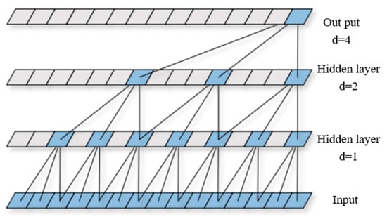
Figure 1.
Dilated causal convolution structure.
2.1.5. Residual Connection
As network depth increases, the network’s ability to capture long-period temporal patterns also improves, but this brings challenges such as gradient vanishing and network degradation. To overcome gradient vanishing and network degradation during deep network training, TCN borrows design concepts from residual networks by introducing residual connections within the causal convolutional expansion modules of each layer. Residual connections establish direct pathways between inputs and outputs, enabling the model to learn residual mappings between inputs and outputs rather than directly fitting the objective function. This significantly improves training stability and feature propagation efficiency in deep networks.
As shown in Figure 2, each residual block of the TCN consists of two paths. The main path includes two layers of dilated convolutions, each followed by weight normalization, a ReLU activation function, and Dropout. The other path directly passes the raw input to the output terminal, where it is combined with the main path’s output. If the output channel count of the main path differs from the input, this path must apply a 1 × 1 convolution to adjust the channel dimension before combining with the main path’s output, ensuring tensor shape matching. Mathematically, this can be expressed as:
where xTCN is the input to the main path, F(xTCN) is the output of the main path, and Activation(x) denotes the activation function.
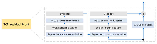
Figure 2.
TCN residual block structure.
Although the TCN model has demonstrated significant advantages in processing long-term time series, its unidirectional dependency limits the integration of bidirectional information. Therefore, this paper employs a bidirectional TCN architecture (BiTCN), whose structure is shown in Figure 3. The core structure of BiTCN consists of forward and backward branches. The forward branch employs TCN residual blocks to process raw time series, capturing multi-scale local features of the original temporal data. The backward branch reverses the input sequence via a flipping layer, then utilizes TCN residual blocks to extract complementary information from the opposite temporal direction. By combining bidirectional feature fusion with causality constraints, the architecture effectively enhances the model’s comprehensive extraction and expression capabilities for temporal features while preserving parallel computing power.
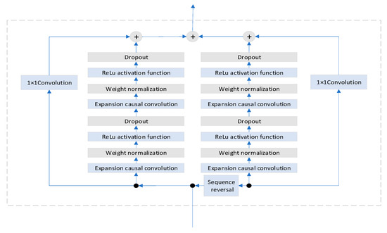
Figure 3.
BiTCN residual block structure.
2.2. Bidirectional Gated Recurrent Units
GRU represent a specialized RNN architecture designed to address the gradient vanishing or gradient explosion issues that commonly arise in traditional RNNs when processing long sequence data. By introducing a gating mechanism to control information flow, GRUs effectively capture long-term dependencies within sequential data. The core structure of a GRU is the unit, as shown in Figure 4. Each unit contains two gates—a reset gate and an update gate—along with a unit state. The unit state is a critical component of the GRU, persisting throughout the network to store long-term information. The gates regulate the flow of information into the unit state, enabling information retention, updating, and output [28].
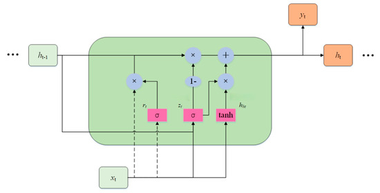
Figure 4.
GRU unit structure.
The reset gate’s(rt) function is to reset the current information and the state information of the hidden layer from the previous moment. The reset gate is computed as follows:
while Wxr and Whr represent the weighting parameters, br represents the bias parameter.
The update gate’s(zt) function is to update the current input information and the state information of the hidden layer from the previous time step. The update gate is computed as follows:
while Wzr and Whc represent the weighting parameters, bz represents the bias parameter.
The formula for calculating the candidate state hht at the current moment is as follows:
while Wxh and Whh represent the weighting parameters, bh represents the bias parameter.
The reset gate rt employs the sigmoid activation function, yielding values between (0, 1). Multiplying rt by the previous hidden layer state ht−1 controls its influence on the current hidden layer state.
The calculation formula for the hidden layer state ht at the current time step is as follows:
zt employs the Sigmoid activation function, yielding values between (0, 1). When zt ≈ 0, the hidden layer state from the previous time step cannot influence the current hidden layer state; when zt ≈ 1, the candidate hidden layer state at the current time step cannot influence the actual hidden layer state at that time.
Bidirectional Gated Recurrent Unit (BiGRU) is an extension of the GRU designed to capture richer contextual information by processing sequence data in both directions. As shown in Figure 5, BiGRU consists of two GRUs running in parallel: a forward GRU and a backward GRU. The forward GRU processes input data in the natural sequence of the time series, while the backward GRU processes the same input data in reverse order. This bidirectional structure enables the model to simultaneously utilize past and future information at each time step, thereby gaining a more comprehensive understanding of the sequence’s context [29].
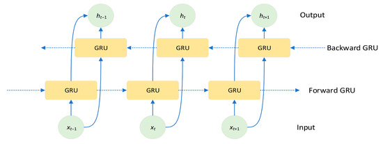
Figure 5.
BiGRU structure.
2.3. Self-Attention Mechanism
Self-Attention Mechanism (SA) is a core algorithm that captures global contextual information by dynamically computing the weight of correlations between elements within a sequence. Its fundamental principle enables the model to adaptively focus on the most relevant information from different positions in the input sequence based on the content at the current processing position, thereby effectively capturing long-range dependencies. The structure of the self-attention mechanism is illustrated in Figure 6.
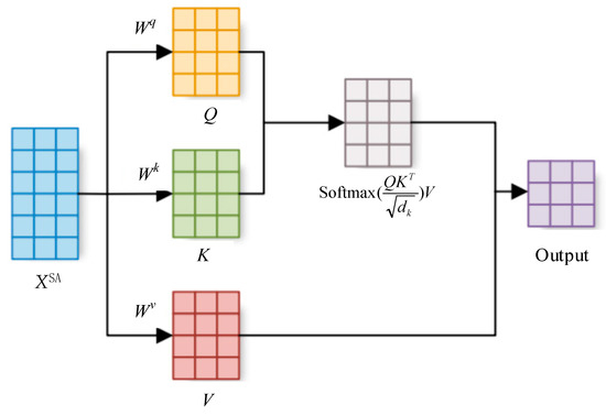
Figure 6.
Self-attention mechanism structure.
The computational process of the self-attention mechanism involves the following steps:
Step 1: Generate query, key, and value vectors. Given the input sequence XSA = [x1, x2,…, xn], generate the query vector Q, key vector K, and value vector V through three linear transformations:
while Wq, Wk, and Wv are trainable weight matrices that map the input to the query, key, and value spaces, respectively.
Step 2: Calculate the attention score. The attention score is computed by taking the dot product of the query vector and the key vector:
To prevent the dot product result from becoming excessively large and causing the gradient to vanish, it is typically divided by a scaling factor , where dk is the dimension of the key vector:
Step 3: Compute the attention outputs. Normalize the attention scores using the Softmax function to obtain attention weights. Then, perform a weighted sum over the value vector using these attention weights to generate the final output [30]:
2.4. Improved Whale Optimization Algorithm
Whale Optimization Algorithm (WOA) is a novel metaheuristic optimization algorithm proposed by Australian scholars Mirjalili and Lewis in 2016 [31]. This algorithm is inspired by the unique hunting behavior of humpback whales—the bubble net hunting method. To enhance the performance of the White-Ocean Algorithm (WOA) in tackling complex optimization problems characterized by high dimensions, multiple peaks, and non-convexity, this paper introduces a dynamic dual mutation mechanism based on the traditional WOA. The specific optimization steps of the IWOA are as follows:
Step 1 Within the domain of the production variables defined by the constraints of the optimization model, randomly generate a set of positions for whale individuals.
Step 2 Set the population size N, maximum iteration count Tmax, and convergence constant a.
Step 3 Evaluate the fitness of each individual based on the objective function of the model. For each whale individual, compute its objective function value.
Step 4 Generate constraints for each whale individual using the penalty function method based on the optimization model’s constraints. The degree of constraint violation is added to the objective function as a penalty term. The penalty term is the product of the penalty coefficient and the sum of all constraint violations for the individual, as shown in the following equation.
while denotes the fitness function of an individual , p represents a large penalty coefficient, and Vi indicates the number of violations of constraints by the individual .
Step 5 Update each individual’s position based on the dynamic double-mutation whale optimization algorithm’s prey-enveloping, bubble-net attack, and random search mechanisms.
The calculation formula for the encirclement hunting mechanism is as follows:
while represents the position vector of the current optimal solution, denotes the position vector of the current individual, and and are coefficient vectors. The calculation is as follows:
In this process, linear decrease from 2 to 0 occurs during iteration, while is a random vector within the range [0, 1].
The calculation formula for the bubble attack mechanism is as follows:
where represents the distance between the whale and its prey, b is the constant defining the logarithmic spiral shape, and l is a random number within the range [−1, 1].
Step 6 implements a dynamic double mutation mechanism, where in each iteration cycle, a portion of individuals are selected based on dynamic strategy to undergo Cauchy and Gaussian mutations, thereby injecting new diversity.
Cauchy mutation leverages the long-tail characteristics of the Cauchy distribution to introduce significant perturbations, helping individuals escape local optima and enhance global exploration. Gaussian mutation leverages the concentrated nature of the Gaussian distribution to perform small, precise searches, enhancing local exploration capabilities. Dynamic selection measures diversity by calculating the current average distance or similarity within the population. When diversity is too low (indicating a local optimum), the probability of applying Cauchy mutation increases; when diversity is high, the probability of applying Gaussian mutation increases to facilitate fine-grained searches.
The formula for calculating the Cauchy mutation is as follows:
while Cauchy(0,1) represents random numbers generated by the standard Cauchy distribution, η is the mutation step size control parameter, and denotes the current optimal solution.
The formula for Gaussian mutation is as follows:
while Gaussian(0,1) generates random numbers from the standard Gaussian distribution.
The probability Pc of selecting a Cauchy mutation and the probability Pg of selecting a Gaussian mutation are calculated using the following dynamic selection mechanism formula:
where Dcurrent is the current population diversity measure, Dmax is the maximum value of population diversity, and Pmin and Pmax are the minimum and maximum values of probability.
The formula for calculating population diversity D is as follows:
where N is the population size, L is the diagonal length of the search space, d is the problem dimension, is the value of the j dimension for the i individual, and is the population mean for the j dimension.
Step 7 The optimization algorithm terminates when the maximum iteration count Tmax is reached or when the solution quality converges after consecutive iterations.
2.5. IWOA-BiTCN-BiGRU-SA Framework
The proposed IWOA-BiTCN-BiGRU-SA forecasting framework primarily consists of the bidirectional Temporal Convolutional Networks, bidirectional Gated Recurrent Networks, self-attention mechanism, and improved whale optimization algorithm mentioned in this chapter. This model employs BiTCN to capture long-term sequence dependencies, utilizes BiGRU to learn sequence information from both forward and backward directions, and leverages IWOA for automatic hyperparameter optimization. The mean squared error between predicted and actual values serves as the fitness function for IWOA, evaluating the performance of BiTCN-BiGRU models with varying hyperparameter configurations, as illustrated below:
where and represent the actual value and predicted value, respectively, and m denotes the number of samples in the training set.
The workflow of the IWOA-BiTCN-BiGRU-SA prediction framework is shown in Figure 7.
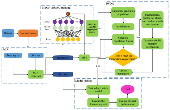
Figure 7.
IWOA-BiTCN-BiGRU-SA framework.
The specific workflow of the IWOA-BiTCN-BiGRU-SA framework is as follows:
Step 1: Preprocess and normalize the original dataset to ensure all feature data and target prediction data share the same proportional scale. Step 2: Divide the processed dataset into training and testing sets. Step 3: Calculate the feature contribution rate and cumulative contribution rate to determine the required feature dimension k. Apply Principal Component Analysis(PCA) to reduce the original feature dimension to k, thereby generating new training and testing sets. Step 4: Build the BiTCN-BiGRU model based on the BiGRU architecture integrated with the BiTCN module. The BiTCN model effectively extracts latent information from time-series data. BiGRU efficiently processes large-scale sequence data, feeding the feature information collected by BiTCN into the BiGRU layer for load forecasting. During training, backpropagation jointly optimizes parameters across both modules, enabling end-to-end learning. Step 5: The BiTCN-BiGRU model is trained using the training dataset and IWOA. After multiple iterations, the optimal hyperparameters for the BiTCN-BiGRU model are calculated. Step 6: The BiTCN-BiGRU model is configured using the optimal hyperparameters from Step 5. The model is validated using the test dataset, and its performance is evaluated by comparing predictions with the target data.
The innovation of the proposed IWOA-BiTCN-BiGRU-SA framework is primarily reflected in the following aspects:
Synergistic Bidirectional Architecture: Unlike models that utilize unidirectional TCN or a simple cascade of TCN and RNN, this framework pioneers a Bidirectional TCN coupled with a Bidirectional GRU. This design enables a two-stage, comprehensive extraction of temporal features. The BiTCN layer first performs a coarse-grained capture of multi-scale local patterns from both past and future contexts. Subsequently, the BiGRU layer conducts a fine-grained modeling of the long-term, bidirectional dependencies within these refined features. This synergistic bidirectional co-optimization across different granularities allows the model to form a more holistic understanding of the load sequence, effectively overcoming the limitations of single-directional models in capturing complex temporal dynamics.
Adaptive Feature Refinement via Self-Attention: The incorporation of the Self-Attention (SA) mechanism after the BiGRU layer introduces a powerful adaptive weighting capability. It dynamically identifies and assigns higher weights to the most critical time steps and feature representations from the BiGRU outputs. This process enhances the model’s focus on pivotal load fluctuation periods (e.g., peak demand), thereby improving not only the prediction accuracy but also the model’s robustness and interpretability.
End-to-End Hyperparameter Optimization with IWOA: Replacing manual trial-and-error and conventional optimization algorithms, the Improved Whale Optimization Algorithm (IWOA) is employed for end-to-end automatic hyperparameter tuning. The introduced dynamic dual-mutation mechanism (Cauchy and Gaussian) equips the IWOA with a superior ability to escape local optima and conduct a more efficient global search. This ensures that the complex hybrid deep learning model can consistently converge to a high-performance configuration, significantly boosting generalization ability and training stability.
In summary, the innovation of this framework lies not merely in the combination of advanced components, but in their deep integration and organic synergy. It establishes a cohesive pipeline where BiTCN and BiGRU collaboratively perform bidirectional feature learning, the SA mechanism adaptively refines these features, and the IWOA robustly optimizes the entire architecture. This integrated approach successfully addresses the key challenges in CAC load forecasting, leading to a substantial performance improvement.
3. Experiments and Discussion
3.1. Datasets Introduction
The experimental data utilized in this work was obtained from the open dataset of the “TIPDM Cup” Data Analysis Professional Skills Competition [32]. This collection originates from the central air conditioning system of a large tropical building, which has a height of 20.3 m and a total floor space of 25,000 square meters, with air-conditioned areas covering 19,000 square meters. The dataset covers the period from 4 October to 29 December 2016, with data recorded at one-minute intervals. It includes 88,840 hourly load entries and natural environmental factors affecting cooling electricity demand. During this period, continuous cooling was required for this large office building. For modeling purposes, the dataset was partitioned into an 80% training set and a 20% test set [33]. The simulations were performed using Python 3.7, together with the PyTorch 1.5.0 framework and the scikit-learn library 1.0.2, on a PC equipped with an Intel 11th Gen i5 processor and 16 GB of RAM. The detailed composition of the dataset is provided in Table 1.

Table 1.
The contents of the dataset [33].
3.2. Input Feature Dimension Reduction
In this study, the target variable is the total system load (loadays) as shown in Table 1, while the input features for the model comprise the other nine data items. However, data with as many as nine dimensions proves overly complex for training, increasing both the difficulty of model training and the risk of overfitting. To mitigate the curse of dimensionality, the PCA algorithm is employed to reduce the dimensionality of the feature data, thereby enhancing the training efficiency and accuracy of the subsequent model.
Figure 8 shows the cumulative variance contribution rate of the feature matrix at different retained dimensions. Retaining the first five feature dimensions simultaneously minimizes information loss and reduces data dimensionality. Figure 9a displays the correlations between normalized original feature data. This figure reveals strong correlations among wind speed data at different heights, with similar correlations also present in wind direction data across varying altitudes. Conversely, no correlation exists between wind speed and wind direction data. Thus, redundancy exists among these feature data, concealing overlapping information. This not only leads to high computational complexity and the curse of dimensionality but also often causes model overfitting due to fitting too many features. Figure 9b displays the correlation matrix among the five new feature groups after dimensionality reduction. It can be observed that no correlations remain among the new feature data. They now possess independent information and eliminate the redundancy present in the original data.
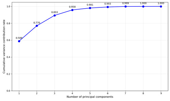
Figure 8.
Amount of variance explained by PCA.
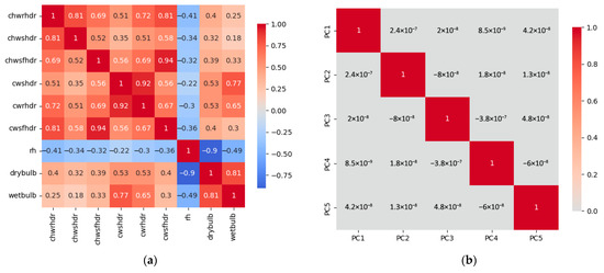
Figure 9.
Amount of variance explained by PCA: (a) Before reduction; (b) After reduction.
3.3. Performance Criteria
To evaluate the accuracy of the IWOA-BiTCN-BiGRU-SA prediction framework, three error metrics were employed as assessment criteria: Mean Absolute Error (MAE), Root Mean Square Error (RMSE), and Coefficient of Determination (R2). The calculation formulas are as follows:
3.4. Comparative Experiment
To validate the effectiveness of the proposed IWOA-BiTCN-BiGRU-SA framework for air conditioning load forecasting, the framework was tested on a dataset subjected to dimensionality reduction. Table 2 presents the experimental parameters of the IWOA-BiTCN-BiGRU-SA framework. Notably, the hyperparameters for BiTCN and BiGRU are specified within a range, with the IWOA identifying the optimal values. Furthermore, this subsection conducts comparative experiments against regression models including LSTM, GRU, RNN, CNN, and SVM based on the performance criteria proposed in Section 3.3, demonstrating the framework’s superiority.
Table 2.
Parameter of the IWOA-BiTCN-BiGRU-SA framework.
Table 3 shows the predictive performance of the aforementioned models on the dataset. Compared to the traditional machine learning model SVM, the proposed IWOA-BiTCN-BiGRU-SA framework demonstrates a significant advantage in prediction accuracy. Compared to the traditional SVM model, this framework reduces the MAE and RMSE metrics by 60.01% and 56.66%, respectively. Moreover, this framework also demonstrates strong superiority over individual deep learning models (CNN, RNN, GRU, LSTM). Its MAE is reduced by 58.10%, 56.64%, 56.44%, and 56.43% compared to other deep learning models, respectively. The framework’s RMSE was reduced by 58.28%, 52.28%, 51.84%, and 52.10% compared to other deep learning models. This is because the BiTCN module in the IWOA-BiTCN-BiGRU-SA framework can flexibly control the model’s coverage of historical information by adjusting the number of layers, expansion rate, and convolution kernel size, thereby enhancing its ability to extract sequence features. Moreover, the BiGRU module extracts bidirectional information concealed within time series data. Furthermore, the SA mechanism captures internal sequence correlations through dynamic weight allocation, improving training efficiency. The IWOA enhances the model’s applicability for air conditioning load forecasting by optimizing hyperparameters. Consequently, the synergistic interaction among modules within the IWOA-BiTCN-BiGRU-SA framework substantially elevates its predictive capability.
Table 3.
Comparison results between the proposed model and other predictive models.
3.5. Ablation Experiment
To evaluate the contribution of each module within the WOA-BiTCN-BiGRU-SA framework to its predictive performance, this section conducts an ablation study. The framework is compared against BiTCN, BiGRU, BiTCN-SA, BiGRU-SA, TCN-BiGRU, BiTCN-BiGRU, and BiTCN-BiGRU-SA using the same dataset. Data from 168 sample points in the test dataset will be used to demonstrate the predictive performance of each model, as illustrated in Figure 10 and Figure 11.
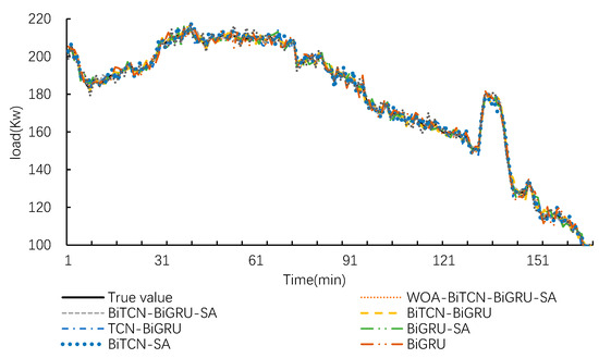
Figure 10.
Prediction curves of the test set for various models.
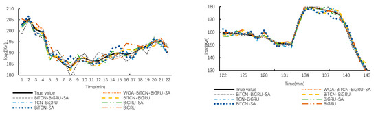
Figure 11.
Prediction results at local time points.
Figure 10 displays the comparison curves between the predicted load values and actual load values for each model on the test set. Overall, the prediction curves of all models capture the actual load variation curves, though significant differences exist at peaks and troughs. Figure 11 provides an enlarged view of the curves to further evaluate the models’ predictive capabilities at granular levels. It is evident that the IWOA-BiTCN-BiGRU-SA framework’s prediction curve aligns more closely with the actual load curve. Although some other models exhibit closer predictions to actual values at specific points in time, their overall predictive performance still demonstrates substantial deviation.
Table 4 shows the performance of various models in central air conditioning load forecasting based on performance criteria. It can be seen that the models exhibit varying performance in the air conditioning load forecasting task.
Table 4.
Comparison of prediction performance of all models.
Comparing BiTCN-BiGRU and TCN-BiGRU reveals that BiTCN enhances the model’s prediction accuracy relative to standard TCN. The RMSE of TCN-BiGRU is 10.8211 kW, while that of BiTCN-BiGRU is 9.6564 kW. This indicates that BiTCN can more effectively capture the bidirectional dependencies in time-series data compared to TCN, thereby enhancing the accuracy of load forecasting.
Comparing BiTCN-BiGRU-SA with BiTCN-BiGRU reveals that introducing the self-attention (SA) mechanism further improves model performance. BiTCN-BiGRU-SA reduces RMSE by 0.5352 kW, decreases MAE by 5.64%, and increases R2 by 0.55%. This indicates that the SA mechanism enhances the model’s focus on critical time steps, improves feature extraction capabilities, and further reduces prediction errors.
Comparing IWOA-BiTCN-BiGRU-SA with BiTCN-BiGRU-SA, it is evident that applying IWOA for hyperparameter optimization significantly improves the model’s prediction accuracy. The RMSE of IWOA-BiTCN-BiGRU-SA decreased by kW, the MAE decreased by 1.2513 kW, and the R2 increased by 0.19%. This result indicates that IWOA can effectively search for the optimal hyperparameter combination, enabling the model to achieve superior prediction performance.
The proposed IWOA-BiTCN-BiGRU-SA model demonstrated the best performance in central air conditioning load forecasting. It outperformed other comparison models in RMSE, MAE, and R2 metrics, significantly reducing prediction errors while enhancing the model’s ability to capture load variations.
4. Conclusions
This study proposes a novel hybrid load forecasting model for central air conditioning systems, termed IWOA-BiTCN-BiGRU-SA, which integrates an Improved Whale Optimization Algorithm (IWOA) with a deep learning architecture composed of Bidirectional Temporal Convolutional Networks (BiTCN), Bidirectional Gated Recurrent Units (BiGRU), and a Self-Attention mechanism (SA). The model’s performance was rigorously validated through comparative and ablation experiments on a real-world operational dataset. The conclusions of this study are as follows.
- The application of the Improved Whale Optimization Algorithm (IWOA) for hyperparameter optimization proved highly effective. The IWOA-optimized model achieved an RMSE of 7.8699 kW, which is 1.2513 kW lower than the same model without IWOA optimization. This demonstrates that IWOA can automatically identify the optimal hyperparameter combination, significantly enhancing the model’s prediction accuracy and stability compared to manual tuning.
- The hybrid BiTCN-BiGRU architecture demonstrated superior capability in extracting complex temporal features. Compared to the standard TCN-BiGRU model, the BiTCN-BiGRU model reduced the RMSE by 1.1647 kW. This confirms that the bidirectional structure of BiTCN can more effectively capture multi-scale temporal dependencies from both past and future contexts, leading to a more comprehensive feature representation than a unidirectional TCN.
- The introduction of the self-attention (SA) mechanism further improved the model’s performance. The BiTCN-BiGRU-SA model reduced the RMSE by 0.5352 kW compared to the BiTCN-BiGRU model. This indicates that the SA mechanism successfully enhances the model’s ability to adaptively focus on critical time steps and features, thereby improving the robustness and interpretability of the predictions.
- Comprehensive comparisons with benchmark models demonstrate the overall superiority of the proposed framework. The IWOA-BiTCN-BiGRU-SA model achieved reductions in RMSE of 8.5568 kW, 8.4728 kW, and 10.2872 kW compared to standalone LSTM, GRU, and SVM models, respectively. These results highlight the significant synergistic effect achieved by integrating the respective advantages of IWOA, BiTCN, BiGRU, and SA into a unified framework.
In summary, the IWOA-BiTCN-BiGRU-SA prediction model exhibits high accuracy and strong robustness, providing a reliable data-driven solution for the short-term load forecasting of central air conditioning systems. This offers effective technical support for intelligent energy management and operational optimization in large buildings. In the future, we will explore the application of this framework to load forecasting for integrated energy systems and other types of buildings to further verify its generalization capability.
Author Contributions
Conceptualization, Y.X.; methodology, Y.X.; software, R.H. and W.H.; validation, Y.X. and Y.L.; formal analysis, Y.X.; investigation, Y.X., Y.L. and C.Z.; resources, R.H., W.H. and C.L.; data curation, Y.L. and C.Z.; writing—original draft preparation, Y.X.; writing—review and editing, C.L.; visualization, Y.X.; supervision, R.H., W.H. and C.L.; project administration, R.H., W.H. and C.L.; funding acquisition, R.H. and W.H. All authors have read and agreed to the published version of the manuscript.
Funding
This study is funded by China Yangtze Power Co., Ltd. Research and Application Demonstration Project on Energy-saving Operation and Carbon Management Technologies for Data Centers (Z342302012).
Institutional Review Board Statement
Not applicable.
Informed Consent Statement
Not applicable.
Data Availability Statement
The original contributions presented in this study are included in the article. Further inquiries can be directed to the corresponding author.
Conflicts of Interest
Authors Wei He and Rui Hua were employed by the companies China Yangtze Power Co., Ltd. and Three Gorges Electric Energy Co., Ltd. Authors Yuce Liu and Chaohui Zhou were employed by the company China Three Gorges Corporation. The remaining authors declare that the research was conducted in the absence of any commercial or financial relationships that could be construed as a potential conflict of interest. The authors declare that this study received funding from China Yangtze Power Co., Ltd. Authors Wei He and Rui Hua are employed by the company. Furthermore, author Chaoshun Li served as the principal investigator for this project and received funding from China Yangtze Power Co., Ltd.
Abbreviations
The following abbreviations are used in this manuscript:
| CAC | Accurate load forecasting of central air conditioning |
| IWOA | Improved Whale Optimization Algorithm |
| BiTCN | Bidirectional Temporal Convolutional Networks |
| BiGRU | Bidirectional Gated Recurrent Units |
| SA | Self-attention |
| RSME | Root mean square error |
| PCA | Principal component analysis |
| CEHT | Incorporating the cumulative effect of high temperature |
| PB-MLR | Physical-Based Multiple Linear Regression |
| SVM | Support Vector Machines |
| ANN | Artificial Neural Networks |
| GBDT | Gradient-Boosted Decision Tree |
| CNN | Convolutional Neural Networks |
| LSTM | Long Short-Term Memory |
| WTD | Wavelet Threshold Denoising |
| GNN | Graph Neural Networks |
| GA | Genetic Algorithm |
| PSO | Particle Swarm Optimization |
| GWO | Grey Wolf Optimization |
| SSA | Sparrow Search Algorithm |
| IVMD | Improved Variational Mode Decomposition |
| LSSVM | Least Squares Support Vector Machine |
| RS | Rough Set |
| DELM | Deep Extreme Learning Machine |
| TCNs | Temporal Convolutional Networks |
| MAE | Mean Absolute Error |
| RMSE | Root Mean Square Error |
| R2 | Coefficient of Determination |
References
- China will Formulate an Action Plan This Year to Achieve Peak Carbon Emissions Before 2030. Available online: https://www.gov.cn/zhengce/2021-03/06/content_5590830.htm (accessed on 28 September 2025).
- Cai, M.; Pipattanasomporn, M.; Rahman, S. Day-ahead building-level load forecasts using deep learning vs. traditional time-series techniques. Appl. Energy 2019, 236, 1078–1088. [Google Scholar] [CrossRef]
- Pallonetto, F.; Jin, C.; Mangina, E. Forecast electricity demand in commercial building with machine learning models to enable demand response programs. Energy AI 2022, 7, 100121. [Google Scholar] [CrossRef]
- Li, W.; Gong, G.; Ren, Z.; Ouyang, Q.; Peng, P.; Chun, L.; Fang, X. A method for energy consumption optimization of air conditioning n load prediction and energy flexibility. Energy 2022, 243, 123111. [Google Scholar] [CrossRef]
- Ma, X.; Chen, F.; Wang, Z.; Li, K.; Tian, C. Digital twin model for chiller fault diagnosis based on SSAE and transfer learning. Build. Environ. 2023, 243, 110718. [Google Scholar] [CrossRef]
- Qiao, Q.; Yunusa-Kaltungo, A.; Edwards, R.E. Towards developing a systematic knowledge trend for building energy consumption prediction. J. Build. Eng. 2021, 35, 101967. [Google Scholar] [CrossRef]
- Eid, E.; Foster, A.; Alvarez, G.; Ndoye, F.-T.; Leducq, D.; Evans, J. Modelling energy consumption in a Paris supermarket to reduce energy use and greenhouse gas emissions using EnergyPlus. Int. J. Refrig. 2024, 168, 1–8. [Google Scholar] [CrossRef]
- Yu, K.; Cao, Z.; Liu, Y. Research on the optimization control of the central air-conditioning system in university classroom buildings based on TRNSYS software. Procedia Eng. 2017, 205, 1564–1569. [Google Scholar] [CrossRef]
- Olu-Ajayi, R.; Alaka, H.; Sulaimon, I.; Sunmola, F.; Ajayi, S. Building energy consumption prediction for residential buildings using deep learning and other machine learning techniques. J. Build. Eng. 2022, 45, 103406. [Google Scholar] [CrossRef]
- Vats, U.; Roga, S.; Sinha, A.; Singh, A.K.; Dharua, S.S.; Shah, H. Design and Performance Analysis of Heating, Cooling and Air Quality in a Sustainable Building using eQUEST. In Proceedings of the 2022 1st International Conference on Sustainable Technology for Power and Energy Systems (STPES), New York, NY, USA, 4–6 July 2022; pp. 1–5. [Google Scholar]
- Qiang, G.; Zhe, T.; Yan, D.; Neng, Z. An improved office building cooling load prediction model based on multivariable linear regression. Energy Build. 2015, 107, 445–455. [Google Scholar] [CrossRef]
- Chen, S.; Zhou, X.; Zhou, G.; Fan, C.; Ding, P.; Chen, Q. An online physical-based multiple linear regression model for building’s hourly cooling load prediction. Energy Build. 2022, 254, 111574. [Google Scholar] [CrossRef]
- Dahl, M.; Brun, A.; Andresen, B.G. Using ensemble weather predictions in district heating operation and load forecasting. Appl. Energy 2017, 193, 455–465. [Google Scholar] [CrossRef]
- Fan, C.; Ding, Y. Cooling load prediction and optimal operation of HVAC systems using a multiple nonlinear regression model. Energy Build. 2019, 197, 7–17. [Google Scholar] [CrossRef]
- Yun, K.; Luck, R.; Mago, J.P.; Cho, H. Building hourly thermal load prediction using an indexed ARX model. Energy Build. 2012, 54, 225–233. [Google Scholar] [CrossRef]
- Li, Q.; Meng, Q.; Cai, J.; Yoshino, H.; Mochida, A. Applying support vector machine to predict hourly cooling load in the building. Appl. Energy 2008, 86, 2249–2256. [Google Scholar] [CrossRef]
- Deb, C.; Eang, S.L.; Yang, J.; Santamouris, M. Forecasting diurnal cooling energy load for institutional buildings using Artificial Neural Networks. Energy Build. 2016, 121, 284–297. [Google Scholar] [CrossRef]
- Yanxiao, F.; Qiuhua, D.; Xi, C.; Yakkali, S.S.; Wang, J. Space cooling energy usage prediction based on utility data for residential buildings using machine learning methods. Appl. Energy 2021, 291, 116814. [Google Scholar] [CrossRef]
- Zhang, W.; Yu, J.; Zhao, A.; Zhou, X. Predictive model of cooling load for ice storage airconditioning system by using GBDT. Energy Rep. 2021, 7, 1588–1597. [Google Scholar] [CrossRef]
- Zhao, R.; Wei, D.; Ran, Y.; Zhou, G.; Jia, Y.; Zhu, S.; He, Y. Building Cooling load prediction based on LightGBM. IFAC Pap. 2022, 55, 114–119. [Google Scholar] [CrossRef]
- Wang, Z.; Hong, T.; Piette, A.M. Building thermal load prediction through shallow machine learning and deep learning. Appl. Energy 2020, 263, 114683. [Google Scholar] [CrossRef]
- Wang, F.; Cen, J.; Yu, Z.; Deng, S.; Zhang, G. Research on a hybrid model for cooling load prediction based on wavelet threshold denoising and deep learning: A study in China. Energy Rep. 2022, 8, 10950–10962. [Google Scholar] [CrossRef]
- Zhao, A.; Zhang, Y.; Zhang, Y.; Yang, H.; Zhang, Y. Prediction of functional zones cooling load for shopping mall using dual attention based LSTM: A case study. Int. J. Refrig. 2022, 144, 211–221. [Google Scholar] [CrossRef]
- Zou, M.; Huang, W.; Jin, J.; Hu, B.; Liu, Z. Deep spatio-temporal feature fusion learning for multistep building cooling load forecasting. Energy Build. 2024, 322, 114735. [Google Scholar] [CrossRef]
- Zhou, M.; Yu, J.; Wang, M.; Quan, W.; Bian, C. Research on the combined forecasting model of cooling load based on IVMD-WOA-LSSVM. Energy Build. 2024, 317, 114339. [Google Scholar] [CrossRef]
- Lei, L.; Shao, S. Prediction model of the large commercial building cooling loads based on rough set and deep extreme learning machine. J. Build. Eng. 2023, 80, 107958. [Google Scholar] [CrossRef]
- Bai, S.; Kolter, J.Z.; Koltun, V. An empirical evaluation of generic convolutional and recurrent networks for sequence modeling. arXiv 2018, arXiv:1803.01271. [Google Scholar] [CrossRef]
- Xiao, Y.; Zou, C.; Chi, H.; Fang, R. Boosted GRU model for short-term forecasting of wind power with feature-weighted principal component analysis. Energy 2023, 267, 126503. [Google Scholar] [CrossRef]
- Yang, X.; Peng, S.; Zhang, Z.; Du, Y.; Linghu, L. Thermal error prediction in dry hobbing machine tools: A CNN-BiGRU network with spatiotemporal feature fusion. Measurement 2025, 256, 118389. [Google Scholar] [CrossRef]
- Chen, W.; Huang, H.; Ma, X. The short-term wind power prediction based on a multi-layer stacked model of BOsingle bondCNN-BiGRU-SA. Digit. Signal Process. 2025, 156, 104838. [Google Scholar] [CrossRef]
- Mirjalili, S.; Lewis, A. The Whale Optimization Algorithm. Adv. Eng. Softw. 2016, 95, 51–67. [Google Scholar] [CrossRef]
- The 5th TipDM Cup Data Analysis Professional Skills Competition. Available online: https://www.tipdm.org (accessed on 28 September 2025).
- Guo, Y.; Chen, M.; Wang, H.; Chu, P.; Sheng, Y.; Li, H. Hybrid forecasting model for central air conditioning load based on CEEMDAN and WTCN-GRU. Int. J. Refrig. 2025, 176, 373–385. [Google Scholar] [CrossRef]


Disclaimer/Publisher’s Note: The statements, opinions and data contained in all publications are solely those of the individual author(s) and contributor(s) and not of MDPI and/or the editor(s). MDPI and/or the editor(s) disclaim responsibility for any injury to people or property resulting from any ideas, methods, instructions or products referred to in the content. |
© 2025 by the authors. Licensee MDPI, Basel, Switzerland. This article is an open access article distributed under the terms and conditions of the Creative Commons Attribution (CC BY) license (https://creativecommons.org/licenses/by/4.0/).