AutoML-Assisted Classification of Li-Ion Cell Chemistries from Cycle Life Data: A Scalable Framework for Second-Life Sorting

Abstract

Repurposing lithium-ion (Li-ion) batteries for second-life applications, such as stationary energy storage, offers significant economic and environmental benefits as these cells reach the end of their initial service life. Accurate and scalable classification of used Li-ion cell chemistries is essential for efficient sorting and safe repurposing, especially when manufacturer metadata is unavailable. This study presents a robust, automated machine learning (AutoML) framework, implemented in MATLAB R2024b and its toolboxes, for classifying three commercial 18,650 cell chemistries (LFP, NMC, and NCA) using long-term cycle life data. The workflow integrates structured data ingestion, segmentation, and multi-tiered feature engineering, extracting over 75 diagnostic features per cycle, including statistical, cumulative, segment-specific, and differential curve metrics. Feature selection is performed using principal component analysis and sequential forward selection, while Bayesian optimisation within AutoML identifies the optimal classification model. The resulting K-Nearest Neighbours classifier achieves over 99% test accuracy, demonstrating the effectiveness of the approach. This framework enables research-grade, metadata-independent classification and provides a scalable foundation for future industrial battery sorting and second-life applications.

1. Introduction

The use of lithium-ion (Li-ion) batteries in electric vehicles (EVs), consumer electronics, power tools, medical devices, marine applications, and energy storage systems is increasing as the world moves toward using more electricity from renewable energy sources [1]. As batteries reach the end of their first service life, tracking the growing volume of used cells becomes increasingly important. Recovering valuable materials like lithium, cobalt, aluminium, manganese and nickel can be achieved through recycling, but it is often not profitable and requires a lot of energy [2]. Therefore, using aged batteries for second-life applications, such as stationary energy storage, is better for the environment and cost-effective because it makes them last longer until they are recycled [3].

An accurate classification of Li-ion battery cell chemistry and condition is essential for the reliable operation of second-life applications. Common chemistries include Lithium Iron Phosphate (LFP), Nickel Manganese Cobalt Oxide (NMC), and Nickel Cobalt Aluminium Oxide (NCA), each with distinct electrochemical properties and degradation pathways [4]. Misclassification can lead to performance issues, system incompatibility, and safety risks. Traditional methods, such as visual inspection and electrochemical impedance spectroscopy, are often unreliable or impractical for large-scale use, particularly when manufacturer metadata is missing [5]. This challenge is especially relevant in research, diagnostic, and second-life sorting contexts, where reliable classification of Li-ion battery chemistries is critical to enabling scalable sorting frameworks [6].

A few researchers have looked into using data-driven methods to solve the aforementioned problems. Thompson et al. [7] developed DiffCapAnalyzer, a Python package for constructing and analysing differential or Incremental Capacity (dQ/dV) Analysis (ICA) curves. This tool helped them to extract electrochemical descriptors from differential capacity curves that are important for identifying cell chemistries. Their method was able to differentiate LiCoO₂ and LiFePO₄ with 77% accuracy in a classification task using a support vector machine. According to Neubauer et al. [8], the main obstacles to second-life adoption are the deficiency of standard classification protocols and the high cost of manual testing. Lucaferri et al. [9] categorised battery modelling and classification strategies into three groups: voltage-based, impedance-based, and data-driven. They noted that data-driven approaches are the most flexible but depend heavily on the quality of features and the robustness of the model.

Odinsen et al. [10] suggested using regression models to directly estimate ICA curves from raw cycling data, enabling downstream classification without curve fitting. Amuta et al. [11] proposed a classification method based on temperature that utilises supervised learning, but it necessitates thermal data that is not always obtainable in second-life contexts. Karaoğlu and Ulgut [12] analysed short-term measurements for predicting cell chemistry using decision tree algorithms. Their method achieved 100% classification accuracy on a held-out test set of 55 batteries, demonstrating strong performance within the scope of their dataset. However, due to the simplicity of the model and the limited sample diversity, its generalisability to larger datasets with broader battery chemistries and degradation states remains uncertain. Wett et al. [13] proposed a machine learning technique that utilises synthesised open-circuit voltage (OCV) curves derived from electrochemical modelling, achieving up to 89% accuracy in identifying LFP and NMC chemistry. Although promising, their method is constrained by partial OCV measurements and synthetic data, which limit scalability and accuracy.

Building on these insights, this study proposes a scalable AutoML-based framework that leverages long-term cycle life data for chemistry classification. Unlike visual inspection or impedance-based techniques, which are often impractical for large-scale sorting, the proposed method uses a comprehensive suite of diagnostic metrics extracted from raw cycling data to enable automated, metadata-independent classification.

Despite significant advancements in Automated Machine Learning (AutoML) that have streamlined algorithm selection and hyperparameter optimisation, real-world cell sorting still faces challenges, including the need for robust, scalable, and interpretable solutions. To address these, we employ MATLAB’s AutoML in combination with three diagnostic methods: Incremental Capacity Analysis (ICA), Differential Voltage Analysis (DVA), and Differential Thermal Analysis (DTA). ICA provides valuable insights into cell mechanisms and health via voltage–capacity curves, while DVA and DTA extract high-resolution electrochemical and thermal features from cycling data. AutoML then facilitates optimal model selection and tuning without requiring expert intervention.

The framework incorporates a multi-tiered feature extraction strategy using MATLAB’s Predictive Maintenance Toolbox™ (PMT), generating over 75 features per cycle. These include statistical descriptors, cumulative metrics, segment-specific indicators, and differential curve features (see Section 4.2). By computing these features for each charge step and cycle, the framework enables detailed tracking of battery behaviour across chemistries and over time. Unlike prior studies [7,12,13] that rely on a limited set of manually selected models, or experimentally driven studies [14], our approach makes use of experimental data and automates both feature generation and selection, making it suitable for scalable workflows that can later be leveraged for industry-level cell sorting. It also shows promise for future adaptation to rapid diagnostic workflows using short-duration measurement data.

This method offers several key advantages: (a) reliable identification of cell chemistries from cycle life data; (b) independence from manufacturer-specific information; and (c) suitability for research-grade classification and second-life battery assessment, even when only partial cycling data is available. By enabling accurate, automated, and scalable classification, the framework supports circular economy models, reduces electrochemical waste, and promotes sustainable battery repurposing [15].

While transfer learning has shown promise in addressing data scarcity and domain variability in battery diagnostics [16], this study does not employ transfer learning methods such as CORAL, domain adversarial networks, or federated learning. Instead, our approach leverages AutoML to automate model selection and hyperparameter tuning, using a rich set of diagnostic features extracted from long-term cycling data. The framework is designed to be scalable and generalisable across chemistries but does not involve cross-domain adaptation or multi-task learning.

2. Methodology

2.1. Overview of the AutoML-Based Framework

As introduced in Section 1, this study presents a scalable AutoML-based framework for classifying Li-ion cell chemistries using long-term cycling data. Figure 1 visualises the end-to-end pipeline, beginning with raw data ingestion and segmentation, followed by multi-tier feature engineering using MATLAB’s PMT. Features are then processed and passed to an AutoML module for automated model selection, hyperparameter tuning, and evaluation. Final classification results are validated using confusion matrix analysis.

2.2. Data Source and Selection

This study uses Li-ion cycling datasets from BatteryArchive.org, derived from long-term experimental work by Sandia National Laboratories. The BatteryArchive platform provides free access to interactive visualisations of these datasets, allowing users to explore cycling trends and summary statistics online. However, access to the underlying raw time-series data files (which are required for detailed analysis and feature extraction) must be requested directly from Sandia National Laboratories and they are not publicly downloadable by default.

In this study, raw datasets for three commercial 18,650-format chemistries (LFP, NMC, and NCA) were obtained with permission and used for all diagnostic and machine learning analyses. Each cell was subjected to controlled ageing protocols until its capacity declined to approximately 80% of its initial value, with periodic Reference Performance Tests (RPTs) to mark the State of Health (SoH).

Measurements taken during cycling include time, current, voltage, temperature, cycle index, and step index, which are valuable inputs for time-series analysis and feature extraction. Detailed electrochemical performance comparisons across chemistries and cycling conditions are provided by the original studies [14,15] and are not repeated here. In line with BatteryArchive’s data usage policy, reference [17] is cited as the source of the datasets used in this article.

The specific time-series CSV files used in this study are:

• SNL_18650_LFP_25C_0-100_0.5-1C_c_timeseries
• SNL_18650_NMC_25C_0-100_0.5-1C_b_timeseries
• SNL_18650_NCA_25C_0-100_0.5-1C_d_timeseries

Each dataset corresponds to cells cycled under standardised conditions: 25 °C ambient temperature, 0–100% depth of discharge (DoD), and 0.5 C–1 C charge/discharge rates, as indicated in the file names. While this article uses single-cell sample data per test condition, Preger et al. [14] report that most test conditions included at least two cells per chemistry to ensure repeatability. Furthermore, their study includes extensive testing across multiple temperatures and charge/discharge rates, which supports the generalisability of the observed degradation behaviours. As there are no known issues with the selected test conditions or the chosen cells, this supports the reproducibility and reliability of the diagnostic trends used in this study. Future work will extend the framework to incorporate diverse operating conditions and validate classification robustness under real-world scenarios.

Visualisation and analysis of these datasets are presented in Section 3. This includes time-series profiling of current, voltage, and temperature across chemistries (Section 3.1); comparison of early- and late-life cycles to highlight ageing effects (Section 3.2); segmentation and analysis of operational phases (Section 3.3); and exclusion of invalid cycles (Section 3.4). These analyses collectively support the classification framework by providing chemistry-specific behavioural insights and ensuring data integrity.

3. Cycle-Level Data Analysis and Segmentation

To support accurate classification of Li-ion cell chemistries, this section begins with a behavioural analysis of raw long-term cycling data, focusing on electrical and thermal characteristics initially. Section 3.1 presents time-series profiles of current, voltage, and temperature to highlight chemistry-specific trends. Section 3.2 compares early- and late-life cycles to illustrate ageing-related shifts in electrochemical behaviour. Section 3.3 examines the operational phases of Cycle 5 to understand the electrochemical characteristics of each chemistry under a cycle life test condition. Visual diagnostics in Section 3.1, Section 3.2 and Section 3.3 were generated using custom MATLAB plotting scripts. Structured segmentation of the entire dataset, along with the exclusion of invalid cycles in Section 3.4, was performed using the batteryTestDataParser function (part of MATLAB’s PMT), which tags each data point with its corresponding cycle and operational steps. This ensures consistency across chemistries and enables downstream feature engineering and extraction, as detailed in Section 4 and Section 5.

3.1. Time-Series Profiles of Cycle Life Across Chemistries

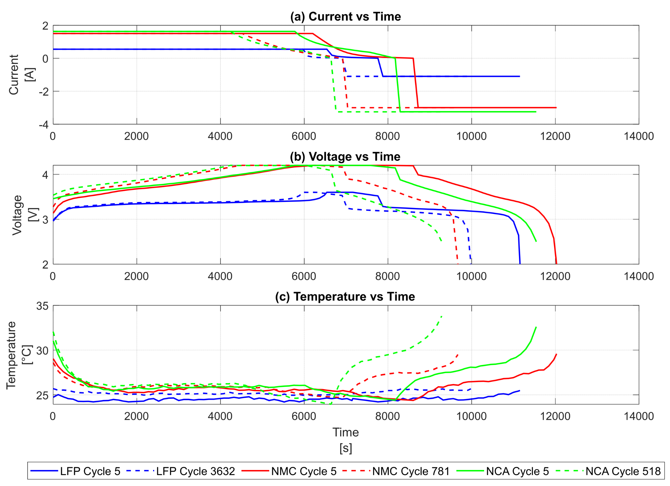
Figure 2 presents time-series profiles of current (Figure 2a), voltage (Figure 2b), and temperature (Figure 2c) for LFP, NMC, and NCA cells, cycled under identical conditions. These profiles exhibit chemistry-specific trends that are distinguishable through detailed analysis and are further supported by the summary of electrical and thermal characteristics in

Table 1. Summary of electrical and thermal characteristics of LFP, NMC, and NCA chemistries, derived from [15] and see Figure 2 for supporting data.

Parameter	LFP	NMC	NCA
Nominal Capacity [Ah]	1.1	3.0	3.2
Current Behaviour	Low magnitude, stable	Fluctuating, high-energy density	Fluctuating, high-energy density
Voltage Behaviour [V]	Narrow, stable (~3.2–3.6)	Broad (~2.5–4.2)	Broad, highest (~2.5–4.2)
Thermal Response	Stable, low heat	Moderate	High, elevated resistance

. Some descriptors in Table 1 are interpretive and excluded from AutoML classification, which operates independently of metadata. These insights support the segmentation and exclusion strategies described later in this section, forming a foundation for robust feature extraction.

In Figure 2, the time-series profiles display distinct electrical and thermal behaviour among the three chemistries, from which key electrical, thermal and very limited electrochemical properties can be inferred. LFP cells have a stable and narrow voltage range with low current magnitudes, which is due to their lower nominal capacity and stable intercalation dynamics. In contrast, NMC and NCA cells exhibit broader voltage ranges and more pronounced current fluctuations, indicative of higher energy densities and complex phase transitions.

Thermal responses also differ: NCA cells show elevated temperature profiles due to higher internal resistance, while NMC cells display moderate thermal behaviour. The LFP data contains a prolonged segment with missing voltage and current readings, visible as flat lines in Figure 2a,b. However, the raw dataset shows a continuous Cycle_Index before and after this period, and a very low-level current is recorded throughout, which is likely attributable to sensor noise during an extended rest phase. This interpretation does not affect the integrity of the dataset, as the time-series resolution remains sufficient for segmenting operational phases such as Constant Current (CC) charge, Constant Voltage (CV) charge, rest, and CC discharge, even in the presence of intermittent signal gaps.

3.2. Cycle-Level Comparison of Early-Life and Late-Life Behaviour

To examine changes in electrochemical and thermal behaviour from early to late stages of battery life, this section compares two representative charge–rest–discharge cycles: Cycle 5 and the final cycle (Cycle 3632 for LFP, Cycle 781 for NMC, and Cycle 518 for NCA), across the three chemistries. The analysis is presented in two parts: Section 3.2.1 examines current and voltage profiles to highlight electrochemical ageing effects, while Section 3.2.2 explores temperature dynamics to assess thermal behaviour and resilience.

3.2.1. Electrochemical Behaviour (Current & Voltage)

Figure 3a,b present current and voltage profiles for early-life and late-life cycles across LFP, NMC, and NCA chemistries. These plots highlight ageing-related changes in electrochemical behaviour, particularly within the CC and CV charging phases. The segmentation applied to these cycles enables accurate identification of operational transitions, which are essential for downstream feature extraction.

For LFP, both cycles show low and stable current magnitudes with minimal voltage variation. However, the late-life cycle exhibits a slight reduction in CC duration, suggesting diminished charge acceptance due to capacity fade. In NMC, ageing effects are more pronounced: the late-life cycle shows shortened CC and CV phases and a broader, less stable voltage curve, indicating increased internal resistance and reduced energy throughput. NCA displays the most significant ageing impact, with a steeper voltage drop and compressed CC phase in the late-life cycle, accompanied by reduced current magnitude during charging.

These observations underscore the progressive influence of ageing on charge dynamics and reinforce the diagnostic value of current and voltage profiles for chemistry classification and degradation assessment.

3.2.2. Thermal Behaviour

Figure 3c presents temperature profiles for early- and late-life cycles across LFP, NMC, and NCA chemistries. Notably, both cycles begin at elevated temperatures, suggesting insufficient rest time prior to the CC charge phase. This is likely due to the timing of data extraction relative to the preceding RPTs and the penultimate cycle life test, which may have limited thermal relaxation.

Among the chemistries, NCA cells exhibit the highest thermal response, particularly following the CC discharge phase. This is consistent with their elevated voltage operation and internal resistance. NMC cells show moderate thermal behaviour, while LFP maintains a consistently low and stable temperature profile across cycles, reinforcing its thermal resilience. Despite signal artefacts, the thermal data was still useful for DTA, contributing additional features for chemistry classification. As such, thermal data is not included in the operational phase segmentation presented in the next section, which focuses solely on electrical characteristics.

3.3. Analysis of Segmented Operational Phases

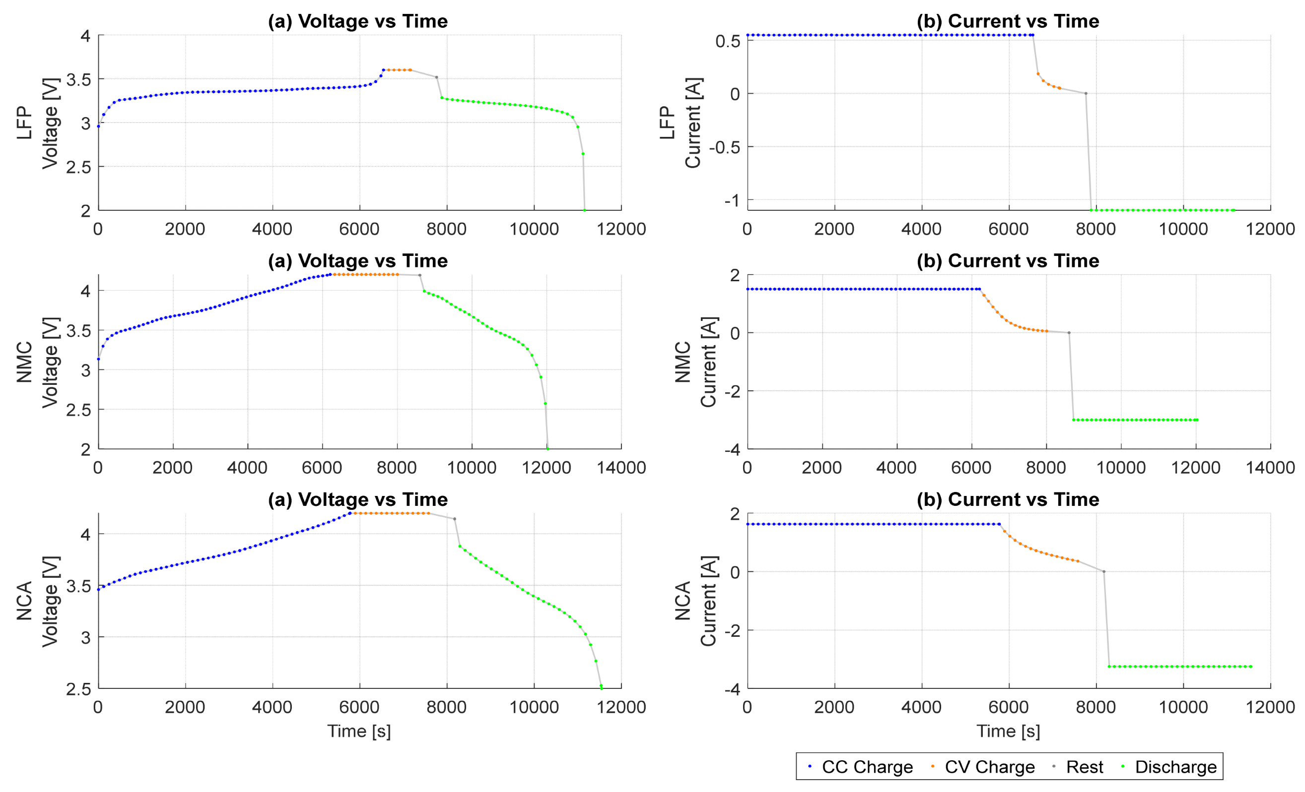
To enable phase-specific feature extraction, the cycling data were segmented into four distinct operational phases: CC charge, CV charge, rest, and CC discharge. This was achieved by identifying transitions in current and voltage using the segmentData method of the batteryTestDataParser object [18]. This section focuses on Cycle 5, selected as a representative early-life cycle due to its minimal degradation and consistent operational behaviour across chemistries, making it ideal for illustrating the segmentation process. Each data point was tagged with its corresponding cycle and step index, allowing for proper alignment with physical battery behaviour.

Figure 4 illustrates the segmented voltage and current profiles for Cycle 5 across the three chemistries: LFP (top row), NMC (middle row), and NCA (bottom row). Each subplot presents the temporal evolution of voltage (left column) and current (right column), with operational phases color-coded as follows: CC Charge (blue), CV Charge (orange), Rest (black; limited data points), and CC Discharge (green). The visual profiles in Figure 4 were generated using a custom MATLAB plotting script.

The segmented profiles shown in Figure 4 are essential for computing phase-specific features such as charge duration, energy throughput, and voltage slope. These metrics serve as critical inputs to the AutoML-based classification pipeline, enabling the model to capture nuanced differences in electrochemical behaviour. In addition to their diagnostic value, the profiles reveal distinct operational patterns across the three chemistries.

To complement the segmented profiles in Figure 4,

Table 2. Cycle-level operational behaviour from segmented profiles (Cycle 5). See Table 1 for static descriptors.

Chemistry	Voltage Evolution	Current Profile	Phase Transition Clarity	Interpretation
LFP	Rises from ~2.5 V to ~3.6 V; sharp drop during discharge	~0.5 A; zero during CV/rest; negative during discharge	Smooth and stable	Reflects low-capacity, thermally resilient behaviour
NMC	Rises from ~2.5 V to ~4.2 V; short rest plateau; sharp discharge drop	~2 A; clear CC charge → CV charge → rest → discharge transitions	Pronounced and well-defined	Indicates high energy density and complex dynamics
NCA	Similar to NMC; peaks at ~4.2 V	~2 A; well-defined transitions	Clear and consistent	Elevated thermal response due to high voltage/current

summarises the dynamic voltage and current behaviours observed during segmented charge–rest–discharge cycles. Unlike the static descriptors presented in Table 1, this table focuses on cycle-level operational patterns, such as voltage evolution, current transitions, and phase clarity. These are that are critical for downstream feature extraction and classification.

The cycle-level insights summarised in Table 2 reinforce the operational consistency across chemistries and provide a robust foundation for extracting phase-specific features, such as duration, energy, and slope. These are critical for accurate classification. These features, and the process by which they are extracted and validated, are discussed in detail in the following section.

3.4. Cycle Exclusions and Scope Considerations

To ensure the integrity of feature extraction and prevent bias in the classification model, specific charge–discharge cycles were excluded from analysis. These exclusions were guided by domain-informed heuristics, statistical checks, and manual inspection, and fall into four main categories:

• Reference Performance Tests: These cycles, previously mentioned in Section 2.2, were periodically inserted to assess baseline performance and SoH. Although useful for benchmarking, RPTs exhibit behaviour that differs from standard cycling, particularly in voltage, current, and temperature profiles. To maintain consistency in feature extraction, they were manually identified and excluded based on known test schedules.
• Irregular or Anomalous Cycles: Cycles exhibiting unusual variations in capacity, voltage, or duration (often due to sensor dropout, protocol interruptions, or data corruption) were flagged and excluded. For example, cycles missing operational segments (e.g., absent CC or CV steps) were detected using the hDetectMissingStepCycles function, a diagnostic utility within MATLAB’s PMT [19].
• Abnormally Long-Time Intervals: Time-series data are expected to progress with consistent sampling intervals. However, extended gaps (e.g., >3600 s) between consecutive data points, typically caused by system auto-restarts, can distort temporal resolution. These anomalies were identified through time-difference analysis and visual inspection. Depending on severity, either the affected data points or entire cycles were excluded [19].
• Scope Limitation for Feature Extraction: Feature engineering and diagnostic analysis in Section 4 focus primarily on the CC charge phase. This decision reflects both practical and diagnostic considerations. While CC discharge data may also be suitable for machine learning, it was not explored in this study. Although the CV phase was excluded from ICA, DVA, and DTA diagnostics due to its flat voltage profile and limited dynamic behaviour, it was still included in the feature extraction process using MATLAB’s batteryTestFeatureExtractor. When the CV flag is enabled, the extractor computes several built-in statistical and segment-specific features from CV data. Despite operating at a higher C-rate than typically recommended, the CC charge phase remains suitable for ICA-based diagnostics, which benefit from lower noise and clearer electrochemical signatures.

To operationalise these exclusions, the ExcludedCycles property of the batteryTestDataParser object, along with a custom MATLAB script, was used to ensure that only structurally complete and representative cycles contributed to downstream feature engineering.

Table 3. Summary of Excluded Cycles by Chemistry.

Chemistry	Excluded Cycles
LFP	1–4, 503–506, 508–511, 1010–1017, 1044, 1050, 1516–1523, 2022–2029, 2344–2347, 2529, 2530–2536, 2622, 2623, 2712, 3126–3134, 3633–3636
NMC	1–4, 253–256, 258–261, 386–393, 484, 518–525, 650–657, 782–785
NCA	1–4, 254–257, 259–262, 274, 314, 316, 387–394, 405, 446, 519–522

summarises the specific cycle indices excluded for each chemistry, based on the criteria outlined above. These lists were curated using a combination of automated detection methods and manual review of time-series plots and cycle-level metrics. This systematic exclusion process ensures high fidelity in feature computation and robust chemistry classification.

With segmentation and cycle exclusions complete, the next step involved feature engineering and extraction using MATLAB’s batteryTestFeatureExtractor, configured to operate on the charge phase. This process generated a comprehensive set of diagnostic metrics derived from Incremental Capacity (IC), Differential Voltage (DV), and Differential Thermal (DT) curves. The resulting feature set, comprising statistical descriptors, segment-level indicators, and differential curve metrics, forms the foundation for the diagnostic evaluations and classification tasks presented in Section 4.

4. Diagnostic Evaluation of Engineered Features

This section provides a comprehensive evaluation of the engineered feature set prior to its integration into the AutoML module (Figure 1). It begins with curve-level analysis in Section 4.1, including limitations of ICA-derived features (Section 4.1.4). Subsequent Section 4.2, Section 4.3 and Section 4.4 examine feature quality, temporal stability, inter-feature independence, and chemistry-specific separability using unsupervised methods. These steps ensure that the feature set is robust and discriminative before applying supervised selection and classification.

4.1. Diagnostic Curve Analysis

High-resolution diagnostic curves (IC, DV, and DT) are presented across selected cycles for three target chemistries: LFP, NMC, and NCA. These curves reveal degradation patterns and electrochemical and thermal signatures, which enhance model interpretability and classification accuracy.

All diagnostic curves and features discussed in this section were extracted using MATLAB’s batteryTestFeatureExtractor and batteryTestDataParser functions. The feature engineering process captures a wide range of descriptors per cycle, including statistical, segment-specific, and differential metrics, which are later evaluated for their diagnostic relevance and separability.

To consolidate insights and avoid redundancy,

Table 4. Diagnostic curve characteristics across the target chemistries, summarising key electrochemical and thermal signatures extracted from IC, DV, and DT analyses.

Chemistry	IC Curve Characteristics	DV Curve Characteristics	DT Curve Characteristics
LFP	Sharp, narrow peak near 3.4 V; stable across cycles	Single sharp peak near 3.4 V; narrow width	Flat and stable; minimal heat generation
NMC	Broad, complex peaks between 3.6–4.1 V; overlapping transitions	Multiple overlapping peaks around 3.7–4.1 V	Moderate thermal gradients; peaks near 3.8–4.1 V
NCA	Sharp transitions; prominent peak near 3.8–4.2 V	Sharper transitions than NMC; high peak slopes	Highest thermal sensitivity; sharp peaks near 4.2 V

summarises the key diagnostic characteristics observed across the target chemistries.

4.1.1. Incremental Capacity Curves Across Cycles

IC curves, derived from ICA, visualise the derivative of capacity with respect to voltage (ΔQ/ΔV). These high-resolution profiles reveal phase transitions, reaction kinetics, and ageing-related degradation mechanisms in Li-ion cells.

Figure 5 presents three-dimensional (3D) IC curves for the target chemistries across selected cycles. Each curve visualises the evolution of ΔQ/ΔV as a function of voltage over time, revealing how electrochemical processes evolve throughout the cycling lifespan.

As summarised in Table 4, the IC peak characteristics vary distinctly across chemistries. LFP shows a sharp and narrow peak near 3.4 V, NMC displays broader and overlapping transitions between 3.6–4.1 V, and NCA exhibits sharper transitions with a prominent peak near 3.8–4.2 V. These patterns evolve with ageing and reflect chemistry-specific degradation pathways.

The evolution of IC features, such as peak position, height, width, and slope, offers a rich set of descriptors for both classification and degradation assessment. These features effectively capture ageing-related shifts and are especially valuable for distinguishing chemistries with similar voltage profiles but distinct phase transition behaviours. Within the AutoML framework, IC-derived metrics significantly enhance model performance, particularly when integrated with DV and DT features to capture complementary electrochemical and thermal characteristics.

4.1.2. Differential Voltage Curves Across Cycles

DV analysis provides a high-resolution view of voltage response to incremental changes in charge (ΔV/ΔQ), offering insights into reaction kinetics, phase transitions, and internal resistance evolution. These curves are particularly useful for detecting subtle electrochemical shifts that may not be visible in raw voltage profiles.

The 3D DV curves shown in Figure 6 illustrate voltage behaviour across selected cycles for LFP, NMC, and NCA chemistries. As summarised in Table 4, LFP typically exhibits a single sharp peak near 3.4 V, NMC displays broader overlapping transitions around 3.7–4.1 V, and NCA reveals sharper transitions with steeper peak slopes. These distinctions help differentiate chemistries with overlapping voltage ranges by exposing unique electrochemical signatures.

The evolution of DV features, such as peak broadening, shifting, and flattening, serves as a proxy for degradation. Within the AutoML framework, DV-derived metrics, including peak width, slope, and prominence area, enhance model accuracy and interpretability by capturing nuanced electrochemical behaviour.

4.1.3. Differential Thermal Curves Across Cycles

DT analysis examines the rate of temperature change with respect to voltage (dT/dV), offering insights into thermal dynamics, heat generation mechanisms, and internal resistance evolution during cycling. These curves are particularly valuable for assessing safety-related behaviour and identifying chemistry-specific thermal signatures.

Figure 7, generated using MATLAB’s diagnostic pipeline, visualises temperature gradients across selected cycles for the three chemistries. As outlined in Table 4, LFP curves remain relatively flat and stable, NMC shows moderate thermal gradients with peaks near 3.8–4.1 V, and NCA demonstrates the highest thermal sensitivity, with sharp peaks near 4.2 V. These thermal descriptors help distinguish chemistries that share voltage characteristics but differ in heat generation and dissipation patterns.

The evolution of DT features, such as peak amplitude, width, and area, provides a thermal fingerprint unique to each chemistry. DT-derived metrics significantly enhance classification robustness, especially when integrated with voltage and current descriptors to capture multi-modal electrochemical behaviour. These thermal descriptors are particularly important for second-life applications where thermal stability is critical, helping identify cells with safe and predictable heat profiles under extended use.

4.1.4. Annotated IC Curve Features for Cycle 5

To illustrate the diagnostic value of IC features, Figure 8 shows annotated IC curves for Cycle 5 across the target chemistries. Each plot highlights key descriptors such as the main peak, peak width, and left/right slopes. These reflect phase transitions and reaction kinetics unique to each chemistry. LFP exhibits a sharp peak near 3.4 V, NMC shows multiple broader peaks around 3.7 V, and NCA presents a prominent peak near 3.8 V.

The most prominent peak in each curve forms the basis for computing descriptors such as position, width, slope, and prominence. This standardised approach ensures consistency and supports comparative analysis across chemistries. Validated by literature [7,14], these IC-derived features contribute significantly to the AutoML classification framework.

Although the extraction process is fully automated using MATLAB’s batteryTestFeatureExtractor and batteryTestDataParser, the computed feature values are influenced by the tuning of diagnostic parameters, such as smoothing thresholds and peak detection logic. As illustrated in Figure 8, small variations in these settings may affect feature consistency across chemistries and ageing conditions, potentially introducing variability in the PMT feature extraction process.

To address this, Section 4.2 and Section 4.3 were included to confirm the quality and reliability of the extracted features before passing them into the AutoML pipeline. Section 4.2 examines their temporal evolution across cycles and chemistries, while Section 4.3 evaluates interdependencies and separability using correlation analysis and Principal Component Analysis (PCA). Together, these steps help ensure that the feature set is both diagnostically relevant and statistically robust.

The diagnostic features extracted from IC, DV, and DT curves are grounded in well-established electrochemical principles. For example, the width and area of differential voltage peaks are indicative of voltage transition complexity and internal resistance changes, while the prominence and slope of thermal gradients reflect heat generation patterns associated with polarisation resistance. These characteristics provide interpretable insights into the underlying electrochemical and thermal behaviour of cells, enhancing the physical relevance of the classification framework.

4.2. Feature Grouping and Temporal Evolution

To improve clarity and interpretability, the extracted features are grouped into four diagnostic categories: IC and Current Metrics, DV Metrics, Temperature Metrics, and CV, DT, Segment, and Cycle-Level Metrics. This grouping supports targeted analysis of degradation trends and chemistry-specific behaviour. The following subsections illustrate the temporal evolution of selected features across cycles and chemistries, with each figure containing four labelled subplots (a)–(d). These features were chosen based on their visual separability, physical interpretability, and relevance to the AutoML classification pipeline. While only four representative features are visualised per group, the full set of 75 engineered features is listed in Appendix A and used in unsupervised analysis in Section 4.3 and Section 4.4.

4.2.1. IC and Current-Derived Features

Incremental Capacity (IC) features, derived from ICA (ΔQ/ΔV curves), capture electrochemical phase transitions and ageing-related shifts in reaction kinetics. Key descriptors, peak position, width, slope, and prominence, reflect internal mechanisms and evolve with degradation, offering chemistry-specific diagnostic value.

Complementing IC features, current-derived metrics provide insights into operational behaviour and ageing dynamics. The four subplots in Figure 9, labelled (a)–(d), presents selected features that exhibit clear, non-flat trends across cycles and enable physical interpretation relevant to chemistry classification and degradation tracking:

(a)

Charge_Step9_CC_energy: Shows a strong declining trend for NMC and NCA, indicating progressive capacity fade and reduced energy throughput during the current constant phase.

(b)

Charge_Step9_CC_duration: Exhibits a consistent downward trend for NMC and NCA, reflecting reduced charge acceptance time as cells age.

(c)

Charge_Step9_CCCV_energyRatio: Increases for LFP, suggesting a shift in energy delivery dynamics between CC and CV phases, while remaining stable for NMC and NCA.

(d)

Charge_Current_kurtosis: Captures changes in the shape of current distribution, with NMC and NCA showing evolving kurtosis values that may reflect ageing-induced variability in current profiles.

These features span both statistical and segment-specific domains, capturing instantaneous and cumulative behaviour. Their inclusion in the AutoML pipeline supports robust chemistry differentiation and enhances model interpretability. Spikes in LFP features may stem from diagnostic limitations discussed in Section 4.1.4. No smoothing was applied; however, cycles with extreme values were manually excluded (see Table 3) to ensure robust feature computation.

4.2.2. DV-Derived Voltage Features

Differential Voltage (DV) features, extracted from ΔV/ΔQ curves, offer high-resolution insights into voltage response and internal resistance evolution. These descriptors capture subtle electrochemical transitions that evolve with ageing and are particularly valuable for distinguishing chemistries with overlapping nominal voltage ranges.

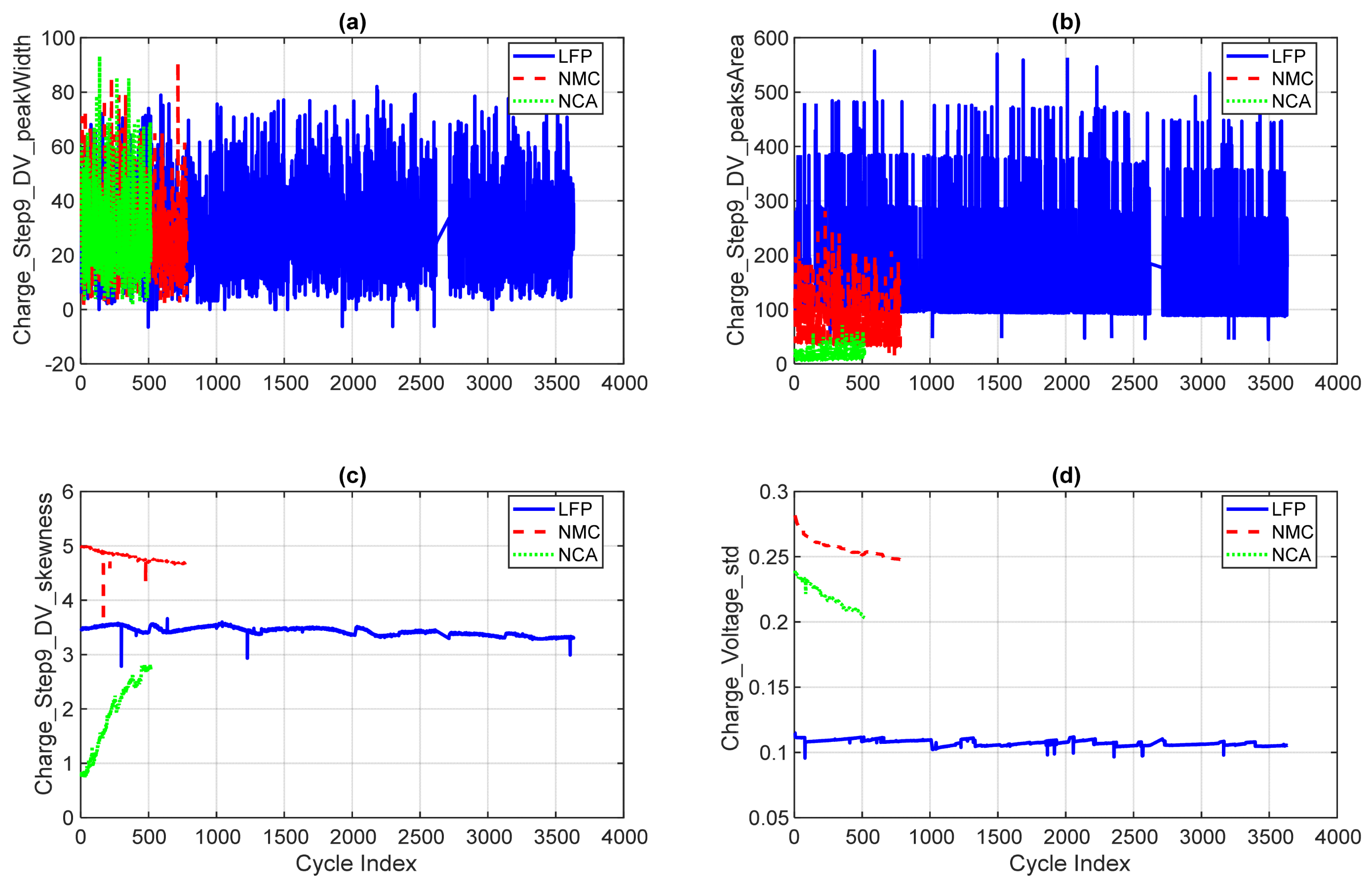
The four subplots in Figure 10, labelled (a)–(d), present DV-derived features selected based on their chemistry-specific trends, temporal consistency, and diagnostic relevance.

(a)

Charge_Step9_DV_peakWidth: Although the subplot contains dense data points leading to visual overlap, the trends remain interpretable. LFP exhibits a relatively stable DV peak width across its long cycle life, with occasional fluctuations. In contrast, NMC and NCA show higher initial peak widths that decrease and stabilise within the early cycles, reflecting ageing-related changes in voltage transition complexity.

(b)

Charge_Step9_DV_peaksArea: Captures the cumulative area under all DV peaks during charging. NMC and NCA exhibit broader transitions and increased internal resistance, while LFP remains stable and narrow across cycles.

(c)

Charge_Step9_DV_skewness: Measures the asymmetry of voltage response. NMC starts with higher skewness and gradually declines, reflecting ageing-induced shifts in reaction kinetics. LFP remains near zero, while NCA shows minimal variation.

(d)

Charge_Voltage_std: A statistical descriptor of voltage variability during charging. NMC and NCA display higher standard deviation values, while LFP maintains a low and stable profile, reinforcing its electrochemical stability.

These DV metrics, illustrated in Figure 10 subplots (a)–(d), complement the IC and current-derived features discussed in Section 4.2.1. Their inclusion enhances classification accuracy and supports robust second-life cell sorting.

4.2.3. Statistical Temperature Features

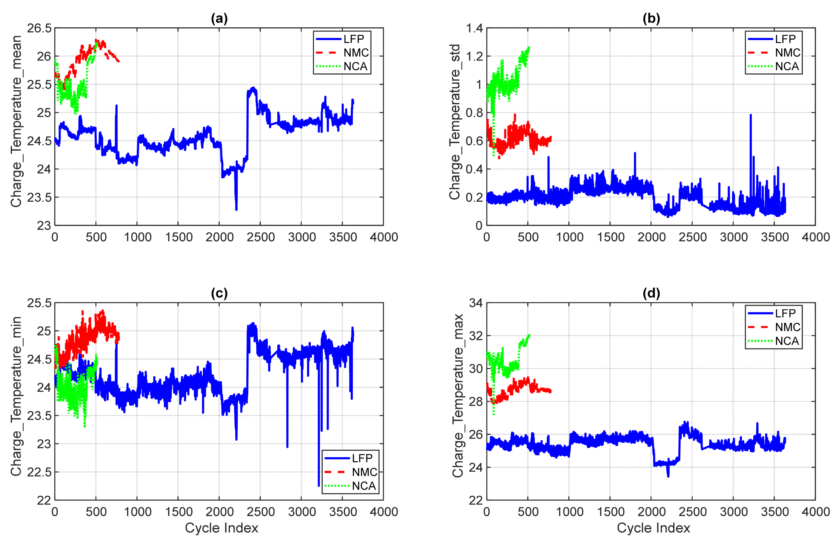
Statistical temperature descriptors provide insight into chemistry-specific thermal behaviour and ageing-related variability. The four subplots in Figure 11, labelled (a)–(d), present selected temperature features that highlight differences in thermal stability and internal resistance across LFP, NMC, and NCA chemistries:

(a)

Charge_Temperature_mean: LFP maintains a consistently low mean temperature profile, typically below 30 °C. NMC and NCA show elevated mean temperatures, with NCA reaching over 40 °C in late-life cycles, indicating higher internal resistance and thermal stress.

(b)

Charge_Temperature_std: Standard deviation values are lowest for LFP, reflecting thermal stability. NMC and NCA exhibit greater variability, with NCA showing the highest fluctuations.

(c)

Charge_Temperature_min: LFP consistently records the lowest minimum temperatures across cycles, often below 25 °C. NMC and NCA show slightly higher minimums, with occasional dips during rest phases.

(d)

Charge_Temperature_max: NCA reaches peak temperatures exceeding 45 °C in late-life cycles, while LFP remains below 35 °C.

These thermal features complement the electrochemical descriptors discussed earlier, contributing to a comprehensive diagnostic feature set used in the AutoML pipeline.

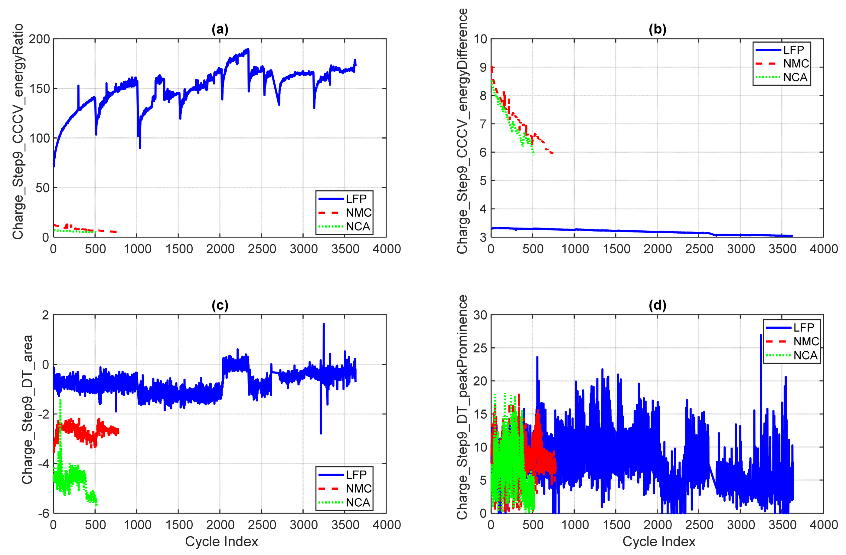
4.2.4. CV, DT, Segment, and Cycle-Level Metrics

To capture late-stage charging behaviour, thermal transitions, and electrochemical dynamics, this section focuses on four diagnostic features extracted from CV, DT, and segment-level metrics. These features were selected based on their non-linear trends, chemistry-specific separability, and physical interpretability. The corresponding subplots in Figure 12, labelled (a)–(d), illustrate their temporal evolution across cycles:

(a)

Charge_Step9_CCCV_energyRatio: Reflects the relative energy delivered during the constant current (CC) and constant voltage (CV) phases. LFP shows a rising trend, indicating a shift in energy delivery dynamics, while NMC and NCA remain relatively stable.

(b)

Charge_Step9_CCCV_energyDifference: Measures the absolute energy difference between CC and CV phases. NMC and NCA exhibit declining trends, consistent with ageing-related reductions in CV energy throughput.

(c)

Charge_Step9_DT_area: Represents the total area under the differential thermal curve, capturing cumulative heat generation. NCA shows the highest values and variability, reflecting elevated internal resistance and thermal stress.

(d)

Charge_Step9_DT_peakProminence: Quantifies the strength of the dominant thermal peak. NCA displays prominent peaks, while LFP remains flat and stable, reinforcing its thermal resilience.

While LFP cells are readily distinguishable due to their flat voltage plateau, differentiating between NMC and NCA chemistries requires more nuanced analysis. This framework leverages high-resolution differential features to capture subtle electrochemical and thermal distinctions. Specifically, NCA cells tend to exhibit narrower and more pronounced differential voltage (DV) peaks, as reflected in lower DV peak width and higher DV area values. In contrast, NMC cells display broader and more overlapping DV transitions, indicative of more complex phase behaviour. Additionally, thermal features such as DT peak prominence are typically higher in NCA cells, reflecting their elevated internal resistance and greater heat generation during cycling. These feature-level differences contribute to the model’s ability to accurately separate NMC and NCA chemistries, despite their similar nominal voltage profiles.

These features complement the IC, DV, and current-derived metrics discussed earlier, enhancing the diagnostic resolution of the AutoML pipeline and supporting robust chemistry classification, degradation tracking, and second-life suitability assessment.

4.3. Feature Correlation Analysis

To assess internal dependencies and potential redundancies within the engineered feature set, this subsection applies Pearson correlation analysis across chemistries. Identifying tightly coupled or redundant descriptors is essential for improving model interpretability, reducing dimensionality, and guiding downstream feature selection. Correlation matrices were computed separately for LFP, NCA, and NMC chemistries using a custom MATLAB workflow, which involved:

• Extracting common features from segmented charge–discharge cycles;
• Applying mean imputation to handle missing values;
• Calculating pairwise correlations using MATLAB’s corr function.

The resulting heatmaps visualise relationships among features spanning four major categories:

• Statistical descriptors (e.g., mean, standard deviation, skewness);
• Cycle-cumulative metrics (e.g., capacity, energy);
• Segment-specific indicators (e.g., CC/CV durations, slopes);
• Differential curve features (e.g., IC, DV, DT profiles).

For completeness, the full list of 75 extracted features used in the correlation analysis is provided in Appendix A (

Table A1. Diagnostic feature grouping and definitions used in unsupervised analysis.

Feature Category	Feature Names
IC and Current Metrics (20 features)	Charge_Current_max, Charge_Current_min, Charge_Current_mean, Charge_Current_std, Charge_Current_skewness, Charge_Current_kurtosis, Charge_Step9_IC_peak, Charge_Step9_IC_peakWidth, Charge_Step9_IC_peakLocation, Charge_Step9_IC_peakProminence, Charge_Step9_IC_peaksArea, Charge_Step9_IC_peakLeftSlope, Charge_Step9_IC_peakRightSlope, Charge_Step9_IC_area, Charge_Step9_IC_max, Charge_Step9_IC_min, Charge_Step9_IC_mean, Charge_Step9_IC_std, Charge_Step9_IC_skewness, Charge_Step9_IC_kurtosis
DV Metrics (20 features)	Charge_Voltage_max, Charge_Voltage_min, Charge_Voltage_mean, Charge_Voltage_std, Charge_Voltage_skewness, Charge_Voltage_kurtosis, Charge_Step9_DV_peak, Charge_Step9_DV_peakWidth, Charge_Step9_DV_peakLocation, Charge_Step9_DV_peakProminence, Charge_Step9_DV_peaksArea, Charge_Step9_DV_peakLeftSlope, Charge_Step9_DV_peakRightSlope, Charge_Step9_DV_area, Charge_Step9_DV_max, Charge_Step9_DV_min, Charge_Step9_DV_mean, Charge_Step9_DV_std, Charge_Step9_DV_skewness, Charge_Step9_DV_kurtosisCharge_Voltage_max, Charge_Voltage_min, Charge_Voltage_mean, Charge_Voltage_std, Charge_Voltage_skewness, Charge_Voltage_kurtosis
Temperature Metrics (4 features)	Charge_Temperature_max, Charge_Temperature_min, Charge_Temperature_mean, Charge_Temperature_std
CV, DT, Segment, and Cycle-Level Metrics (31 features)	Charge_Step9_CV_duration, Charge_Step9_CV_energy, Charge_Step9_CV_kurtosis, Charge_Step9_CV_skewness, Charge_Step9_CV_slope, Charge_Step9_CV_voltageMedian, Charge_Step9_DT_area, Charge_Step9_DT_kurtosis, Charge_Step9_DT_max, Charge_Step9_DT_mean, Charge_Step9_DT_min, Charge_Step9_DT_peak, Charge_Step9_DT_peakLeftSlope, Charge_Step9_DT_peakLocation, Charge_Step9_DT_peakProminence, Charge_Step9_DT_peakRightSlope, Charge_Step9_DT_peakWidth, Charge_Step9_DT_peaksArea, Charge_Step9_DT_skewness, Charge_Step9_DT_std, Charge_Step9_CC_duration, Charge_Step9_CC_currentMedian, Charge_Step9_CC_energy, Charge_Step9_CC_skewness, Charge_Step9_CC_kurtosis, Charge_Step9_CCCV_energyRatio, Charge_Step9_CCCV_energyDifference, Charge_cumulativeCapacity, Charge_cumulativeEnergy, Charge_duration, Charge_startVoltage

).

LFP Chemistry: The correlation matrix for LFP in Figure 13 reveals moderate clustering among voltage and capacity-related features, suggesting shared electrochemical dependencies. However, descriptors derived from differential curves, particularly IC and DV metrics, exhibit low or negative correlations with other feature groups. This dispersed structure reflects LFP’s stable voltage plateau and thermal resilience, resulting in flatter diagnostic profiles and greater independence among features. Such loosely coupled features are advantageous for tracking subtle degradation trends and support high interpretability in classification task.

NMC Chemistry: Figure 14 presents the NMC correlation matrix, a more balanced distribution of feature interdependencies. Moderate coupling is observed across most feature groups, with differential voltage and statistical descriptors showing consistent but not excessive correlation. Temperature and segment-specific metrics exhibit a more dispersed relationship, reflecting NMC’s intermediate electrochemical behaviour: more reactive than LFP but less volatile than NCA. This balanced feature landscape supports generalisable classification with moderate dimensionality and reduced risk of redundancy.

NCA Chemistry: As shown in Figure 15, the NCA correlation matrix shows strong clustering, especially among temperature-related and CV-phase features. This pattern aligns with NCA’s elevated energy density and thermal sensitivity, which drive tighter interdependencies among thermal and electrochemical indicators. Notably, differential voltage features are strongly correlated with cumulative energy and CV metrics, indicating that sharper phase transitions and dynamic voltage behaviour contribute to feature coupling. These correlations suggest the need for careful feature pruning to avoid overfitting and ensure model generalisability.

Comparative Insights:

• LFP: Loosely coupled features with high independence, ideal for degradation tracking and interpretability.
• NCA: Balanced interdependencies across feature groups, supporting flexible and generalisable classification.
• NMC: Strong clustering in thermal and CV-phase domains, requiring targeted feature selection to reduce complexity.

These correlation insights provide a foundation for understanding feature redundancy and chemistry-specific dependencies. The next section builds on this by evaluating the separability of chemistries in reduced feature space using PCA.

4.4. PCA-Based Feature Separability Analysis

To complement the correlation analysis in Section 4.3, this subsection applies PCA to the engineered feature set to assess chemistry-specific separability in reduced dimensional space. PCA is a widely used unsupervised technique that transforms high-dimensional data into orthogonal components, enabling intuitive visualisation of variance and clustering. This analysis provides a preliminary indication of how well the diagnostic features distinguish between LFP, NMC, and NCA chemistries prior to any supervised learning or feature selection.

Before applying PCA, linearly dependent features were removed using QR decomposition to ensure the input matrix was full rank. This step improves numerical stability and avoids redundancy in the principal component space, allowing for more accurate interpretation of variance and clustering.

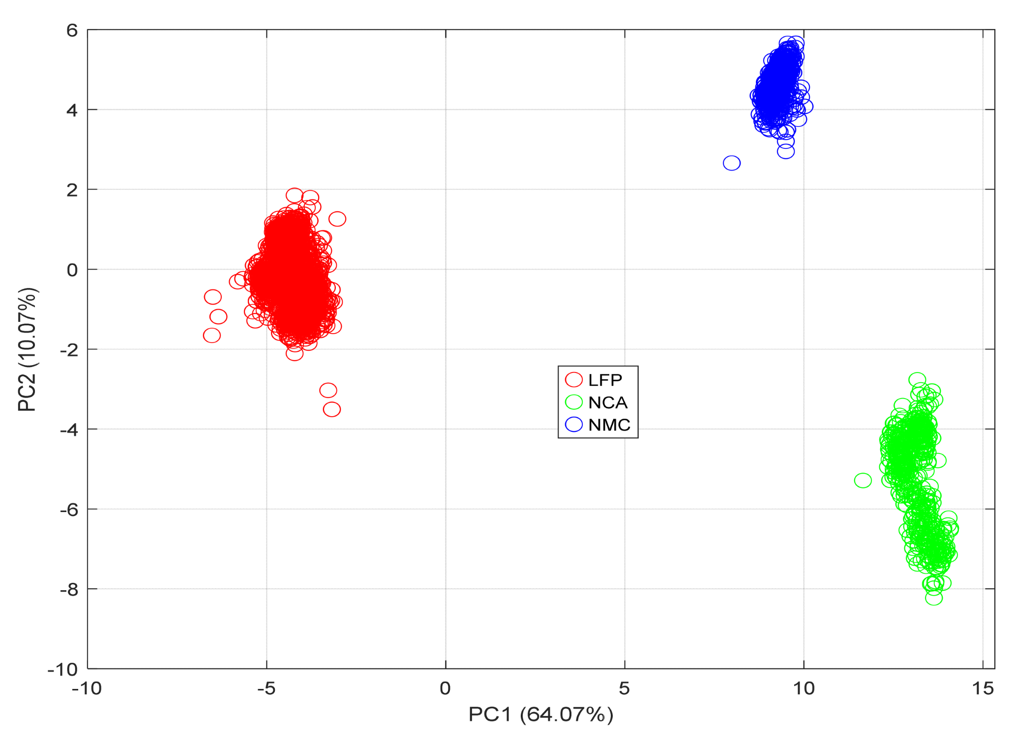
Figure 16 presents a PCA scatter plot of cycle-level feature vectors projected onto the first two principal components:

• PC1 explains 64.07% of the variance.
• PC2 explains 10.07% of the variance.

Each point represents a sample from one of the three chemistries: LFP (red), NCA (green), and NMC (blue), mapped into a two-dimensional space derived from the reduced feature set.

Observations:

The resulting clusters reveal strong chemistry-specific separability:

• LFP samples form a distinct and compact group, consistent with their stable voltage profiles, narrow IC peaks, and low thermal variability.
• NCA samples occupy an intermediate region, bridging the characteristics of LFP and NMC. Their spread reflects moderate feature coupling and a balance between electrochemical complexity and thermal behaviour.
• NMC samples form a compact cluster with slight elongation along PC1, reflecting strong internal correlations among temperature and CV-phase features.

These spatial patterns reinforce the correlation insights discussed in Section 4.3 and demonstrate the diagnostic separability of chemistries in reduced feature space.

Importantly, the PCA plot demonstrates that even without feature selection or supervised learning, the engineered descriptors, after removing linear dependencies, encode sufficient chemistry-specific variance to enable visual discrimination. This validates the effectiveness of the feature engineering pipeline and supports the feasibility of metadata-independent classification. Having confirmed the diagnostic quality and separability of the refined feature set through unsupervised analysis, the next section presents the supervised feature selection and AutoML-based classification process.

5. Automated Machine Learning

AutoML refers to a set of techniques and frameworks designed to automate the end-to-end process of applying machine learning to real-world datasets [19,20]. It eliminates the need for extensive manual intervention by automatically handling key stages such as data preprocessing, feature engineering, algorithm selection, and hyperparameter optimisation. Central to the AutoML paradigm is the resolution of the Combined Algorithm Selection and Hyperparameter optimisation (CASH) problem, which traditionally requires expert knowledge and significant trial-and-error [21,22]. Modern AutoML tools use advanced search strategies such as Bayesian optimisation, evolutionary algorithms, and meta-learning to efficiently explore large configuration spaces. This enables rapid development of high-performing models, even in complex domains such as battery chemistry classification, where the optimal pipeline is often non-trivial to identify [20,21]. An overview of the MATLAB AutoML pipeline for battery chemistry classification is shown in Figure 17 [23].

This study leveraged MATLAB’s built-in AutoML functionality, specifically the fitauto function to develop an efficient and accurate model for classifying lithium-ion battery chemistries (LFP, NCA, and NMC). The integration of AutoML into the research pipeline minimises manual bias, improves model selection transparency, and ensures the reproducibility and scalability of the results.

5.1. Data Pre-Processing

Effective data preprocessing is a crucial prerequisite for any successful machine learning pipeline, as it enhances data quality, ensures consistency, and facilitates accurate and reliable model training [20]. In this study, the preprocessing phase encompassed three key stages: data cleaning, stratified splitting, and feature normalisation. These steps were carefully selected to preserve the integrity of the original data while preparing it for subsequent stages of analysis, including feature selection and classification. To ensure full reproducibility of all results, a fixed random seed (rng(42)) was set at the beginning of the MATLAB script. This guarantees that all stochastic operations in data preparation, including stratified train/test splitting, produce identical outcomes across repeated runs.

5.2. Data Cleaning

Data cleaning refers to the process of detecting and rectifying inconsistencies or inaccuracies within a dataset, such as missing, irrelevant, or erroneous entries [20]. Prior to merging, each dataset, representing different cathode chemistries in lithium-ion batteries (specifically, LFP, NCA, and NMC was individually curated to ensure data quality.

Each dataset was assigned a numeric class label to facilitate supervised classification: LFP was labelled as 0, NCA as 1, and NMC as 2. Redundant or non-informative columns, such as Cycle_Index, were removed when present, on the basis that they did not contribute meaningful discriminatory power between classes. Additionally, columns containing exclusively missing values were discarded.

To address partially missing data, a conservative imputation strategy was employed in which missing values within numeric columns were replaced with zero. This approach was deemed appropriate given the nature of the dataset, where missing entries may correspond to negligible or non-recorded sensor outputs. This imputation ensured that no sample was excluded during training, preserving the completeness of the dataset.

5.3. Data Splitting

Following the cleaning process, each of the three class-labelled datasets was partitioned into training and testing subsets using a stratified sampling approach. Specifically, 70% of the observations within each class were randomly assigned to the training set, with the remaining 30% forming the test set. These subsets were then recombined across classes to form the final training and testing datasets.

This stratified strategy was employed to ensure that each class was proportionally represented in both the training and test sets. Such an approach mitigates the risk of model bias arising from class imbalance [13], which is a common issue in multi-class classification problems. Furthermore, by maintaining similar class distributions across splits, the performance of the classification algorithm can be more reliably evaluated on unseen data.

5.4. Data Normalisation

Normalisation is a technique used to standardise the scale of features, particularly when features exhibit differing units or magnitudes. In this study, L1 normalisation was applied to all feature vectors. Under this scheme, each feature vector (i.e., row) was scaled such that the sum of the absolute values of its components equals one [24] and can be calculated by using Equation (1).

$${\mathrm{x}}_{\mathrm{norm}}={\displaystyle \frac{\mathrm{x}}{{\sum }_i\left|{\mathrm{x}}_i\right|}}$$

(1)

This method emphasises the relative contribution of each feature within a sample, making it particularly appropriate for compositional or proportional data. Moreover, L1 normalisation is beneficial when utilising distance-based models or feature selection techniques, as it prevents features with larger scales from disproportionately influencing the model. To ensure numerical stability, special attention was given to rows where division by zero could occur (e.g., rows with all zero entries). Such cases were identified and corrected to prevent the introduction of infinite or undefined values in the processed dataset.

5.5. Feature Selection

While AutoML automates model selection and hyperparameter optimisation, feature selection in this study was performed manually using Sequential Forward Selection (SFS). This hybrid approach was chosen because, at present, MATLAB’s AutoML (fitcauto) does not natively automate feature selection. By manually applying SFS, we ensured that the most diagnostically relevant and interpretable features were selected, aligning the feature set with domain-specific knowledge and enhancing model transparency. This combination leverages the strengths of AutoML for unbiased model optimisation while retaining expert oversight in feature selection.

Feature selection is a fundamental component of any machine learning pipeline, particularly in high-dimensional datasets where redundant or irrelevant features can obscure informative patterns. In this study, the objective of feature selection was twofold: to enhance classification performance and to improve interpretability by identifying the features most relevant for distinguishing between lithium-ion battery chemistries LFP, NCA, and NMC. Reducing the feature space also serves to lower computational complexity and mitigate the risk of overfitting.

In this study, SFS was employed. It is a wrapper-based approach that evaluates subsets of features in conjunction with a predictive model. SFS adopts a greedy strategy [25,26]: it begins with an empty set and iteratively adds one feature at a time, the feature that, when added, yields the greatest reduction in classification error. Formally, at each step $k$, SFS selects the feature $f_k$ as shown in Equation (2):

$$f_k=\mathrm{a}\mathrm{r}\mathrm{g}\underset{j\notin {\mathcal{S}}_{k-1}}{\mathrm{m}\mathrm{i}\mathrm{n}} \mathcal{L}\left({\mathcal{S}}_{k-1}\cup \left\{j\right\}\right)$$

(2)

where ${\mathcal{S}}_{k-1}$ is the current set of selected features and $\mathcal{L}$ denotes the classification loss. In this study, the loss function was the cross-validated misclassification rate, providing a robust estimate of generalisation performance.

The selection process was implemented in MATLAB using the sequentialfs() function. A custom evaluation function was defined based on a multiclass Error-Correcting Output Codes (ECOC) framework, with a Support Vector Machine (SVM) as the base learner. Performance was assessed using 5-fold cross-validation, in which the training data was partitioned into five subsets, with iterative training and validation to ensure unbiased performance estimation.

To balance model simplicity and discriminative power, the number of features to be selected was capped at five. This decision was based on an empirical trade-off: selecting enough features to preserve classification accuracy, while avoiding unnecessary model complexity.

Figure 18 illustrates the reduction in cross-validation error as additional features were incorporated. The loss at each iteration k was computed as shown in Equation (3):

$$\mathrm{Loss\; at\; step} k={\displaystyle \frac{1}{n_{\mathrm{val}}}}\sum _{i=1}^{n_{\mathrm{val}}} \mathbb{I}\left({\widehat{y}}^{\left(i\right)}\ne y^{\left(i\right)}\right)$$

(3)

where ${\widehat{y}}^{\left(i\right)}$ and $y^{\left(i\right)}$ represent predicted and true class labels for sample $i$, and $\mathbb{I}(\cdot )$ is the indicator function.

As depicted in Figure 18, the error decreased steadily from 1.89 × 10⁻⁴ with the first feature to 6.08 × 10⁻⁵ after the 5th, confirming the cumulative relevance of the selected features and indicating diminishing marginal returns beyond this point.

The final feature subset comprised the following variables:

• Charge_Step9_CV_duration
• Charge_Step9_DT_peakLeftSlope
• Charge_Step9_DT_peakRightSlope
• Charge_Step9_DV_area
• Charge_duration

As shown in Figure 19, the five selected features exhibit distinct and consistent trends across LFP, NMC, and NCA chemistries. These trends reflect underlying electrochemical and thermal behaviours that are critical for classification:

• The CV duration and overall charge duration capture differences in voltage plateau behaviour and charge acceptance, with LFP showing shorter, more stable durations and NMC/NCA exhibiting longer, more variable profiles.
• The thermal slope features (left and right of the DT peak) highlight chemistry-specific heat generation patterns, with NCA showing steep gradients due to elevated internal resistance, while LFP remains thermally stable.
• The DV area reflects the complexity of voltage transitions, distinguishing LFP’s narrow, stable response from the broader, evolving profiles of NMC and NCA.

These features were selected not only for their statistical separability but also for their physical interpretability. Their consistent evolution across cycles reinforces their diagnostic value and supports their use in scalable, metadata-independent chemistry classification.

By adopting SFS, a method that directly integrates model performance into the feature selection process, this study avoids the limitations of filter-based approaches such as Laplacian Score or ReliefF, which evaluate features independently of the learning algorithm. Consequently, the selected subset is inherently aligned with the classifier’s decision boundaries, leading to more robust and tailored classification outcomes.

The selected features, such as CV duration, DV area, and DT peak slopes, are not only statistically discriminative but also physically interpretable. They correspond to electrochemical and thermal behaviours that are well-documented in literature, including voltage plateau dynamics, phase transitions, and heat dissipation characteristics. This alignment supports the model’s transparency and diagnostic value.

5.6. PCA-Based Assessment of SFS-Optimised Features

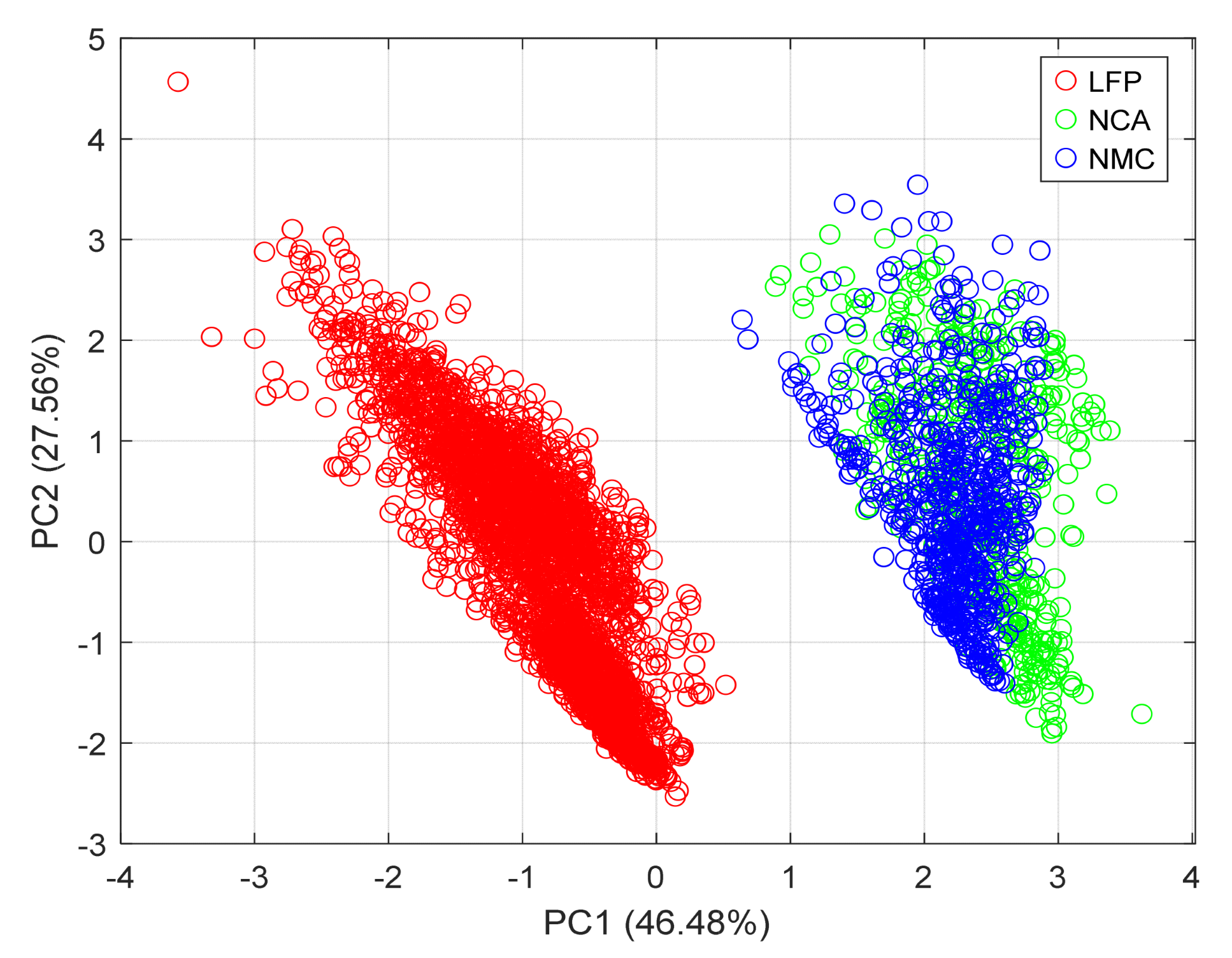
As shown in Figure 19, the selected features display clear chemistry-specific trends. To further assess their combined discriminative power, a PCA was performed using these five features. Figure 20 presents a PCA scatter plot of Li-ion battery cycling data using the five most discriminative features selected via MATLAB’s sequentialfs function. These features, comprising time-domain and derivative metrics, were chosen to minimise cross-validated misclassification loss, as detailed in Section 5.5. This dimensionality reduction was performed on a compact feature subset identified through SFS, which optimises classification performance by iteratively selecting features that improve generalisation.

The PCA projection onto the first two principal components, PC1 (46.48% variance explained) and PC2 (27.56%), reveals clear clustering of LFP, NCA, and NMC samples. Compared to the broader PCA analysis in Section 4.4, which used the full feature set, this reduced representation offers improved interpretability and computational efficiency while preserving classification robustness.

Importantly, the current analysis confirms that even a minimal, well-chosen subset retains strong chemistry-specific separability. This reinforces the diagnostic value of the selected features and supports their suitability for scalable classification workflows.

6. Results and Discussion

This section presents the outcomes of the machine learning pipeline, focusing on the impact of data preprocessing, feature selection, and AutoML optimisation on classification performance. The results are interpreted both statistically and in relation to battery chemistry, highlighting the effectiveness and relevance of the proposed approach.

6.1. AutoML Model Optimisation

Following feature selection, MATLAB’s fitcauto function was employed to automate the model selection and hyperparameter tuning process. The optimiser was configured with a maximum objective evaluation budget of 100 iterations, using Bayesian optimisation to balance exploration and exploitation in the model search space. A wide variety of learners including KNN, decision trees, ensemble methods, support vector machines, neural networks, and naïve Bayes classifiers were considered.

To ensure full reproducibility of the AutoML training and model selection process, a fixed random seed (rng(42)) was maintained for all stochastic operations, including Bayesian hyperparameter optimisation within the fitcauto function. Additionally, the AutoML evaluation budget was dynamically set using evalBudget = min(100, round(size(train_selected_x,1)/2)) to balance computational efficiency with model robustness. This approach guarantees that the AutoML search and final model selection are fully reproducible across repeated runs and computing environments.

Figure 21 illustrates the optimisation trajectory of the AutoML process, tracking both the observed and estimated validation losses across 100 iterations. The observed minimum validation loss eventually stabilised at L_min = 2.9472 × 10⁻⁴, indicating that the optimiser successfully identified a high-performing model configuration. Despite some fluctuations in the estimated loss during the middle stages of the search, the observed loss remained consistently low, suggesting that the final model generalised well. The integration of cross-validation in the evaluation strategy further ensured robustness and mitigated the risk of overfitting.

Despite several models achieving comparable loss values, the optimiser selected a K-Nearest Neighbours (KNN) model with a single neighbour and inverse distance weighting as the final best performer; the KNN model was favoured for its lower estimated generalisation error and reduced computational complexity, as reflected in the estimated loss L = 4.3482 × 10⁻⁴. This outcome underscores the strength of AutoML in identifying not just the best-performing model during training, but one that balances performance, stability, and efficiency.

6.2. Classification Performance: Confusion Matrix Analysis

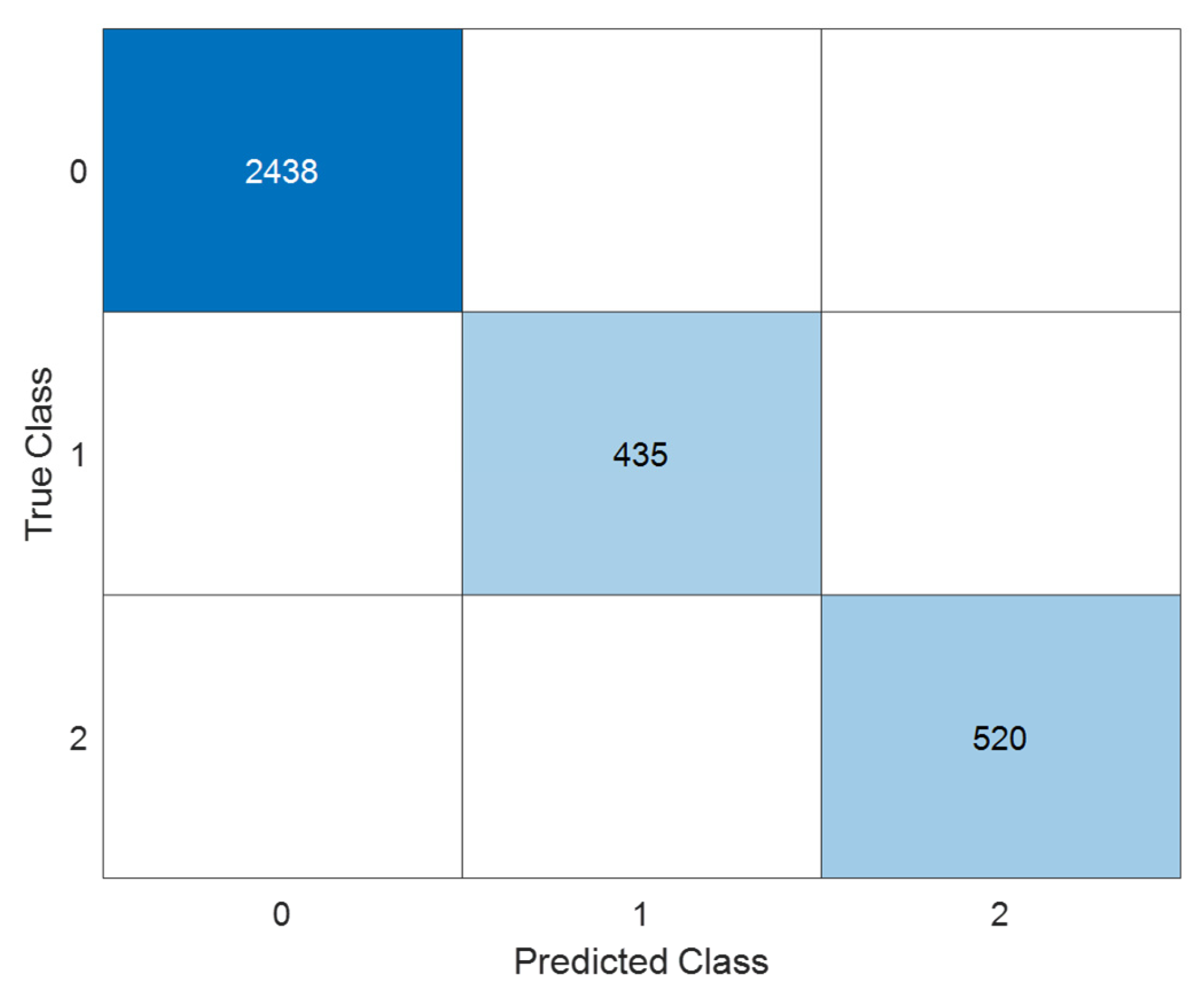
The classification performance of the trained KNN model was evaluated on both the training and test datasets using confusion matrices, providing insight into class-wise prediction accuracy and potential misclassification patterns across the three battery chemistries: LFP (class 0), NCA (class 1), and NMC (class 2).

6.2.1. Training Set

The confusion matrix for the training data shown in Figure 22 demonstrates perfect classification performance, with the model correctly identifying all 2438 LFP instances, 435 NCA instances, and 520 NMC instances. No misclassifications are observed, yielding an overall training accuracy of 100%. This level of precision suggests that the model has successfully learned the distinguishing patterns in the training data, aided by effective feature selection and optimised hyperparameters. However, such high accuracy on the training set also warrants careful validation against the test set to assess generalisability and avoid overfitting.

6.2.2. Test Set

Evaluation on the test data shown in Figure 23, comprising previously unseen instances, yielded a test accuracy of 99.93%, confirming the model’s strong generalisation capability. The test confusion matrix reveals the following insights:

• LFP (class 0): Out of 1045 samples, all were correctly classified (100% recall and precision), indicating excellent robustness in identifying this chemistry type.
• NCA (class 1): All 186 instances were accurately predicted, again yielding perfect recall and precision for this class. This is particularly notable given that NCA can sometimes exhibit overlapping electrochemical features with NMC in raw data.
• NMC (class 2): Of the 223 NMC samples, 222 were correctly classified, with only one instance misclassified as NCA. This represents a misclassification rate of less than 0.45%, which is negligible but could suggest minor feature overlap or class imbalance in edge cases.

Using only the five most discriminative features selected via SFS, namely CV duration, DV area, DT peak left slope, DT peak right slope, and overall charge duration, the model maintained near-perfect classification performance, achieving a test accuracy of 99.93%. This demonstrates that a compact and interpretable feature subset can deliver high classification accuracy while reducing model complexity and improving transparency. These results confirm that the selected features capture chemistry-specific electrochemical and thermal behaviours critical for robust classification.

The results across both sets suggest a highly discriminative model, with no significant signs of underfitting or overfitting. The successful prediction of all three classes with near-perfect accuracy underlines the suitability of the selected features identified via SFS and the effectiveness of the AutoML optimisation in configuring the most appropriate classification algorithm.

In practical terms, the model demonstrates high reliability for automated battery chemistry classification, offering substantial promise for integration into quality assurance or diagnostic systems within battery manufacturing pipelines. The consistency across class boundaries also indicates that the features selected capture chemically meaningful variations relevant to battery behaviour.

6.3. Limitations and Future Work

While the proposed AutoML framework demonstrates high accuracy and robustness for chemistry classification using long-term cycling data, several limitations and opportunities for improvement remain:

• Feature Engineering and Validation: The current feature set, although comprehensive, could be further improved by applying more constrained feature engineering and rigorous validation to ensure that only the most physically meaningful and robust features are used for classification.
• Short-Duration Measurement Data: The present study focuses on long-term cycling data. Adapting the framework to enable accurate classification using short-duration or partial cycling measurements would greatly enhance its applicability for rapid diagnostics and industrial workflows.
• Cyclability Assumption and Non-Cycling Diagnostics: The current framework assumes that cells are cyclable to some extent, enabling feature extraction from charge–discharge data. In practical second-life workflows, most candidate cells undergo pre-screening to exclude non-functional or severely degraded units before diagnostic testing. However, this assumption limits applicability to only partially functional cells. Future work could extend the framework to incorporate non-cycling diagnostic methods, such as impedance spectroscopy or rest-phase voltage analysis, to enable classification of cells that cannot be cycled.
• Diverse Operating Conditions: The model was trained and validated on research-grade datasets under controlled conditions. Future work should focus on improving model classification accuracy under a wider range of operating conditions, including varying temperatures, cycling rates, and real-world industrial datasets.
• Degradation Mode Classification: While this work addresses chemistry classification, extending the approach to also classify cell degradation modes would provide valuable insights for second-life assessment and predictive maintenance.
• Generalisation to Out-of-Distribution Scenarios: Although the proposed framework demonstrates high classification accuracy across three chemistries under standardised cycling conditions, its performance under out-of-distribution (OOD) scenarios, such as different form factors, manufacturers, or degradation trajectories, remains to be evaluated. Future work will focus on validating the model using diverse datasets that reflect real-world variability in second-life and recycling contexts. This will help assess the robustness and generalisation capability of the framework beyond the current scope.
• Beyond technical performance: The proposed framework contributes to sustainable battery lifecycle management. By enabling accurate chemistry classification without reliance on manufacturer metadata, it supports rapid second-life qualification, safe module matching, and efficient recycling pretreatment. These capabilities align with circular economy principles and help reduce electrochemical waste in large-scale battery deployment.

7. Conclusions

This article demonstrates the efficacy of automated machine learning (AutoML) in accurately classifying lithium-ion battery chemistries: specifically, LFP, NCA, and NMC, based on electrochemical features. The integration of a fully automated pipeline, comprising rigorous data preprocessing, sequential forward feature selection, and Bayesian hyperparameter optimisation within AutoML, resulted in a test classification accuracy of 99.93%. This approach reduces dependence on expert-driven parameter tuning and model selection, thereby minimising human bias and enabling a data-centric modelling paradigm.

Beyond achieving high classification accuracy, the AutoML framework facilitated the identification of influential features within the dataset. The selected attributes included time-based and derivative metrics derived from charge steps, which were consistently prioritised across multiple modelling iterations. Although the precise physical interpretation of these features may require further electrochemical analysis, their consistent selection suggests underlying patterns that are potentially meaningful and reproducible. This outcome enhances model interpretability and provides a valuable starting point for further investigation by domain experts.

From a practical perspective, this automated and reproducible methodology has strong implications for industry. It can be deployed in battery manufacturing lines for real-time cell classification, integrated into second-life battery management systems for effective module matching, and utilised in recycling facilities for accurate chemistry sorting. Ultimately, this contributes to improved safety, efficiency, and sustainability in the battery lifecycle.

Looking ahead, future work will focus on (a) improving feature quality through constrained feature engineering and validation, (b) enabling classification using short-duration measurement data, (c) enhancing model accuracy under diverse operating conditions and with industrial datasets, and (d) extending the framework to address cell degradation mode classification. These directions will further strengthen the generalisability and industrial relevance of the proposed AutoML-based battery classification pipeline. The framework’s scalability, interpretability, and metadata independence make it well-suited for integration into industrial workflows. It can support sustainable second-life battery deployment, enhance recycling efficiency, and facilitate materials discovery under limited data conditions. These broader applications underscore the societal and environmental relevance of the proposed AutoML-based classification pipeline.

References

1. IEA. Global EV Outlook; IEA: Paris, France, 2024; Available online: https://www.iea.org/reports/global-ev-outlook-2024 (accessed on 23 October 2025).
2. Harper, G.; Sommerville, R.; Kendrick, E.; Driscoll, L.; Slater, P.; Stolkin, R.; Walton, A.; Christensen, P.; Heidrich, O.; Lambert, S.; et al. Recycling Lithium-Ion Batteries from Electric Vehicles. Nature 2019, 575, 75–86. [Google Scholar] [CrossRef]
3. Martinez-Laserna, E.; Sarasketa-Zabala, E.; Villarreal Sarria, I.; Stroe, D.I.; Swierczynski, M.; Warnecke, A.; Timmermans, J.M.; Goutam, S.; Omar, N.; Rodriguez, P. Technical Viability of Battery Second Life: A Study from the Ageing Perspective. IEEE Trans. Ind. Appl. 2018, 54, 2703–2713. [Google Scholar] [CrossRef]
4. Berecibar, M.; Gandiaga, I.; Villarreal, I.; Omar, N.; Van Mierlo, J.; Van Den Bossche, P. Critical Review of State of Health Estimation Methods of Li-Ion Batteries for Real Applications. Renew. Sustain. Energy Rev. 2016, 56, 572–587. [Google Scholar] [CrossRef]
5. Meddings, N.; Heinrich, M.; Overney, F.; Lee, J.S.; Ruiz, V.; Napolitano, E.; Seitz, S.; Hinds, G.; Raccichini, R.; Gaberšček, M.; et al. Application of Electrochemical Impedance Spectroscopy to Commercial Li-Ion Cells: A Review. J. Power Sources 2020, 480, 228742. [Google Scholar] [CrossRef]
6. Zhao, Y.; Zhang, W.; Hu, E.; Yan, Q.; Xiang, C.; Tseng, K.J.; Niyato, D. BatSort: Enhanced Battery Classification with Transfer Learning for Battery Sorting and Recycling. In Proceedings of the 2024 IEEE Annual Congress on Artificial Intelligence of Things (AIoT), Melbourne, Australia, 24–26 July 2024. [Google Scholar]
7. Thompson, N.; Cohen, T.; Alamdari, S.; Hsu, C.-W.; Williamson, G.; Beck, D.; Holmberg, V. DiffCapAnalyzer: A Python Package for Quantitative Analysis of Total Differential Capacity Data. J. Open Source Softw. 2020, 5, 2624. [Google Scholar] [CrossRef]
8. Neubauer, J.; Smith, K.; Wood, E.; Pesaran, A. Identifying and Overcoming Critical Barriers to Widespread Second Use of PEV Batteries; National Renewable Energy Lab (NREL): Golden, CO, USA, 2015. [Google Scholar]
9. Lucaferri, V.; Quercio, M.; Laudani, A.; Riganti Fulginei, F. A Review on Battery Model-Based and Data-Driven Methods for Battery Management Systems. Energies 2023, 16, 7807. [Google Scholar] [CrossRef]
10. Odinsen, E.; Amiri, M.N.; Burheim, O.S.; Lamb, J.J. Estimation of Differential Capacity in Lithium-Ion Batteries Using Machine Learning Approaches. Energies 2024, 17, 4954. [Google Scholar] [CrossRef]
11. Amuta, O.; Yao, J.; Droese, D.; Kowal, J. Accurate Chemistry Identification of Lithium-Ion Batteries Based on Temperature Dynamics with Machine Learning. Batteries 2025, 11, 208. [Google Scholar] [CrossRef]
12. Karaoğlu, G.; Ulgut, B. Battery Chemistry Prediction with Short Measurements and a Decision Tree Algorithm: Sorting for a Proper Recycling Process. J. Energy Storage 2023, 72, 108232. [Google Scholar] [CrossRef]
13. Wett, C.; Lampe, J.; Görick, D.; Seeger, T.; Turan, B. Identification of Cell Chemistries in Lithium-Ion Batteries: Improving the Assessment for Recycling and Second-Life. Energy AI 2025, 19, 100468. [Google Scholar] [CrossRef]
14. Preger, Y.; Barkholtz, H.M.; Fresquez, A.; Campbell, D.L.; Juba, B.W.; Romàn-Kustas, J.; Ferreira, S.R.; Chalamala, B. Degradation of Commercial Lithium-Ion Cells as a Function of Chemistry and Cycling Conditions. J. Electrochem. Soc. 2020, 167, 120532. [Google Scholar] [CrossRef]
15. Barkholtz, H.M.; Fresquez, A.; Chalamala, B.R.; Ferreira, S.R. A Database for Comparative Electrochemical Performance of Commercial 18650-Format Lithium-Ion Cells. J. Electrochem. Soc. 2017, 164, A2697–A2706. [Google Scholar] [CrossRef]
16. Liu, K.; Peng, Q.; Che, Y.; Zheng, Y.; Li, K.; Teodorescu, R.; Widanage, D.; Barai, A. Transfer Learning for Battery Smarter State Estimation and Ageing Prognostics: Recent Progress, Challenges, and Prospects. Adv. Appl. Energy 2023, 9, 100117. [Google Scholar] [CrossRef]
17. BatteryArchive.Org. Available online: https://www.batteryarchive.org/study_summaries.html (accessed on 6 September 2025).
18. Data Analysis and Feature Extraction for Battery Raw Cycling Data—MATLAB & Simulink. Available online: https://uk.mathworks.com/help/predmaint/ug/data-analysis-and-feature-extraction-for-battery-raw-cycling-data.html (accessed on 6 September 2025).
19. Luo, C.; Zhang, Z.; Qiao, D.; Lai, X.; Li, Y.; Wang, S. Life Prediction under Charging Process of Lithium-Ion Batteries Based on AutoML. Energies 2022, 15, 4594. [Google Scholar] [CrossRef]
20. Barbudo, R.; Ventura, S.; Romero, J.R. Eight Years of AutoML: Categorisation, Review and Trends. Knowl. Inf. Syst. 2023, 65, 5097–5149. [Google Scholar] [CrossRef]
21. He, X.; Zhao, K.; Chu, X. AutoML: A Survey of the State-of-the-Art. Knowl. Based Syst. 2021, 212, 106622. [Google Scholar] [CrossRef]
22. Santu, S.K.K.; Hassan, M.M.; Smith, M.J.; Xu, L.; Zhai, C.; Veeramachaneni, K. AutoML to Date and Beyond: Challenges and Opportunities. ACM Comput. Surv. 2022, 54, 1–36. [Google Scholar]
23. AutoML Explained. Automated Machine Learning—MATLAB & Simulink. Available online: https://uk.mathworks.com/discovery/automl.html (accessed on 22 September 2025).
24. Friedman, L.; Komogortsev, O.V. Assessment of the Effectiveness of Seven Biometric Feature Normalization Techniques. IEEE Trans. Inf. Forensics Secur. 2019, 14, 2528–2536. [Google Scholar] [CrossRef]
25. Kumar, A.; Kaur, A.; Singh, P.; Driss, M.; Boulila, W. Efficient Multiclass Classification Using Feature Selection in High-Dimensional Datasets. Electronics 2023, 12, 2290. [Google Scholar] [CrossRef]
26. Chotchantarakun, K. Optimizing Sequential Forward Selection on Classification Using Genetic Algorithm. Informatica 2023, 47, 81–90. [Google Scholar] [CrossRef]
Figure 1. Workflow of the AutoML-based pipeline for classifying Li-ion battery cell chemistries.
Energies 18 05738 g001
Figure 2. Time-series profiles of current, voltage, and temperature for LFP, NMC, and NCA chemistries under identical cycling conditions (25 °C, 0–100% DoD, 0.5 C–1 C charge/discharge rates).
Energies 18 05738 g002
Figure 3. Current, voltage, and temperature profiles for early- and late-life cycles of LFP, NMC, and NCA cells.
Energies 18 05738 g003
Figure 4. Segmented voltage and current profiles for Cycle 5 across LFP, NMC, and NCA chemistries.
Energies 18 05738 g004
Figure 5. IC curves for cells from the target chemistries across selected cycles, illustrating phase transitions and degradation patterns relevant to chemistry classification.
Energies 18 05738 g005
Figure 6. DV curves for cells from the target chemistries across selected cycles, visualising voltage response to incremental charge and highlighting phase transition behaviour and electrochemical differences.
Energies 18 05738 g006
Figure 7. DT curves for cells from the target chemistries across selected cycles, visualising temperature gradients and chemistry-specific thermal behaviour during cycling.
Energies 18 05738 g007
Figure 8. Annotated IC curves for Cycle 5 across targeted chemistries, highlighting diagnostic features including peak positions, widths, and slopes used for feature extraction and classification.
Energies 18 05738 g008
Figure 9. Cycle-wise evolution of current-derived features for LFP, NMC, and NCA chemistries. Subplots (ad) show: (a) Charge_Step9_CC_energy, (b) Charge_Step9_CC_duration, (c) Charge_Step9_CCCV_energyRatio, and (d) Charge_Current_kurtosis. These features reflect ageing-related changes in energy throughput, charge duration, phase energy balance, and current distribution, supporting chemistry classification and degradation tracking.
Energies 18 05738 g009
Figure 10. Cycle-wise trends of selected DV-derived voltage features for LFP, NMC, and NCA chemistries. Subplots (ad) show: (a) Charge_Step9_DV_peakWidth, (b) Charge_Step9_DV_peaksArea, (c) Charge_Step9_DV_skewness, and (d) Charge_Voltage_std. These features capture voltage transition complexity, cumulative electrochemical activity, asymmetry in voltage response, and variability in charge voltage, supporting chemistry-specific classification and ageing analysis.
Energies 18 05738 g010
Figure 11. Cycle-wise evolution of statistical temperature features for LFP, NMC, and NCA chemistries. Subplots (ad) show: (a) Charge_Temperature_mean, (b) Charge_Temperature_std, (c) Charge_Temperature_min, and (d) Charge_Temperature_max. These features reflect chemistry-specific thermal behaviour and ageing-related variability, supporting classification and second-life suitability assessment.
Energies 18 05738 g011
Figure 12. Cycle-wise evolution of selected diagnostic features for LFP, NMC, and NCA chemistries. Subplots (ad) illustrate: (a) Charge_Step9_CCCV_energyRatio, (b) Charge_Step9_CCCV_energyDifference, (c) Charge_Step9_DT_area, and (d) Charge_Step9_DT_peakProminence. These metrics capture energy delivery dynamics, cumulative heat generation, and thermal peak strength, supporting chemistry-specific classification.
Energies 18 05738 g012
Figure 13. Pearson correlation matrix for LFP features. Voltage and capacity metrics show moderate clustering, while IC, DV, and DT descriptors exhibit low correlation, indicating high diagnostic diversity.
Energies 18 05738 g013
Figure 14. Pearson correlation matrix for NMC chemistry. Feature interdependencies are balanced across statistical, segment-specific, and differential metrics, supporting generalisable classification with moderate dimensionality.
Energies 18 05738 g014
Figure 15. Pearson correlation matrix for NCA chemistry. Strong clustering is evident among temperature-related and CV-phase features, reflecting high thermal sensitivity and tighter coupling of electrochemical indicators.
Energies 18 05738 g015
Figure 16. PCA scatter plot of cycle-level features for LFP, NMC, and NCA chemistries. Samples are projected onto PC1 and PC2, showing distinct clustering and chemistry-specific separability.
Energies 18 05738 g016
Figure 17. Overview of the MATLAB AutoML pipeline for battery chemistry classification [23].
Energies 18 05738 g017
Figure 18. Reduction in cross-validation error during SFS, showing diminishing returns after five features.
Energies 18 05738 g018
Figure 19. Cycle-wise evolution of the five SFS-selected features for LFP, NMC, and NCA. Each feature exhibits distinct chemistry-specific trends, supporting their selection for classification.
Energies 18 05738 g019
Figure 20. PCA scatter plot using five most discriminative features selected via SFS. Shows effective classification potential.
Energies 18 05738 g020
Figure 21. AutoML optimisation trajectory showing observed and estimated validation losses across 100 iterations.
Energies 18 05738 g021
Figure 22. Confusion matrix for training set.
Energies 18 05738 g022
Figure 23. Confusion matrix for test set.
Energies 18 05738 g023