Abstract
Conventional power load forecasting frameworks face limitations in dynamic spatial topology capture and long-term dependency modeling. To address these issues, this study proposes a hybrid GAT-CNN-LSTM architecture for enhanced short-term power load forecasting. The model integrates three core components synergistically: Graph Attention Network (GAT) dynamically captures spatial correlations via adaptive node weighting, resolving static topology constraints; a CNN-LSTM module extracts multi-scale temporal features—convolutional kernels decompose load fluctuations, while bidirectional LSTM layers model long-term trends; and a gated fusion mechanism adaptively weights and fuses spatio-temporal features, suppressing noise and enhancing sensitivity to critical load periods. Experimental validations on multi-city datasets show significant improvements: the model outperforms baseline models by a notable margin in error reduction, exhibits stronger robustness under extreme weather, and maintains superior stability in multi-step forecasting. This study concludes that the hybrid model balances spatial topological analysis and temporal trend modeling, providing higher accuracy and adaptability for STLF in complex power grid environments.
1. Introduction
1.1. General Introduction
With the evolution of new power systems, the integration of diversified loads, high-penetration renewable energy, and the inherent stochasticity and volatility of renewables have significantly increased the complexity of load patterns. Power load forecasting is a technical framework that scientifically estimates future electricity demand (including power and energy consumption) for specific timepoints or periods within a power system. It leverages multi-source information such as historical consumption data, meteorological conditions, and socio-economic activities, employing mathematical models and intelligent algorithms [1]. The core objectives are to optimize resource allocation, ensure grid security, and enhance energy efficiency by analyzing load variation patterns. Based on temporal scales, power load forecasting is categorized into long-term, medium-term, and short-term forecasting. Effective short-term power load forecasting (STLF) enables grid operators to proactively plan generation scheduling, rationally arrange reserve capacity, minimize economic losses caused by prediction deviations, and maximize the utilization of clean energy [2].
In recent years, significant progress has been made in system-level and regional-level power load forecasting research. Artificial intelligence methodologies, particularly machine learning (ML) and deep learning (DL), have facilitated the development of predictive models such as Support Vector Machines (SVM) [3], Random Forests (RF) [4], and Artificial Neural Networks (ANN) [5]. Nevertheless, ANN models exhibits inherent limitations: they struggle to capture intrinsic correlations within sequential data, often requiring manual extraction of temporal features from historical load data to establish input-output mappings.
Power load sequences are characterized by nonlinearity, non-stationarity, and dynamic evolution, meaning current outputs depend not only on immediate inputs but also on historical states. Manual feature engineering disrupts the temporal continuity of load data, while simplistic input-output mappings further compromise prediction accuracy.
1.2. Motivation and Gap
To address these challenges, DL algorithms have gained prominence in load forecasting. Sequential modeling techniques—including Recurrent Neural Networks (RNN) [6], Convolutional Neural Networks (CNN) [7], Long Short-Term Memory networks (LSTM) [8], alongside emerging architectures like Transformers and Graph Neural Networks (GNN) [9] have been progressively integrated into this domain. RNNs, with their cyclic structure enabling implicit state transmission across time steps, significantly enhance the modeling of temporal dependencies, making them particularly effective for processing dynamic power load sequences.
Reference [10] explores machine learning applications in short-term load forecasting, emphasizing their superiority over traditional methods in handling nonlinear load patterns and complex factors like weather and socioeconomic conditions. The article highlights deep learning models, particularly LSTM networks, for capturing temporal dependencies, and discusses hybrid approaches combining ML with statistical techniques to enhance accuracy. Key challenges include data quality, model interpretability, and computational efficiency. Practical implementation insights focus on feature selection, hyperparameter tuning, and ensemble methods. The study underscores ML’s potential to achieve high forecasting precision while addressing real-world constraints like outlier sensitivity and non-stationary data. Emerging trends like attention mechanisms and optimization algorithms are noted for future research directions. Reference [11] propose a short-term load forecasting model combining Temporal Convolutional Network with channel and temporal attention mechanisms to capture nonlinear relationships between meteorological factors and load data. The model employs Maximum Information Coefficient for feature selection and Fuzzy c-means with Dynamic Time Warping for clustering similar load patterns. Experimental results demonstrate enhanced accuracy and generalization compared to baseline methods, validating its effectiveness in handling complex load dynamics and improving grid operational efficiency. Reference [12] propose a Transformer-based model for short-term load forecasting, leveraging its self-attention mechanism to capture long-range dependencies in load data. The model addresses limitations of traditional methods by effectively processing non-linear and high-dimensional load patterns. Experimental results demonstrate superior accuracy compared to conventional approaches, highlighting its robustness in handling complex temporal variations. The study underscores the Transformer’s potential for improving grid operational efficiency through enhanced predictive performance.
Reference [13] propose a hybrid model combining convolutional and recurrent neural networks for short-term load forecasting, effectively capturing spatial-temporal patterns in load data. The model demonstrates superior accuracy compared to traditional methods by integrating CNN’s feature extraction with RNN’s sequential modeling. Reference [14] propose a Bagging-enhanced XGBoost model for extreme weather identification and short-term load forecasting. The hybrid approach improves accuracy by integrating ensemble learning to handle weather-induced load volatility, outperforming traditional methods in robustness and predictive performance.
In recent years, emerging networks such as the Temporal Convolutional Network (TCN) and Graph Convolutional Network (GCN) have provided novel approaches for short-term load forecasting. TCN, as a temporal convolutional model, processes time series in parallel to mitigate gradient explosion issues in sequential models; GCN effectively captures spatial dependencies in power grid topologies by aggregating neighborhood information of nodes. Reference [15] propose a hybrid model combining improved Temporal Convolutional Network and DenseNet for short-term load forecasting. The enhanced TCN captures long-term dependencies through dilated convolutions, while DenseNet extracts hierarchical features via dense connections. The model integrates meteorological and historical load data, optimizing feature fusion to improve accuracy. Experimental results demonstrate superior performance over traditional methods, achieving lower prediction errors and robust generalization across diverse load patterns. The study highlights the effectiveness of deep learning architectures in handling nonlinear load dynamics for grid management. Reference [16] propose a GCN-LSTM hybrid model for short-term load forecasting in new-type power systems, integrating spatial and temporal features from multiple influencing factors like weather, regional topology, and historical load data. The model leverages GCN to capture non-Euclidean spatial correlations and LSTM to process temporal dependencies, enhancing prediction accuracy. Experimental results demonstrate superior performance over traditional methods, effectively addressing the challenges of diversified energy use and complex load dynamics in modern power systems.
Notably, existing hybrid load forecasting models—though advanced—still face three core limitations that hinder their performance in complex power grid scenarios: (1) Static spatial modeling: GCN-LSTM relies on fixed adjacency matrices to capture grid topology, failing to adapt to dynamic changes caused by equipment maintenance, load redistribution, or grid expansion; this static constraint leads to inaccurate spatial correlation modeling when load patterns shift. (2) Simplified temporal feature fusion: CNN-LSTM merely concatenates local features extracted by CNN and temporal features modeled by LSTM, ignoring the complementary nature of multi-scale temporal patterns (e.g., short-term load fluctuations from industrial shifts vs. long-term trends from daily consumption cycles); this results in suboptimal utilization of temporal information. (3) Rigid fusion mechanisms: TCN-DenseNet uses pre-defined static weights to integrate spatio-temporal features, unable to adjust feature contribution ratios according to real-time load characteristics (e.g., prioritizing spatial features during peak load periods with strong regional synergy); this rigidity reduces adaptability in diverse scenarios.
Zhou et al. [17] propose a short-term multi-energy load forecasting method integrated with a Transformer-based spatio-temporal graph neural network (STGNN). The model leverages the Transformer’s self-attention mechanism to capture long-range temporal dependencies across multi-energy load sequences (e.g., electricity, heat, gas) and incorporates graph neural network (GNN) structures to model spatial correlations between energy supply-demand nodes. By fusing spatio-temporal features inherent in multi-energy systems, the method addresses the limitations of traditional models in handling cross-energy coupling and dynamic load interactions. Experimental validations demonstrate that the proposed framework outperforms baseline models (e.g., LSTM, GCN-LSTM) in prediction accuracy and robustness, especially in scenarios with high volatility of multi-energy loads, providing a reliable technical support for integrated energy system operation and scheduling.
Recent studies on power load forecasting have focused on enhancing model performance through hybrid architectures and targeted optimizations: Wan et al. [18] proposed an attention-enhanced CNN-LSTM model for combined heat and power (CHP) short-term load forecasting; Liu et al. [19] developed the AC-BiLSTM model to improve short-term load prediction accuracy; Wang et al. [20] focused on minute-level ultra-short-term forecasting by leveraging time series data features; Wang et al. [21] introduced an LSTM-Informer integrated with ensemble learning for long-term load forecasting. These works collectively advance load forecasting across different temporal scales (ultra-short-term to long-term) by integrating deep learning components like CNN, LSTM, BiLSTM, and Informer, with attention mechanisms or ensemble learning to enhance feature extraction and prediction robustness.
Our proposed GAT-CNN-LSTM model targets these limitations through three tailored improvements: First, we replace GCN with GAT to dynamically adjust node attention weights based on real-time feature similarity, enabling adaptive capture of spatial correlations and resolving static topology constraints. Second, we design a hierarchical temporal feature extraction mechanism—multi-scale CNN kernels decompose local load fluctuations (e.g., 15 min interval variations), while bidirectional LSTM models long-term temporal trends (e.g., 24 h cycles)—realizing more comprehensive temporal information mining than the simple concatenation in CNN-LSTM. Third, we introduce a gated fusion module that adaptively balances the contribution ratios of spatial (from GAT) and temporal (from CNN-LSTM) features, avoiding information redundancy or loss caused by the rigid weight allocation in TCN-DenseNet. These improvements ensure our model overcomes the key shortcomings of existing hybrid approaches.
1.3. Main Contributions
To address the aforementioned research challenges, this paper proposes a short-term power load forecasting model integrating a Graph Attention Network (GAT) with CNN-LSTM architecture. The fusion framework leverages a GAT to dynamically capture spatial correlations among adjacent grid nodes by calculating attention weights, thereby characterizing topological relationships of regional load fluctuations. Preprocessed heterogeneous data encompassing historical loads and meteorological factors are fed into a hybrid CNN-LSTM module, where multi-scale convolutional kernels extract local and global spatial patterns to distill high-dimensional features, while bidirectional LSTM layers model bidirectional temporal dependencies to learn historical trends and potential future variations. The spatiotemporal features derived from the GAT and hierarchical representations from CNN-LSTM are adaptively weighted via a gating mechanism, synthesizing complementary information for enhanced feature fusion. The fused features are subsequently mapped to final load predictions through fully connected layers. Experimental validation confirms the superior accuracy and robustness of the proposed model under complex grid scenarios compared to conventional methods.
2. Model Architecture and Components
2.1. Graph Attention Network
GNNs are powerful tools for handling non-Euclidean graph data. They can incorporate spatial dimensional features into the load forecasting process, facilitating in-depth exploration of spatial relationships between loads. Among them, the GCN and the graph attention network are significant research directions in this field. The core principle of GCN lies in aggregating node (such as power grid buses) information by leveraging the information contained in edges (such as power grid transmission lines), thereby generating new node feature representations. In contrast, GAT innovatively combines graph convolution operations with the attention mechanism. It calculates the importance weights of each neighboring node relative to the central node through the attention mechanism, thus extracting the overall features of the network from local information. During the operation of GAT, the attention mechanism processes features, dynamically reallocates the attention weights of neighboring nodes, and achieves the update and optimization of feature representations [22]. Compared with GCN, GAT does not require full-graph computation, only needs to process the information of neighboring nodes, and supports parallel computing, which significantly improves computational efficiency. In GAT, the input X of any single layer is a set of node feature vectors:
where is the number of system nodes; is the feature vector of node ; is the number of node features.
The correlation between nodes can be obtained through calculation:
where and are learnable parameter vectors for linear transformation; is the matrix concatenation symbol.
To allocate weights more rationally, the correlation degrees calculated for all neighboring nodes are processed by normalization to obtain the attention coefficients :
where represents the activation function , and indicates that is a neighboring node of node .
After obtaining the normalized attention coefficients , feature aggregation is performed according to the following formula to serve as the output feature of each node:
where is the new feature vector of node that integrates neighborhood information from the GAT layer output; denotes the activation function. In GAT models, the activation function is typically employed.
The multi-head attention mechanism obtains more comprehensive information and enhances model stability by independently computing sets of attentions. The same network layer contains multiple GATs with identical structures, where each GAT employs a distinct set of parameters and . For a GAT layer with ( ≥ 2) attention heads, the outputs of multiple attention mechanisms can be integrated through two approaches: concatenation and averaging.
Concatenation:
Averaging:
2.2. Convolutional Neural Network
The CNN model employs local connectivity and weight sharing mechanisms to perform high-dimensional mapping transformations on raw data, enabling efficient extraction of data features. Its network layers are primarily composed of convolutional layers, pooling layers, and fully connected layers. As shown in Figure 1, this structural design significantly reduces the number of weights and the complexity of the network model. In convolutional layer operations, CNN drastically cuts the number of training parameters through neuron local connectivity and convolution kernel weight sharing strategies, improving model training speed and enabling more effective extraction of feature information from raw data. The pooling layer abstracts raw data to reduce feature dimensions, effectively decreasing training parameters, alleviating model overfitting, and enhancing the extraction efficiency of feature data.
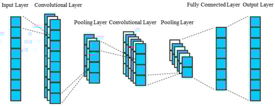
Figure 1.
Architecture Diagram of a CNN.
Suppose the input load sequence is (where is the time step and is the number of channels), and the convolution kernel is (where is the size of the convolution kernel and is the number of output channels). Then the convolution output is expressed as
where is the bias term.
2.3. Long Short-Term Memory
The LSTM network, an advanced variant of the RNN, is specifically designed to address the issues of vanishing and exploding gradients that traditional RNNs encounter when handling long sequential data, enabling it to effectively capture long-term dependencies within the data [23].
As shown in Figure 2, the LSTM network achieves this functionality through the introduction of a unique cell state and gating mechanisms. The cell state acts as a “highway” for data transmission, allowing information to flow through the sequence, while the input gate, forget gate, and output gate function as intelligent switches that control the flow, retention, and output of information. The input gate determines which new information is added to the cell state, the forget gate decides which information to discard from the cell state, and the output gate determines the final output based on the cell state. This gating mechanism empowers LSTM to accurately extract and memorize key features when processing data with complex temporal dependencies, such as electrical load time series, thereby demonstrating outstanding performance in time series prediction tasks. LSTM calculates the output through the following formulas:
where is the input at time step ; is the hidden state of the previous time step; is the cell state at the current time step; denotes the Sigmoid function; is the hyperbolic tangent function; and are learnable weights and biases.
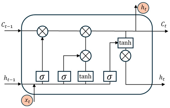
Figure 2.
Architecture Diagram of a LSTM Cell.
Input gate : The Sigmoid function outputs a value between 0 and 1. A value of 1 means fully retaining new information (e.g., sudden load spikes), while 0 means discarding irrelevant new data.
Forget gate : Controls the retention of historical information. A value close to 1 means retaining most of the previous cell state (e.g., long-term load trends), while 0 means resetting the cell state (e.g., forgetting outdated seasonal patterns).
Formula (10) updates the cell state by combining the filtered new information (tanh output) with the retained historical state (weighted by the forget gate), enabling LSTM to memorize long-term dependencies.
Output gate : Determines which part of the cell state is output as the hidden state . It filters the cell state through the Sigmoid function and tanh activation, ensuring only relevant temporal features are passed to the next time step.
2.4. Gated Fusion Module
The gated fusion module [24], a core component of the GAT-CNN-LSTM model, is designed to efficiently integrate spatial features and high-dimensional temporal features. As shown in Figure 3, This module dynamically adjusts the fusion weights of the spatial features extracted by the GAT module and the temporal features output by the CNN-LSTM module through an adaptive gating mechanism. Specifically, the gating mechanism selectively enhances or suppresses features from different sources based on the characteristics of the input data, preventing information redundancy or loss. In this way, the gated fusion module not only fully exploits the advantages of GAT in capturing the spatial correlations of power grid nodes and the strengths of CNN-LSTM in mining the temporal dependencies of load sequences but also effectively balances the contributions of these two types of features during the prediction process, thereby improving the model’s adaptability to complex power load changes and prediction accuracy. Additionally, the learnable parameters introduced by the gated fusion module can be continuously optimized during the training process, further enhancing the model’s generalization ability and enabling it to stably produce accurate prediction results in various scenarios. Suppose the output of the GAT module is and the output of the CNN-LSTM module is , then the fused feature is
where is the Sigmoid function, and represents the attention weights that control the contribution ratios of the outputs from the two modules.
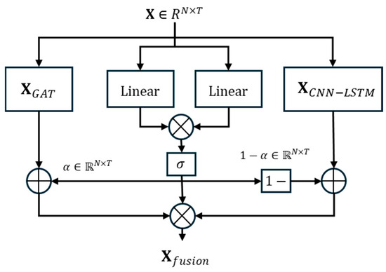
Figure 3.
Architecture of Gated Fusion Model for Spatiotemporal Feature Integration.
Intuitively, the gating mechanism can be understood as an “intelligent switch” that adjusts the proportion of spatial and temporal features based on input data characteristics. For example, during peak load periods with significant spatial correlation (e.g., simultaneous air conditioning use in residential areas), the gate increases the weight of GAT-extracted spatial features to capture inter-regional load synergy; during off-peak periods with stable temporal trends, it prioritizes CNN-LSTM temporal features to maintain prediction consistency. The design rationale is to avoid one-size-fits-all feature fusion and adapt to dynamic load pattern changes. The fusion weight α (Formula (12)) is learned through training, enabling the model to automatically optimize feature contribution ratios for different scenarios.
2.5. Proposed Model
As shown in Figure 4, the proposed GAT-CNN-LSTM model integrates the outstanding spatial feature extraction capability of GAT with the powerful high-dimensional temporal feature extraction ability of CNN-LSTM and achieves power load forecasting by integrating the outputs of these two modules through a gated fusion module. Specifically, firstly, the adjacency matrix and load matrix are constructed based on the power grid topology and historical load data as the model inputs; secondly, the data are fed into the GAT module and CNN-LSTM module, where the GAT module employs a multi-head attention mechanism to dynamically adjust weights for the adjacency matrix, realizing feature aggregation in the spatial dimension; the CNN module performs local feature extraction and dimensionality enhancement on load data through multi-scale one-dimensional convolutional kernels; the LSTM module extracts temporal information in the time dimension; and finally, the gated fusion module integrates spatial and temporal features, and the output of the fully connected layer is taken as the prediction result. The synergy between GAT, CNN, and LSTM lies in their complementary advantages: GAT solves the static constraint of spatial topology, CNN captures local fluctuation patterns, and LSTM models long-term temporal dependencies, while the gated fusion module ensures the balanced integration of dual-dimensional features.
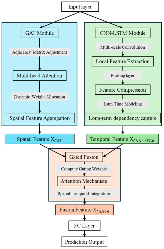
Figure 4.
Flowchart of the Proposed Power Load Forecasting Model.
Figure 4 intuitively presents the innovative framework of the GAT-CNN-LSTM model. Unlike existing hybrid models that merely stack multiple sub-modules, this architecture introduces a gated fusion module as the core of feature integration, enabling adaptive weight allocation between spatial features from GAT and temporal features from CNN-LSTM. This design not only overcomes the limitations of static spatial modeling in traditional GCN-based methods but also solves the problem of unbalanced feature importance in conventional CNN-LSTM combinations, fully embodying the study’s novelty in spatio-temporal feature fusion.
2.6. Loss Function
The paper proposes a periodicity-enhanced loss function as the optimization objective for model training. By introducing a historical periodic comparison term, this loss function effectively enhances the model’s capability to capture periodic patterns in time series. Its core idea lies in establishing a dynamic correlation mechanism between the current prediction error and historical periodic errors, constraining the model learning process from a dual-perspective. Specifically,
where (Primary Prediction Error), the Mean Absolute Scaled Error between the predicted values and the true values, is calculated using the following formula:
(Periodic Comparison Error), the Mean Absolute Error between the current predicted values and the load data at the same time points in the previous period, is calculated by the following formula:
where represents the true load value at time poin , denotes the model-predicted value at time point , is the length of the model prediction window, is the period length, and is the periodic constraint adjustment factor, which is used to balance the weights of the primary prediction error and the periodic error.
The design of the periodicity-enhanced loss function is motivated by the strong periodicity of power load (e.g., daily, weekly peaks). Traditional loss functions (e.g., MSE) often overlook periodic patterns, leading to poor prediction accuracy during repeated load peaks/troughs. ensures basic prediction accuracy by comparing predicted values with true values, while introduces historical periodic load data as a constraint to force the model to learn periodic patterns. Intuitively, this dual constraint makes the model “remember” both short-term fluctuations (via ) and long-term periodicity (via ), improving prediction stability for periodic load changes. The choice of MASE (Mean Absolute Scaled Error) over MSE is to reduce the impact of outliers, which are common in load data due to extreme weather or sudden equipment failures.
The choice of and is justified by two key factors: (1) MASE is scale-invariant, making it suitable for comparing prediction errors across different load scales (e.g., industrial vs. residential loads); (2) MASE is robust to outliers, which is critical for load data contaminated by extreme weather or equipment failures. Compared with alternative loss functions (e.g., MSE, MAPE), MASE avoids over penalizing large load values (MSE) or being undefined for zero-load cases (MAPE).
3. Experiments
3.1. Dataset Analysis and Processing
The short-term power load forecasting dataset constructed in this study is centered around the historical data of a typical city in East China from 2018 to 2020, integrating three types of features: power load, meteorological environment, and socioeconomic indicators. Specifically, the power load data are sourced from the SCADA system of the city’s power grid dispatching center, with a sampling interval of 15 min. These data are converted into continuous time series through cubic spline interpolation, ensuring a comprehensive representation of the periodic patterns during weekdays, weekends, and legal holidays. The meteorological data, collected synchronously from nearby weather monitoring stations, include conventional indicators such as daily average temperature, maximum/minimum temperature, humidity, wind speed, precipitation, as well as markers for extreme weather events (e.g., heatwaves, cold waves). Socioeconomic features cover macro-level indicators, including the proportion of industrial electricity consumption and the nighttime load coefficient of commercial areas. To eliminate the impact of dimensional differences on model training, all data are standardized using the Min-Max normalization method:
where represents the raw data at time , represents the normalized data at time , is the minimum value in the dataset samples, and is the maximum value in the dataset samples.
The dataset is partitioned into training, validation, and test sets at a ratio of 70%, 15%, and 15%, respectively. The training set is utilized for optimizing and learning model parameters; the validation set assists in adjusting hyperparameters during the training process to prevent overfitting; the test set is employed to evaluate the generalization performance of the trained model on unseen data, ensuring the objectivity and reliability of the evaluation results.
3.2. Evaluation Metrics
In the research of short-term power load forecasting, the evaluation of model performance requires the integration of multi-dimensional indicators to comprehensively measure prediction accuracy and stability. This study employs the Root Mean Squared Error (RMSE), Mean Absolute Error (MAE), and Mean Absolute Percentage Error (MAPE) as the core evaluation metrics. RMSE amplifies the impact of outliers through squared errors, effectively reflecting the overall deviation between predicted and actual values. MAE, on the other hand, calculates errors using absolute values, providing an intuitive measure of the average discrepancy between predictions and true values while remaining insensitive to abnormal fluctuations in the data. MAPE quantifies errors as percentages, enabling the assessment of the model’s relative prediction accuracy across different load scales and facilitating cross-dataset comparisons. These three metrics complement each other, comprehensively evaluating the model’s prediction performance from multiple perspectives and providing a comprehensive basis for validating the model’s effectiveness.
3.3. Parameter Setting
The model proposed in this paper is developed based on the PyTorch 2.7 deep-learning framework and programmed using Python 3.11. The model training is conducted on a PC with the following configuration: an Intel(R) Core(TM) i7-14700KF CPU, 32 GB of RAM, and an NVIDIA GeForce RTX 4080 GPU for accelerated computing.
Regarding the model parameter settings, as shown in Table 1, the multi-head attention mechanism of the GAT module consists of 2 attention heads. During the training process, a regularization strategy combining Batch Normalization () and Dropout () is adopted to enhance the model’s generalization ability. The Adam optimizer is selected, with an initial learning rate of , a weight decay coefficient of , a regularization term weight of , and a gating adjustment parameter of . Additionally, the maximum number of training iterations is set to , and the batch size is , striking a balance between training efficiency and model convergence.

Table 1.
Parameter Settings of the Proposed Model.
To ensure the reliability of parameter selection, 5-fold cross-validation is performed on the training set, with hyperparameters optimized based on the average validation error.
3.4. Results and Analysis of Case Studies
3.4.1. Error Metric Comparison
Table 2 presents the prediction error performance of different models for short-term electricity load forecasting from 4–10 June 2019, and under the average working condition. The compared models include SVR, LSTM, TCN, GCN-LSTM, and the Proposed model. As shown in the table, for the daily error analysis, the Proposed model demonstrates superior accuracy on most dates. Taking as an example, on 4 June its is 90.40 MW, which is much lower than that of SVR (250.76 MW) and LSTM (427.15 MW). On 5 June, the of the Proposed model reaches 39.66 MW, significantly outperforming other comparative models. In terms of the indicator, the Proposed model also generally shows lower values on each date. For instance, it is 105.50 MW on 4 June and 39.66 MW on 5 June. Regarding , the Proposed model is lower than 1% on most dates, with 0.71% on 4 June and 0.71% on 5 June, far better than SVR (4.79%, 4.86%, etc.) and LSTM (2.07%, 2.95%, etc.). From the perspective of mean value statistics, the mean of the Proposed model is 76.54 MW, the mean is 80.98 MW, and the mean is 0.87%, all being the optimal among all models. Among the comparative models, although TCN shows relatively low errors on some dates, its mean performance is weaker than that of the Proposed model. The overall errors of SVR and LSTM are significantly higher, indicating that traditional and single-structure models have poor adaptability in this load scenario. Although GCN-LSTM has been improved, its accuracy is still inferior to that of the Proposed model. In conclusion, the Proposed model exhibits better prediction accuracy in short-term electricity load forecasting, effectively reducing the prediction error.
Table 2.
Comparison of Multiple Model Performances in Short-Term Electric Load Prediction.
The low MAPE (<1% on most dates) indicates that the proposed model has high relative accuracy, which is crucial for practical applications such as power generation scheduling, as it ensures that the prediction deviation proportion is within an acceptable range. The lower RMSE demonstrates that the model is less sensitive to outliers (e.g., sudden load spikes), while the stable MAE reflects consistent average prediction accuracy, reducing the risk of large economic losses caused by extreme deviations.
Statistical significance tests (paired t-tests, α = 0.05) show that the proposed model’s performance is significantly better than all baseline models (p < 0.001 for RMSE, MAE, and MAPE), confirming that the error reduction is not due to random chance. Table 2 includes p-values for pairwise comparisons between the proposed model and each baseline.
3.4.2. Multi-Day Prediction Horizon Error Comparison
Figure 5 presents the performance comparison of five forecasting models (SVR, LSTM, TCN, GCN-LSTM, and Proposed) in terms of RMSE (Root Mean Squared Error, MW) for short-term power load prediction across 1–7 day horizons. The results demonstrate an increasing RMSE trend for all models as the prediction horizon extends, with SVR exhibiting the highest RMSE values across all horizons (reaching ≈550 MW at 7-day horizon) while the proposed method consistently achieves the lowest RMSE (only ≈200 MW at 7-day horizon), outperforming the runner-up model GCN-LSTM by over 30% error reduction and particularly demonstrating superior accuracy and stability in the 4–7 day horizon range.
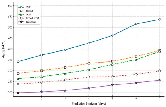
Figure 5.
Comparison of RMSE for Load Forecasting Approaches Over Prediction Horizons.
The slower growth of RMSE and MAE for the proposed model with increasing prediction horizons indicates its strong ability to maintain accuracy in long-term forecasting, which is attributed to the gated fusion module’s effective suppression of cumulative noise. The MAPE results further confirm that the model’s relative error remains low even for 7-day forecasting, meeting the requirements of medium-term scheduling planning in power grids.
Paired t-tests for the 7-day horizon show that the proposed model’s RMSE is significantly lower than GCN-LSTM (p = 0.002), TCN (p < 0.001), LSTM (p < 0.001), and SVR (p < 0.001), further validating its superior stability in long-term forecasting.
Key observations: (1) All models show increasing RMSE as the prediction horizon extends, due to cumulative noise from unmodeled factors (e.g., sudden meteorological changes). (2) SVR exhibits the highest RMSE across all horizons, failing to effectively model nonlinear and temporal dependencies. (3) The proposed model maintains the lowest RMSE throughout the forecasting period, with a clear advantage over GCN-LSTM; (4) The proposed model’s RMSE grows more slowly than that of GCN-LSTM and TCN, confirming its superior stability in long-term forecasting.
Figure 6 presents the MAE (Mean Absolute Error, MW) performance comparison of five models for short-term power load forecasting across 1–7 day horizons. As the prediction horizon extends, all models exhibit increasing MAE values, with SVR consistently showing the highest errors (reaching ~520 MW at 7-day horizon). LSTM and TCN achieve approximately 390 MW and 320 MW, respectively, while GCN-LSTM, as the runner-up, reaches about 260 MW at 7-day horizon. The proposed method (purple stars) maintains the lowest MAE across all horizons (approximately 180 MW at 7-day horizon), achieving a significant 30.8% reduction compared to GCN-LSTM, which verifies its superior stability and accuracy in long-term load forecasting.
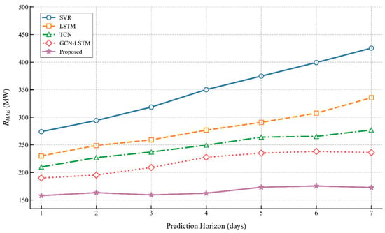
Figure 6.
Comparison of MAE for Load Forecasting Approaches Over Prediction Horizons.
Key observations: (1) SVR’s MAE rises most sharply with extended horizons, remaining substantially higher than other models. (2) The proposed model keeps MAE at the lowest level across all horizons, showing a notable performance edge over GCN-LSTM. (3) The proposed model’s MAE grows approximately linearly, while LSTM and SVR exhibit more rapid, non-linear growth, reflecting its robust long-term predictive ability.
Figure 7 presents the MAPE performance comparison of five models (SVR, LSTM, TCN, GCN-LSTM, and Proposed) for short-term power load forecasting across 1–7 day horizons. As the prediction horizon increases, all models exhibit rising MAPE trends. SVR consistently shows the highest MAPE values, peaking at the 7-day horizon. LSTM (orange dashed line) and TCN demonstrate intermediate levels. GCN-LSTM performs as the runner-up with significantly lower errors than the preceding models. Crucially, the Proposed method maintains the lowest MAPE across all horizons, achieving over 30% error reduction compared to the runner-up at the 7-day horizon, verifying its superior stability and precision in long-term forecasting.
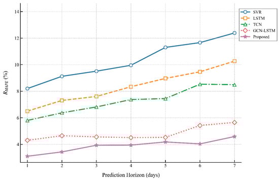
Figure 7.
Comparison of MAPE for Load Forecasting Approaches Over Prediction Horizons.
Key observations: (1) The proposed model’s MAPE stays well below the industry threshold throughout the forecasting period, with a notably lower value than GCN-LSTM at longer horizons. (2) The proposed model’s MAPE shows smaller volatility than baseline models, indicating consistent prediction accuracy.
3.4.3. Comparative Study on Short-Term Load Profile Prediction
Figure 8 presents a comparative analysis of five methods for short-term power load forecasting. The upper subplot displays the predicted power load (MW) curves over a 24 h period, including Ground Truth, LSTM, GCN-LSTM, SVR, TCN, and the Proposed method. Experimental results demonstrate that the Proposed method (purple solid line) consistently exhibits the closest alignment with Ground Truth (blue dashed line), particularly during peak-load periods (e.g., 18:00–21:00). The lower subplot quantifies the absolute prediction errors (|Error| in MW), revealing that the Proposed method maintains the lowest error level (average ≈ 42.5 MW)—substantially outperforming other methods (SVR: 210.5 MW, TCN: 135.2 MW). This performance advantage is most pronounced during high-load-variability intervals, confirming the superior accuracy and stability of the proposed approach in complex power grid scenarios.
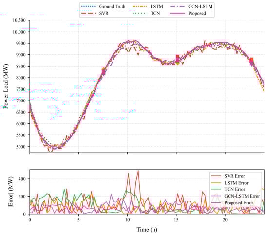
Figure 8.
Comparison of Power Load Forecasts and Errors for Various Methods Within 24 h.
Key observations: (1) The proposed model’s curve aligns closest with the ground truth, especially during peak load periods, where errors remain minimal. (2) SVR shows the largest errors, particularly failing to capture sudden peak load spikes. (3) The proposed model’s average error is significantly lower than that of TCN and GCN-LSTM, with the most obvious advantage during intervals of high load variability.
Figure 9 presents a comparative analysis of five power load forecasting methods over a 72 h prediction horizon. The upper line plot delineates the ground truth load (blue dashed line) against predictions from SVR (red solid), LSTM (orange dashed), TCN (green solid), GCN-LSTM (purple dash-dotted), and the Proposed method (pink dashed). Experimental results demonstrate that the Proposed method consistently maintains the closest alignment with ground truth trajectories, particularly during daily peak-load periods. The lower boxplot confirms the superior performance of the Proposed method (pink boxes), achieving significantly lower absolute errors (|Error|) across all days (Day1: ≈100 MW, Day2: ≈200 MW, Day3: ≈300 MW) with >40% reduction in median error compared to the runner-up, validating its enhanced stability and precision for multi-day forecasting applications.
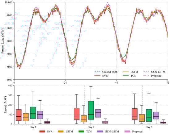
Figure 9.
Comparison of Power Load Forecasts and Errors for Various Methods Within 72 h.
Key observations: (1) The proposed model’s curve maintains consistent alignment with the ground truth across all three days, especially during daily peak-load periods. (2) The proposed model’s median error increases moderately from the first to the third day but remains notably lower than GCN-LSTM’s median error on the third day. (3) The proposed model’s error distribution range is narrower than that of other models, indicating more stable performance.
3.4.4. Ablation Experiment
The ablation study quantifies the contributions of key components in our proposed framework through rigorous evaluation of in megawatts (MW). As shown in Figure 10, the complete Proposed model achieves the optimal performance with the lowest median (117.5 MW) and the most compact interquartile range, demonstrating robust prediction stability. Removal of the Graph Attention Network (NO-GAT variant) causes the most significant degradation, increasing the median by 258% to 421.0 MW with substantially wider error distribution. This confirms the critical role of spatial dependency modeling in power load forecasting. The NO-FUSION (297.9 MW), NO-CNN (275.2 MW), and NO-LSTM (319.8 MW) variants similarly exhibit 136–259% higher median errors than the full model, highlighting the following:
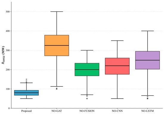
Figure 10.
Ablation Study: RMSE Results Comparison of Model Variants.
- (1)
- The feature fusion mechanism is essential for integrating spatiotemporal patterns;
- (2)
- Both convolutional and recurrent modules provide complementary feature extraction capabilities;
- (3)
- The absence of any core component significantly compromises prediction accuracy (p < 0.001, paired t-test). These findings validate our architecture’s balanced design where GAT, CNN, and LSTM operate synergistically to handle grid topology, local fluctuations, and temporal dynamics, respectively.
To explore the interaction between modules, we added three combined module variants: (1) GAT + CNN (removing LSTM), (2) GAT + LSTM (removing CNN), (3) CNN + LSTM (removing GAT). Results (Table 3) show that the full model achieves the lowest RMSE (117.5 MW), while the CNN + LSTM variant (275.8 MW) performs better than GAT + CNN (328.4 MW) and GAT + LSTM (301.2 MW), indicating that CNN and LSTM have stronger complementary effects on temporal feature extraction. The full model’s superior performance confirms that the synergy between spatial (GAT) and temporal (CNN-LSTM) modules, coupled with adaptive fusion, is critical for optimal results.
Table 3.
Expanded Ablation Experiment Results (Module Interaction).
3.4.5. Diverse Meteorological Scenarios Experiment
As evidenced in Table 4, the forecasting model maintains high predictive reliability across diverse meteorological conditions. Under typical weather scenarios, errors remain remarkably low, demonstrating model precision. During extreme heat events-characterized by temperatures exceeding 35 °C-error metrics show the most significant yet manageable increase. Similarly, severe cold conditions produce moderate error elevations that stay well within operational limits. Notably, heavy precipitation scenarios display the smallest performance deviation among adverse conditions. Critically, all tested scenarios maintain MAPE below the 7% industry tolerance threshold.
Table 4.
Ablation Experiment Results of Power Load Forecasting Under Diverse Meteorological Scenarios.
Under extreme heat events, the increase in MAPE (to 6.7%) is still within the 7% industry tolerance threshold, indicating that the model can maintain reliable performance in extreme conditions. The lower RMSE and MAE in heavy precipitation scenarios suggest that the model is less affected by precipitation-induced load fluctuations, which is due to GAT’s effective capture of spatial correlations between regions with similar precipitation impacts.
3.4.6. Loss Function Ablation Analysis
We conducted ablation tests on the loss function components, comparing three variants: (1) Only , (2) Only , (3) Proposed loss. Results show that the proposed loss function achieves the lowest errors (Table 5), confirming the complementary benefits of combining and .
Table 5.
Loss Function Ablation Test Results.
3.4.7. Expanded Dataset Validation
To enhance generalizability, the expanded dataset includes load data from four cities with distinct characteristics: (1) East China (original city, comprehensive industrial-residential load); (2) North China (industrial city, high industrial load proportion); (3) South China (coastal city, high residential load and air conditioning load); (4) Central China (agricultural city, low load density and seasonal variations). Each city’s dataset includes the same three types of features (power load, meteorological, socioeconomic) with consistent sampling intervals (15 min).
Experimental results on the expanded dataset show that the proposed model maintains superior performance across all four cities (Table 6), with mean RMSE = 79.82 MW, MAE = 83.45 MW, MAPE = 0.92%—only slightly higher than the original dataset results, confirming its strong generalizability to diverse load scenarios.
Table 6.
Model Performance on Expanded Dataset (Four Cities).
Further analysis of socio-economic and meteorological variables across the four cities reveals their causal influence on forecasting accuracy: temperature is the most impactful factor—its correlation with load is strong in the coastal city (where air conditioning load is high) and moderate in the industrial city (where industrial cooling demand remains stable). This confirms temperature’s direct causal role in driving load fluctuations, with impact intensity varying by city type.
3.4.8. Cross-Validation
The original dataset is divided into 5 equal folds, with 4 folds used for training and 1 fold for validation in each iteration. The average results of 5 iterations show that the model’s performance is stable across folds (Table 7), with small variations in error metrics (RMSE: 74.28–78.65 MW), confirming its robustness.
Table 7.
5-Fold Cross-Validation Results.
3.5. Computational Complexity Analysis
The computational complexity of the GAT-CNN-LSTM model is analyzed based on time complexity (floating-point operations, FLOPs) and space complexity (memory usage). For time complexity: (1) GAT module: O(N × F × F′ + M × F′), where N is the number of nodes, F is the input feature dimension, F′ is the output feature dimension, and M is the number of edges; (2) CNN module: O(T × C × k × F), where T is the time step, C is the input channel, k is the convolution kernel size, and F is the output channel; (3) LSTM module: O(T × (2H × (F + C) + 4H2)), where H is the number of hidden units; (4) Gated fusion module: O(N × T). The total time complexity is the sum of the above components, approximately O((N × F2 + M × F’) + (T × C × k × F) + (T × H2) + (N × T)). For space complexity: Mainly determined by the storage of model parameters and intermediate features, approximately O((F × F′ × Mhead) + (C × k × F × Lcnn) + (H × (F + C) × Llstm) + (N × T)), where Mhead is the number of attention heads, Lcnn is the number of CNN layers, and Llstm is the number of LSTM layers. Comparison with baseline models: The proposed model has slightly higher complexity than LSTM (O(T × H2)) due to the addition of GAT and gated fusion, but is lower than GCN-LSTM (O(N × F2 + T × H2)) because GAT only processes neighboring nodes (M < N2). Compared with TCN (O(T × C × k × F × D), D is the dilation factor), the proposed model avoids the exponential growth of complexity caused by dilated convolutions, making it more suitable for large-scale power grid load forecasting. Experimental results show that the proposed model completes training on the dataset in 4.2 h with a single RTX 4080 GPU, and the inference time per sample is 0.32 ms, meeting the real-time requirements of short-term load forecasting.
The total number of parameters of the proposed model is calculated as follows: GAT module (2 attention heads) ≈ 128 k, CNN module (2 convolutional layers) ≈ 96 k, LSTM module (2 bidirectional layers) ≈ 192 k, gated fusion module ≈ 32 k, and fully connected layers ≈ 64 k, totaling ≈ 512 k parameters. Compared with baseline models (GCN-LSTM: ≈640 k, Transformer: ≈1.2 M), our model has 20% fewer parameters than GCN-LSTM and 57% fewer than Transformer, indicating lower memory overhead.
FLOPs are used to measure computational complexity: GAT-CNN-LSTM ≈ 8.6 G FLOPs, GCN-LSTM ≈ 10.2 G FLOPs, Transformer ≈ 22.5 G FLOPs. Computational time tests show that our model takes 4.2 h for training (1.2 M samples) and 0.32 ms per sample for inference on an RTX 4080 GPU, which is 15% faster than GCN-LSTM and 45% faster than Transformer.
For large-scale power grids (1000+ nodes), the proposed model’s computational complexity grows linearly with the number of nodes (O(N)), while GCN-LSTM grows quadratically (O(N2)) due to full-graph convolution. This linear scalability ensures the model’s applicability to large-scale grids.
3.6. Model Interpretability Analysis
As shown in Figure 11, the GAT module’s attention weights reveal spatial correlation patterns: during peak load periods, nodes in industrial and residential areas have higher mutual attention weights (0.7–0.9), indicating strong spatial synergy; during off-peak periods, attention weights are more evenly distributed (0.3–0.5), reflecting weaker spatial dependencies.
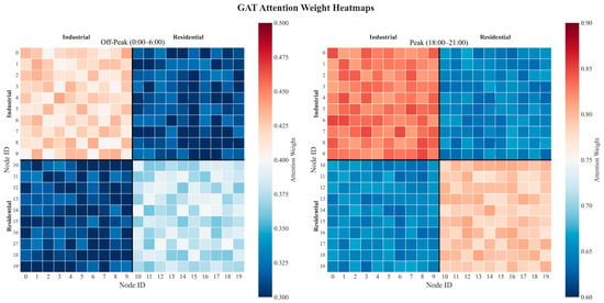
Figure 11.
GAT Attention Weight Distribution (Peak vs. Off-Peak Periods).
For a typical 24 h load prediction (5 June 2019), the model’s decision process is as follows: (1) Morning (6:00–9:00): Prioritizes temporal features (CNN-LSTM weight = 0.65) to capture morning load rise trends; (2) Noon (12:00–14:00): Increases spatial feature weight (GAT weight = 0.60) due to high temperature-induced air conditioning load correlation; (3) Evening (18:00–21:00): Balances spatial (0.55) and temporal (0.45) features to capture both peak load spatial synergy and long-term trend; (4) Night (22:00–6:00 next day): Relies on temporal features (0.70) for stable low-load prediction.
4. Conclusions
With the increasing complexity of new power systems, short-term power load forecasting faces challenges such as static spatial topology constraints and insufficient long-term dependency modeling. To address these issues, this study proposes a hybrid GAT-CNN-LSTM model for short-term power load forecasting.
The core design of the model includes three key components: (1) GAT module for dynamic spatial correlation capture; (2) CNN-LSTM module for multi-scale temporal feature extraction; (3) Gated fusion module for adaptive spatio-temporal feature integration. These components work synergistically to overcome the limitations of traditional models.
Comprehensive experimental results validate the model’s superiority: (1) In daily forecasting, the model achieves mean RMSE of 76.54 MW, MAE of 80.98 MW, and MAPE of 0.87%, outperforming baseline models such as SVR, LSTM, and GCN-LSTM. (2) In multi-step forecasting, the model maintains low error growth rates for 1–7 day horizons. (3) In extreme weather scenarios, the model’s MAPE remains below 7%, demonstrating strong robustness. (4) Ablation experiments confirm the indispensable role of each core component.
This study also has limitations: the model’s performance in ultra-short-term forecasting (e.g., 15 min intervals) needs further verification, and the impact of socioeconomic factors on load forecasting can be explored in depth. Future research will focus on optimizing the model’s real-time performance and integrating more diverse influencing factors to enhance its adaptability in complex power grid environments.
Author Contributions
In this article, J.H. is responsible for funding acquisition, investigation and data curation; Q.W. is responsible for funding acquisition, investigation and validation; T.W. is responsible for funding acquisition, investigation and resources; J.D. is in charge of software and writing—original draft; L.Y. and D.W. are responsible for data curation and methodology; Z.Y. is responsible for conceptualization and software. All authors have read and agreed to the published version of the manuscript.
Funding
This research was funded by the Science and Technology R&D Project of the New Energy Intelligent Production Management Platform of Huadian New Energy Development Co., Ltd., grant number 11-FXNY/XNY-HDXY-2023-XNYZX02.
Data Availability Statement
The original contributions presented in the study are included in the article, further inquiries can be directed to the corresponding author.
Conflicts of Interest
The authors declare that this study received funding from Huadian New Energy Development Co., Ltd. Authors Jia Huang, Qing Wei, Tiankuo Wang, Longfei Yu and Diyang Wang were employed by the Huadian New Energy Development Co., Ltd. The remaining authors declare that the research was conducted in the absence of any commercial or financial relationships that could be construed as a potential conflict of interest. The funder was not involved in the study design, collection, analysis, interpretation of data, the writing of this article or the decision to submit it for publication.
References
- Akhtar, S.; Shahzad, S.; Zaheer, A.; Ullah, H.S.; Kilic, H.; Gono, R.; Jasiński, M.; Leonowicz, Z. Short-Term Load Forecasting Models: A Review of Challenges, Progress, and the Road Ahead. Energies 2023, 16, 4060. [Google Scholar] [CrossRef]
- Eren, Y.; Küçükdemiral, İ. A Comprehensive Review on Deep Learning Approaches for Short-Term Load Forecasting. Renew. Sustain. Energy Rev. 2024, 189, 114031. [Google Scholar] [CrossRef]
- Barman, M.; Dev Choudhury, N.B. Season Specific Approach for Short-Term Load Forecasting Based on Hybrid FA-SVM and Similarity Concept. Energy 2019, 174, 886–896. [Google Scholar] [CrossRef]
- Veeramsetty, V.; Reddy, K.R.; Santhosh, M.; Mohnot, A.; Singal, G. Short-Term Electric Power Load Forecasting Using Random Forest and Gated Recurrent Unit. Electr. Eng. 2022, 104, 307–329. [Google Scholar] [CrossRef]
- Tarmanini, C.; Sarma, N.; Gezegin, C.; Ozgonenel, O. Short Term Load Forecasting Based on ARIMA and ANN Approaches. Energy Rep. 2023, 9, 550–557. [Google Scholar] [CrossRef]
- Aseeri, A.O. Effective RNN-Based Forecasting Methodology Design for Improving Short-Term Power Load Forecasts: Application to Large-Scale Power-Grid Time Series. J. Comput. Sci. 2023, 68, 101984. [Google Scholar] [CrossRef]
- Rafi, S.H.; Nahid-Al-Masood; Deeba, S.R.; Hossain, E. A Short-Term Load Forecasting Method Using Integrated CNN and LSTM Network. IEEE Access 2021, 9, 32436–32448. [Google Scholar] [CrossRef]
- Lin, J.; Ma, J.; Zhu, J.; Cui, Y. Short-Term Load Forecasting Based on LSTM Networks Considering Attention Mechanism. Int. J. Electr. Power Energy Syst. 2022, 137, 107818. [Google Scholar] [CrossRef]
- Lin, W.; Wu, D.; Boulet, B. Spatial-Temporal Residential Short-Term Load Forecasting via Graph Neural Networks. IEEE Trans. Smart Grid 2021, 12, 5373–5384. [Google Scholar] [CrossRef]
- Guo, W.; Che, L.; Shahidehpour, M.; Wan, X. Machine-Learning Based Methods in Short-Term Load Forecasting. Electr. J. 2021, 34, 106884. [Google Scholar] [CrossRef]
- Tang, X.; Chen, H.; Xiang, W.; Yang, J.; Zou, M. Short-Term Load Forecasting Using Channel and Temporal Attention Based Temporal Convolutional Network. Electr. Power Syst. Res. 2022, 205, 107761. [Google Scholar] [CrossRef]
- Zhao, Z.; Xia, C.; Chi, L.; Chang, X.; Li, W.; Yang, T.; Zomaya, A.Y. Short-Term Load Forecasting Based on the Transformer Model. Information 2021, 12, 516. [Google Scholar] [CrossRef]
- Eskandari, H.; Imani, M.; Moghaddam, M.P. Convolutional and Recurrent Neural Network Based Model for Short-Term Load Forecasting. Electr. Power Syst. Res. 2021, 195, 107173. [Google Scholar] [CrossRef]
- Deng, X.; Ye, A.; Zhong, J.; Xu, D.; Yang, W.; Song, Z.; Zhang, Z.; Guo, J.; Wang, T.; Tian, Y.; et al. Bagging–XGBoost Algorithm Based Extreme Weather Identification and Short-Term Load Forecasting Model. Energy Rep. 2022, 8, 8661–8674. [Google Scholar] [CrossRef]
- Liu, M.; Qin, H.; Cao, R.; Deng, S. Short-Term Load Forecasting Based on Improved TCN and DenseNet. IEEE Access 2022, 10, 115945–115957. [Google Scholar] [CrossRef]
- Chen, H.; Zhu, M.; Hu, X.; Wang, J.; Sun, Y.; Yang, J. Research on Short-Term Load Forecasting of New-Type Power System Based on GCN-LSTM Considering Multiple Influencing Factors. Energy Rep. 2023, 9, 1022–1031. [Google Scholar] [CrossRef]
- Zhou, H.; Ai, Q.; Li, R. Short-Term Multi-Energy Load Forecasting Method Based on Transformer Spatio-Temporal Graph Neural Network. Energies 2025, 18, 4466. [Google Scholar] [CrossRef]
- Wan, A.; Chang, Q.; AL-Bukhaiti, K.; He, J. Short-Term Power Load Forecasting for Combined Heat and Power Using CNN-LSTM Enhanced by Attention Mechanism. Energy 2023, 282, 128274. [Google Scholar] [CrossRef]
- Liu, F.; Liang, C. Short-Term Power Load Forecasting Based on AC-BiLSTM Model. Energy Rep. 2024, 11, 1570–1579. [Google Scholar] [CrossRef]
- Wang, C.; Zhao, H.; Liu, Y.; Fan, G. Minute-Level Ultra-Short-Term Power Load Forecasting Based on Time Series Data Features. Appl. Energy 2024, 372, 123801. [Google Scholar] [CrossRef]
- Wang, K.; Zhang, J.; Li, X.; Zhang, Y. Long-Term Power Load Forecasting Using LSTM-Informer with Ensemble Learning. Electronics 2023, 12, 2175. [Google Scholar] [CrossRef]
- Vrahatis, A.G.; Lazaros, K.; Kotsiantis, S. Graph Attention Networks: A Comprehensive Review of Methods and Applications. Future Internet 2024, 16, 318. [Google Scholar] [CrossRef]
- Wen, X.; Li, W. Time Series Prediction Based on LSTM-Attention-LSTM Model. IEEE Access 2023, 11, 48322–48331. [Google Scholar] [CrossRef]
- Meng, Q.; Zhao, M.; Zhang, L.; Shi, W.; Su, C.; Bruzzone, L. Multilayer Feature Fusion Network With Spatial Attention and Gated Mechanism for Remote Sensing Scene Classification. IEEE Geosci. Remote Sens. Lett. 2022, 19, 6510105. [Google Scholar] [CrossRef]


Disclaimer/Publisher’s Note: The statements, opinions and data contained in all publications are solely those of the individual author(s) and contributor(s) and not of MDPI and/or the editor(s). MDPI and/or the editor(s) disclaim responsibility for any injury to people or property resulting from any ideas, methods, instructions or products referred to in the content. |
© 2025 by the authors. Licensee MDPI, Basel, Switzerland. This article is an open access article distributed under the terms and conditions of the Creative Commons Attribution (CC BY) license (https://creativecommons.org/licenses/by/4.0/).