Abstract
To address the problems of local optima and insufficient convergence accuracy in parameter identification of primary frequency regulation (PFR) for steam turbines, this paper proposed a hybrid identification method that integrated an Improved Bayesian Optimization (IBO) algorithm and an Improved Whale Optimization Algorithm (IWOA). By initializing the Bayesian parameter population using Tent chaotic mapping and the reverse learning strategy, employing a radial basis kernel function hyperparameter training mechanism based on the Adam optimizer and optimizing the Expected Improvement (EI) function using the Limited-memory Broyden–Fletcher– Goldfarb–Shanno with Bounds (L-BFGS-B) method, IBO was proposed to obtain the optimal candidate set with the smallest objective function value. By introducing a nonlinear convergence factor and the adaptive Levy flight perturbation strategy, IWOA was proposed to obtain locally optimized optimal solutions. By using the reverse-guided optimization mechanism and employing a fitness-oriented selection strategy, the optimal solution was chosen to complete the closed-loop process of reverse learning feedback. Nine standard test functions and the Proportional Integral Derivative (PID) parameter identification of the electro-hydraulic servo system in a 330 MW steam turbine were presented as examples. Compared with Particle Swarm Optimization (PSO), Whale Optimization Algorithm (WOA), Bayesian Optimization (BO) and Particle Swarm Optimization-Grey Wolf Optimizer (PSO-GWO), the Improved Bayesian Optimization-Whale Optimization Algorithm (IBO-WOA) proposed in this paper has been validated to effectively avoid the problem of getting stuck in local optima during complex optimization and has high parameter recognition accuracy. Meanwhile, an Out-Of-Distribution (OOD) Test based on noise injection had demonstrated that IBO-WOA had good robustness. The time constant identification of the steam turbine were carried out using IBO-WOA under two experimental conditions, and the identification results were input into the PFR model. The simulated power curve can track the experimental measured curve well, proving that the parameter identification results obtained by IBO-WOA have high accuracy and can be used for the modeling and response characteristic analysis of the steam turbine PFR.
1. Introduction
Thermal power units undertake the primary frequency regulation (PFR) tasks in the power system. In order to accurately analyze the dynamic response characteristics of PFR and optimize control performance, it is essential to construct a high-precision PFR model, with accurate parameter identification being the key prerequisite [1]. The dynamic parameter identification of the Digital Electro-Hydraulic (DEH) system directly determines the speed, amplitude, and stability of a unit response to load commands and grid frequency disturbances, thereby significantly affecting the overall PFR performance of the system [2]. Therefore, the development of a high-precision and robust parameter identification method is of great significance for improving the PFR performance of a steam turbine and even the stability level of the whole power grid.
Essentially, parameter identification is a multidimensional function optimization problem, aiming to find a parameter set that enables the model output to best fit the actual dynamic data. Commonly used parameter identification methods include deterministic algorithms and heuristic intelligent optimization methods. Deterministic methods such as gradient descent method [3], least squares method [4], usually demonstrate high computational efficiency and fast convergence. However, their identification results heavily rely on the initial guess value and require strict continuity and differentiability of the objective function. In the context of nonlinear and complex power systems with multiple local minima, these approaches are prone to falling into local optima, making it difficult to guarantee global performance. To overcome these limitations, heuristic intelligent optimization methods have been widely adopted in the field of complex system identification due to their independence from gradient information and good global search ability. Representative algorithms include Particle Swarm Optimization (PSO) [5], Genetic Algorithms (GA) [6], Simulated Annealing (SA) [7], Grey Wolf Optimizer (GWO) [8], Whale Optimization Algorithm (WOA) [9], and Bayesian Optimization (BO) [10]. These algorithms each have their own advantages and disadvantages: PSO converges quickly but tends to premature convergence; GA excels in global exploration but lacks local refinement ability; WOA has gained attention for its simple structure and strong local search ability but still suffers from premature convergence and insufficient global exploration. In general, a single intelligent optimization algorithm faces common challenges in complex system parameter identification, such as balancing exploration and utilization ability, improving convergence accuracy and speed, and avoiding getting stuck in local optima.
In recent years, BO and WOA have gained widespread application in heuristic intelligent optimization methods. Boasting strong learning capabilities for unknown functions and efficient objective-oriented optimization mechanisms, BO demonstrates unique advantages in parameter optimization problems. By constructing probabilistic proxy models of the most promising regions and selecting next evaluation points through function acquisition, it effectively reduces the number of function evaluations. Some studies have attempted to apply BO to state estimation in power systems or optimization of specific component parameters, achieving certain results. Using BO, Xu, Y optimized synchronous generator excitation system parameters to improve state estimation accuracy [10]. Tang, M.N. took a 5 MW horizontal axis wind turbine as the research object and proposed a parameter adaptive robust control method, which achieved self-optimization of controller parameters through Bayesian optimization [11]. However, when addressing high-dimensional global parameter joint identification problems involving strong nonlinear dynamics, the standard Gaussian process (GP) model exhibits limitations. The selection of GP kernel functions and hyperparameter optimization significantly impacts performance, potentially leading to excessive smoothing of the objective function’s dynamics, making it difficult to accurately capture nonlinear characteristics. When the objective function exhibits multiple local optima or excessive noise due to strong nonlinearity or measurement noise interference, the search direction of BO may be misled and fall into suboptimal solutions, making it difficult to achieve true global optimal parameter identification. As an efficient swarm intelligence algorithm, WOA demonstrates remarkable convergence speed, particularly excelling in moderately dimensioned problems. Based on WOA, Shaheen proposed a Vehicle-to-Grid (V2G) scheduling model and a fair and economical Distributed Energy Resource (DER) allocation scheme based on Game Theory (GT), thus constructing a new dual layer energy management system (EMS) framework that provides a comprehensive solution for sustainable Autonomous Microgrids management [12]. Li, Y.T used WOA to analyze the parameters of the inverter control system that dominates the output characteristics of the double-fed induction generator (DFIG) in dynamic full process simulation and establishes a detailed dynamic model of DFIG with inverters. The results showed that WOA can identify control system parameters faster and more accurately [13]. However, when addressing high dimensional Proportional Integral Derivative (PID) parameter identification in a steam turbine, the stochastic characteristics of WOA in initialization and population search strategies make it prone to premature convergence and local optimization, especially when the global structure of the identification space remains unclear.
To address the limitations of single algorithms, researchers have proposed various improvement strategies. On the one hand, they aim to enhance the optimization performance of a single algorithm. More importantly, the improvement direction is to combine the advantages of different algorithms and adopt hybrid optimization methods, such as PSO and GA hybrid [14], GWO and WOA hybrid [15,16], BO and GA hybrid [17], etc. to use the complementarity of different algorithms to cover the solution space and improve performance identification accuracy. Confronting challenges in PFR parameter identification for a steam turbine, particularly the vulnerability of existing heuristic optimization algorithms to global exploration failures and local minima trapping, this study proposes a hybrid identification method combining Improved Bayesian Optimization (IBO) with Improved Whale Optimization Algorithm (IWOA) to achieve the identification of PFR parameters for a steam turbine. The innovations of this paper are as follows: (1) By initializing the Bayesian parameter population using Tent chaotic mapping and the reverse learning strategy, employing a radial basis kernel function hyperparameter training mechanism based on the Adam optimizer, and optimizing the Expected Improvement (EI) function using the Limited-memory Broyden–Fletcher–Goldfarb–Shanno with Bounds (L-BFGS-B) method, IBO was proposed. It can overcome the shortcomings of strong locality and low exploration efficiency during population initialization and solve the problem of low efficiency in optimizing key hyperparameters using traditional methods. (2) By introducing a nonlinear convergence factor and the adaptive Levy flight perturbation strategy, IWOA was proposed which can overcome the drawback of WOA being prone to getting stuck in local optima and further enhance the local search capability of WOA. (3) For the first time, we deeply integrate IBO with IWOA, utilizing the reverse-guided optimization mechanism to construct a three-layer collaborative architecture: “Bayesian global guidance-WOA local optimization-reverse learning feedback.” This significantly improves global search capability and convergence speed during parameter identification, achieving high precision and robustness.
To validate the feasibility and superiority of our method, simulations were conducted on nine standard test functions and PID parameter identification case for the electro-hydraulic servo systems, compared with PSO, WOA, BO, and PSO-GWO algorithms. Experimental verification was performed on a steam turbine volumetric time constant identification and applied to the PFR simulation modeling and analysis. The analysis results indicate that Improved Bayesian Optimization-Whale Optimization Algorithm (IBO-WOA) had better global search ability, local optimal area escape ability and robustness, and its identification results had higher accuracy. The obtained generator power simulation curve can track the measured curve well, proving that the accuracy of IBO-WOA was high and could be used for the analysis of the response characteristics of the actual PFR.
The structure of this paper is organized as follows: Section 2 elaborates on the research methodology, including the overall idea of the IBO-WOA method, specific implementation methods for IBO and IWOA, construction of the identification model with evaluation metrics, and experimental platform configuration. Section 3 presents detailed results and a discussion covering the analysis of nine standard test functions, PID parameter identification in the electro-hydraulic servo system, influencing factor analysis, an Out-Of-Distribution (OOD) Test, turbine time constant identification under two operational conditions, and actual unit PFR modeling with response characteristic analysis. Section 4 concludes the research findings, summarizes main contributions, and addresses research limitations along with future directions.
2. Materials and Methods
This paper proposed the IBO-WOA method for key parameter identification in PFR modeling of a steam turbine, aiming to establish a high-precision PFR model.
2.1. The Overall Idea of the IBO-WOA Method
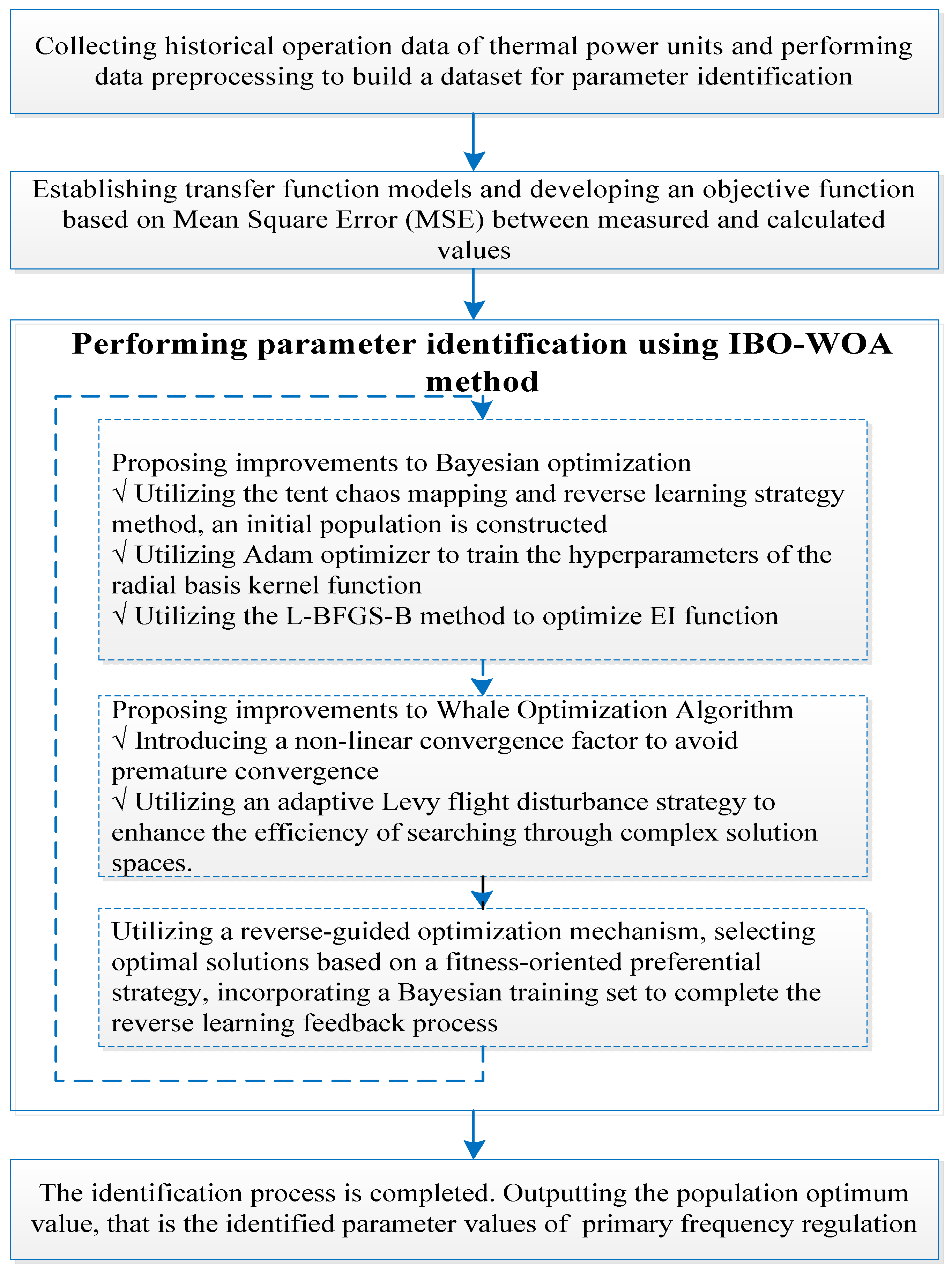
The overall idea of the IBO-WOA method was shown in Figure 1.
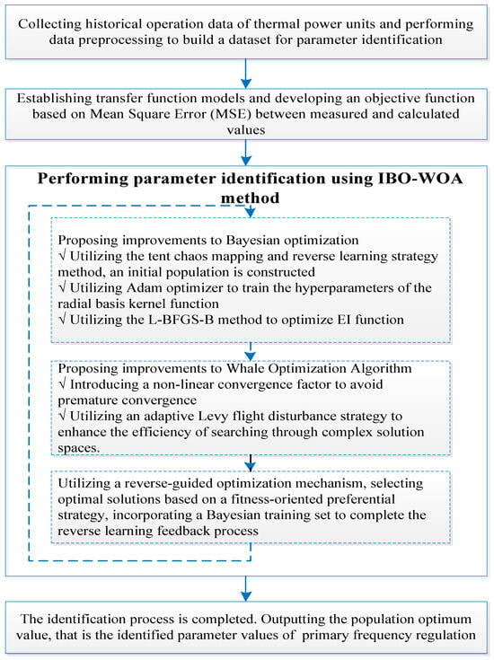
Figure 1.
The overall idea of the IBO-WOA method.
The specific steps were as follows:
- (1)
- Collecting historical operational data of multiple signals of a steam turbine. Performing data preprocessing, removing bad points from massive operating data, screening out operating data that can better represent different stable operating conditions, and constructing a parameter identification dataset.
- (2)
- Analyzing system characteristics for parameters to be identified, establishing transfer function models, and developing an objective function based on Mean Square Error (MSE) between measured and calculated values.
- (3)
- Using the IBO-WOA method for parameter identification of the objective function.
- (i)
- By using Tent chaotic mapping and the reverse learning strategy, an initial population with strong search potential was constructed, significantly enhancing the global search ability of the algorithm and avoiding premature convergence. By adopting a radial basis kernel hyperparameter training mechanism based on the Adam optimizer, the accuracy and optimization efficiency of the BO model were improved. By applying the L-BFGS-B method to optimize the EI function, candidate point selection achieved higher precision and speed. So, IBO was proposed to obtain the optimal candidate set with the smallest objective function value.
- (ii)
- By introducing a nonlinear convergence factor, the exploration and development capabilities of WOA were dynamically balanced to avoid premature convergence. By adopting the adaptive Levy flight disturbance strategy, breaking through local optimal barriers and improving the efficiency of complex solution space search. So IWOA was proposed to obtain locally optimized optimal solutions.
- (iii)
- By utilizing the reverse-guided optimization mechanism, a fitness-oriented optimization strategy was used to select optimal solutions, which were then imported into the Bayesian training set to further improve the overall exploration width and depth of the algorithm, completing the closed-loop process of reverse learning feedback.
- (4)
- After completing one identification optimization cycle, the algorithm evaluated whether the termination conditions have been met. If not, it repeated step (3); if yes, it output the population optimum value that was the identified PFR parameter values. The termination criterion was as follows: when the improvement of the global optimal solution over 20 consecutive iterations was less than a very small positive value ε (1 × 10⁻⁶), or when the preset maximum iterations number was reached, the algorithm stopped and output the results. Based on experience, we selected a relatively large integer as the maximum iterations number to ensure the algorithm has enough iteration space before reaching a stable state.
2.2. Implementation of the IBO-WOA Method
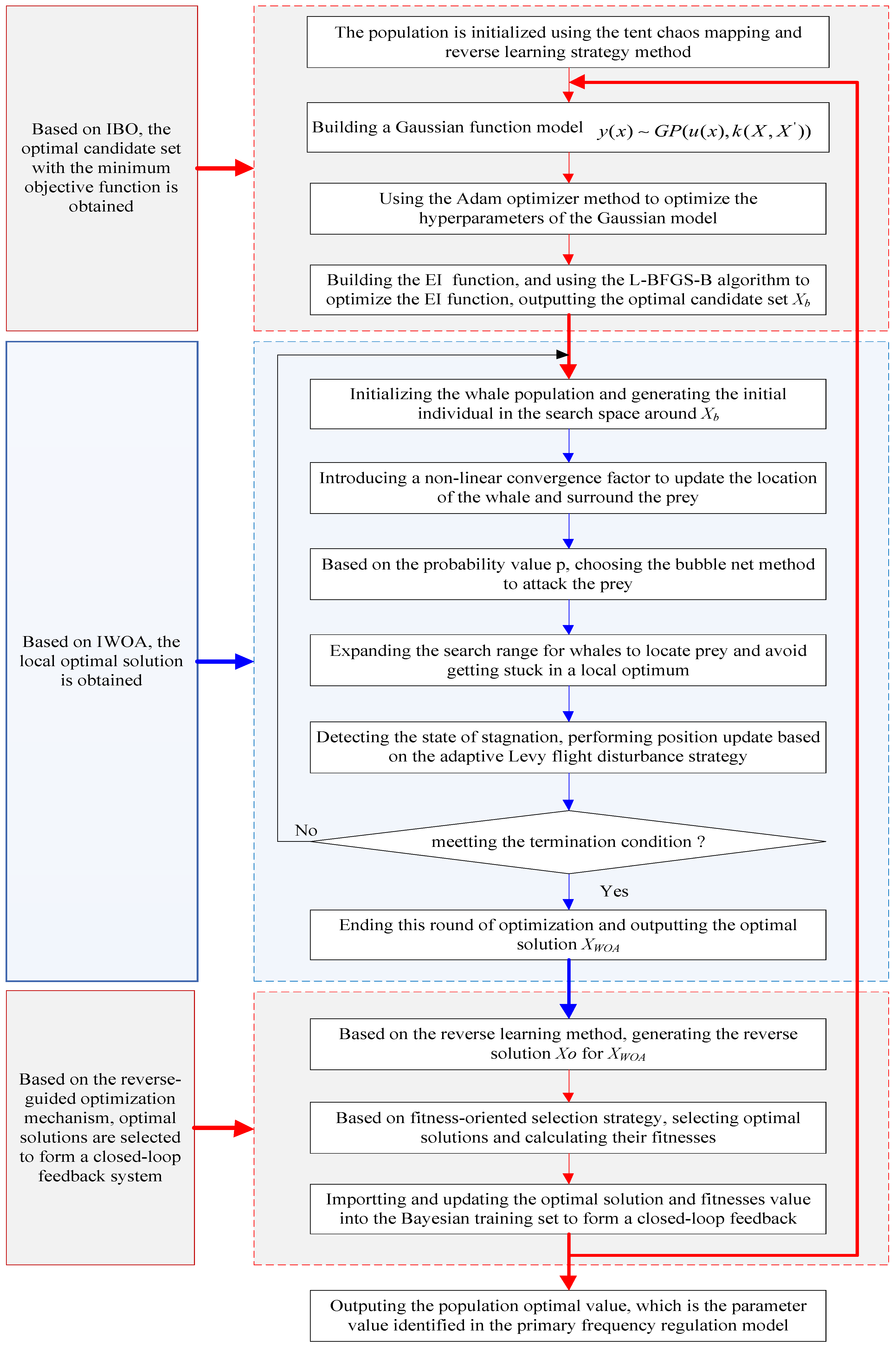
The process of the IBO-WOA method is shown in Figure 2.
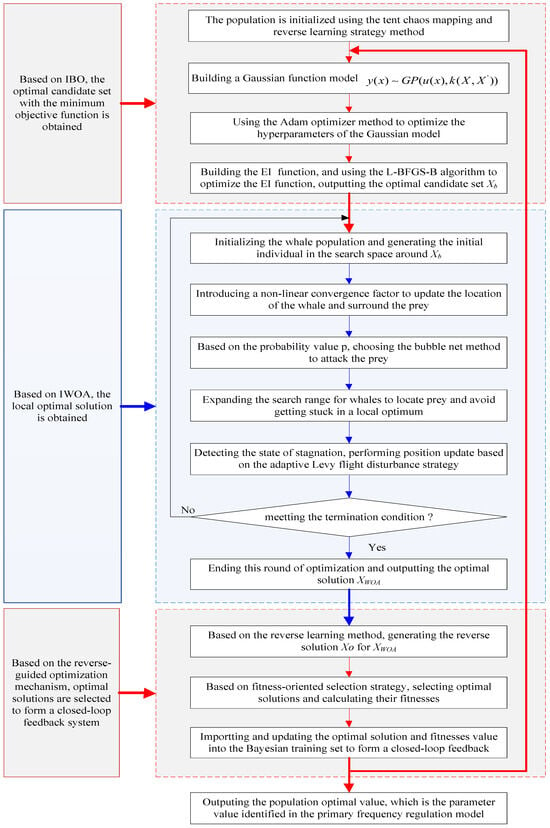
Figure 2.
Flow chart of the IBO-WOA method.
2.2.1. Implementation of the IBO Method
BO is a sequential sampling strategy based on the Gaussian process (GP), which is employed to solve black-box function optimization problems [18]. This paper improves BO by using Tent chaotic mapping and the reverse learning strategy to construct an initial population with strong search potential in population initialization. In terms of Gaussian model hyperparameter optimization, a radial basis kernel function hyperparameter training mechanism based on the Adam optimizer was adopted to achieve fast and robust optimal parameter search and improve optimization efficiency. Using L-BFGS-B to optimize the EI function and achieve global extremum exploration of the EI function at low computational cost, improved the accuracy and speed of candidate point selection. The specific steps of the proposed IBO method are as follows:
(1) Population initialization
The initial population in BO is typically generated randomly, which has the drawback of low global search efficiency. To overcome this limitation, this paper employs Tent chaotic mapping combined with the reverse learning strategy for population initialization. The principle is as follows: First, generate an initial population covering the entire range through Tent chaotic mapping (as shown in Equation (1)). Then, create a corresponding reverse population using the reverse learning strategy (as detailed in Equations (2) and (3)). After merging both populations, they are sorted by fitness value, with the top N best fitness values retained as the initial population NS. This method can effectively improve the quality of the initial solution and get closer to the global optimal region, so as to speed up the search for the global optimal.
The Tent chaotic mapping is used to generate the chaotic initial population , the expression is as follows:
where is the chaotic control parameter, ∈ [1.8, 2.0].
By adopting the reverse learning strategy, the reverse solution of each individual is generated to obtain the reverse solution of the chaotic initial population. The two together constitute the initial population X, and the expressions are as follows:
where lb and ub are the search boundaries of the parameters.
(2) Establishing the Gaussian model
GP is a parameter-free Bayesian model used to approximate an unknown objective function. For the unknown parameters , their objective functions are . The GP is used as the prior distribution of the objective function, which is expressed as follows:
where is the mean function, initialized to the mean of the training data; is the covariance function, determining the function form. The radial basis kernel function is selected as the core component of the covariance function, which is expressed as follows:
where l is the length scale, which measures the influence of input parameter changes on function output; is the signal variance, indicating the range of function output variation under zero mean; and is the noise variance.
(3) Gauss model hyperparameter optimization
To further enhance the search accuracy of BO, the hyperparameters of the Gaussian model are optimized by maximizing the marginal log-likelihood function. The model can best fit the observed distribution of the objective function, improving prediction accuracy and generalization ability. The expression is as follows:
where y is the observed value; K is the kernel matrix, which maximizes the observed distribution of the objective function to improve the prediction accuracy and generalization ability; I represents the independent and identically distributed characteristics of the observed noise; and C is the normalization constant of the probability distribution.
Directly optimizing the above objective function often faces multidimensional and non-convex numerical optimization problems [19,20]. To enhance computational efficiency and stability, we employ the Adam optimizer during the gradient descent phase of GP training. This method suppresses gradient oscillations and accelerates convergence by simultaneously tracking exponentially weighted moving averages of both first-order and second-order moments, with the specific implementation steps as follows:
(1) The Adam optimizer parameters are initialized, including the learning rate η, the exponential decay rate β1 for the first-order moment estimation, the exponential decay rate β2 for the second-order moment estimation, and the numerical stability correction ϵ. Typical values are η = 10−3, β1 = 0.9, β2 = 0.999, and ϵ = 10−8, with initial first-order moment vector m0 = 0 and second-order moment vector v0 = 0.
(2) Parameter optimization based on the Adam optimizer. Based on calculated loss values, the Adam optimizer employs a backpropagation algorithm to compute gradients for each parameter. The chain rule is used to determine the gradient ∇θ, L(θ) under current hyperparameters, where L(θ) = −ℓ(θ). To avoid direct matrix inversion, the Cholesky decomposition is applied in kernel matrix calculations to solve α = K − 1y.
(3) Rectification update and deviation correction. Updating and performing a deviation correction to obtain m^t and v^t, ensuring accurate estimation in the initial stage. The iterative update of the hyperparameters is as follows:
This process is performed in the hyperparameter training phase of each iteration of BO to ensure that the GP model always uses the latest and most optimal set of hyperparameters during the function evaluation.
According to the above update rules, the Adam optimizer uses gradient information to adjust the parameters, so that the model can be closer to the true value in the subsequent prediction, and then gradually reduce the loss value.
(4) Constructing the EI function
As parameters are continuously updated, posterior probabilities are obtained. To further optimize the objective function, BO utilizes the collection function to obtain the global optimum of f(x). During each iteration, the collection function balances high mean values with high volatility to select appropriate sample points for hyperparameter selection. The EI explicitly measures how much the error of the next parameter set can be improved compared to the historical optimal, expressed as follows:
where is the best fitness of historical observation summary; is exploration-use of trade-off factors, general values (0.01,0.1); , represents the improvement rate and improvement density, respectively, which are calculated by table checking; is the predicted standard deviation, which represents the uncertainty of the model, it is usually taken as 0.005; and Z is a standardized measure of relative improvement, and its expression is as follows:
(5) Optimizing the EI function with the L-BFGS-B method
The generated candidate points cover the parameter space by evenly distributing initial candidates across the range [xmin, xmax]. Using the EI function shown in Equation (8), we calculate EI values for all candidates. The historical optimal fitness value is determined by the minimum objective function value from the current training set. The top 5 high EI points are selected as parallel initial points for the L-BFGS-B method. Independent optimization threads are initiated for each point with maximum function evaluations and strict boundary constraints. After each thread optimization completion, the results are merged to select the parameter combination with the minimum objective function value as the optimal candidate set Xb, while simultaneously outputting its fitness value.
2.2.2. Implementation of the IWOA Method
WOA is a meta-heuristic optimization algorithm that simulates the hunting behavior of humpback whales to find optimal solutions. Assuming the whale population size is N and the dimension of the problem-solving space is D, the optimal position for the i whale in the D-dimensional space would be , i = 1,2,3,…,N. Then the optimal position of the whale corresponds to the optimal solution of the problem [21]. WOA has a simple principle and few parameter settings, but it lacks population diversity, has poor global search ability, and is prone to falling into local optima. To address these shortcomings, this paper introduces a nonlinear convergence factor and the adaptive Levy flight disturbance strategy to enhance WOA. The specific steps are as follows:
- (1)
- Initializing the whale population
Centered on the optimal candidate set Xb output by IBO, initial individuals are generated in search space .
- (2)
- Surrounding prey
During the hunt, the whale first observes and identifies the location of the prey, then surrounds it. The distance between an individual and the optimal solution (the prey) is calculated by the following equation:
where t is the current iteration number; is the current whale position vector; is the current optimal solution, that is, the position of the prey; and C is the swing factor, calculated as follows:
where r2 is a random number between [0, 1].
The whale position update formula is as follows:
where A is the matrix coefficient expression, and the calculation expression is as follows:
where r1 is a random number between [0, 1]. a is the convergence factor. Typically, a decreases linearly from 2 to 0 as the iteration count increases. However, this linear reduction approach often leads to issues such as insufficient exploration, premature termination of exploration, and inadequate development in later stages. To address these problems, this paper introduces a nonlinear convergence factor expressed as follows:
where amax is a constant with a value of 2. k is a constant that controls the descent rate of the convergence factor, the larger its value, the faster the rate of decline in later iterations, and k > 0. P is a constant that regulates the plateau length during exploration, meaning the first 100p% of iterations maintain a larger value, p∈(0, 1)). is the maximum iteration number.
The nonlinear convergence factor enables precise control over the platform length during the initial search phase. By maintaining a relatively stable value of α throughout this stage, it allows for larger step sizes to expand the search scope, effectively addressing issues of insufficient exploration or premature termination. After transitioning from the exploration phase to the development phase, the value of a rapidly decreases to nearly 0, accelerating the convergence speed in the later stage and achieving high-precision convergence.
- (3)
- Bubblenet attacks preyWhales attack their prey in two ways: by contracting and surrounding prey, or by spiraling out and blowing bubbles.
- (i)
- Contracting and surrounding preyThe whale position is obtained by Equation (12), and the position is achieved by nonlinearly decreasing the convergence factor a from 2 to 0, where A is a random number in [−1, 1].
- (ii)
- Spiraling out and blowing bubblesThe first step is to calculate the distance between each individual whale and the current best position, and then simulate whales using a spiral upward method for calculation during hunting. The expressions are as follows:where D represents the distance between the ith whale and the current optimal position (optimal solution); b is a constant coefficient used to limit the spiral form; l is a random number between [−1, 1], where l = −1 indicates the whale is closest to the prey, and l = 1 indicates the whale is farthest from the prey.
When the whale uses the spiral upward form to surround the prey, it also needs to shrink the circle surrounding, and choose the same probability p to shrink the surrounding and spiral update the optimal solution. The expression is as follows:
- (4)
- Hunting prey
To expand the whale search range and avoid getting trapped in local optima, this phase of the algorithm no longer updates its position based on the currently optimal prey but instead updates according to randomly selected whales [22]. Specifically, to enhance global search capability and prevent local optimization, when the random probability p ≥ 0.5, if |A| ≥ 1, the distance D is randomly updated. The mathematical model simulating whale searching can guide other whales by randomly selecting an individual whale . The specific expression is as follows:
where is the current position vector of the randomly selected whale.
- (5)
- Position update based on the adaptive Levy flight disturbance strategy
After each iteration, the system monitors for stagnation. If the optimal solution remains unchanged through multiple consecutive iterations, the adaptive Levy flight disturbance mechanism is activated. The Levy flight is a walking pattern combining short-distance searches with occasional long-range movements, it can explain many random phenomena in nature, such as Brownian motion, random walks, etc. When applied to WOA, this mechanism enhances population diversity, expands search coverage, and improves local optimum escape capabilities. The position update formula is as follows:
where α is the step size coefficient that controls the disturbance intensity, typically set to 0.1; β denotes the heavy-tailed distribution degree, with 1.5 balancing exploration; μ and v are the Gaussian random vector and the unit Gaussian random vector, respectively, controlling the direction and magnitude of the disturbance. Enforcement of boundary constraints .
- (6)
- After the iteration ends, the optimal solution XWOA of whale optimization is output.
2.2.3. Reverse-Guided Optimization Mechanism
The reverse-guided optimization mechanism is used to select the optimal solution based on the fitness-oriented optimization strategy, and the feedback is returned to the Bayesian training set to complete the closed-loop process of reverse learning feedback. The specific steps are as follows:
(1) For the optimal solution XWOA of IWOA, its reverse solution Xo is generated according to Equation (2);
(2) The fitness values and of the optimal solution XWOA and the reverse solution Xo are calculated, respectively;
(3) Selecting based on the fitness-oriented optimization strategy:
If , Then the best result is obtained by reverse solution, ; if not, . And calculate the fitness value .
(4) Importing the preferred solution into the Bayesian training set . The initial training set is updated as the input of the next round of BO, forming a closed-loop process of “Bayesian global exploration → whale local optimization → reverse learning feedback”.
The synergistic effect of IBO and WOA is grounded in the complementary optimization paradigms of both algorithms and the profound theoretical reinforcement of global exploration capabilities by the reverse-guided feedback mechanism. IBO constructs a global probabilistic landscape through Gaussian processes, with its gradient-based hyperparameter optimization mechanism excelling in high-precision local exploitation. The improved WOA, through adaptive Levy flight perturbations regulated by a nonlinear convergence factor, focuses on efficient global exploration and local hunting. The core theoretical advantage of the reverse-guided feedback mechanism lies in overcoming the inherent limitations of sequential uncoupled optimization strategies. Sequential strategies are inherently unidirectional in the information transfer, where the output of the preceding algorithm serves as fixed input for the subsequent one. Potential suboptimal solutions or insufficiently explored regions from the preceding stage are difficult for the subsequent algorithm to effectively correct, constraining the breadth and depth of global search. The reverse-guided mechanism in this work dynamically feeds the optimization results of WOA and their reverse solutions back into the IBO training set based on fitness-oriented selection. This process injects and calibrates the IBO’s global probabilistic model in real-time with critical solution space information discovered during the WOA exploration, particularly potential high-quality regions distant from the initial population revealed through Levy perturbations. This closed-loop feedback significantly enhances the representational accuracy of the IBO surrogate model regarding the structure of complex multimodal solution spaces, thereby systematically strengthening the algorithm’s proactive exploration guidance capability towards unknown high-quality regions. This fundamentally enhances the robustness against local optima entrapment and the overall global optimization performance.
2.3. Case Analysis Setup
In order to verify the feasibility and superiority of IBO-WOA, simulations were conducted on nine standard test functions and a 330 MW steam turbine, and compared with four algorithms: PSO, WOA, BO, and PSO-GWO.
2.3.1. Standard Test Functions Case
Nine standard test functions are categorized into three types: unimodal functions, non-fixed-dimensional multi-modal functions, and fixed-dimensional multi-modal functions, as detailed in Table 1. Specifically, f1~f3 are unimodal functions designed to test the global exploration capability; f4~f6 are non-fixed-dimensional multi-modal functions; and f7~f9 are fixed-dimensional multi-modal functions. These multi-modal functions are employed to evaluate the global exploration capability and escape local optima capability.

Table 1.
Standard test functions.
This study compares IBO-WOA with PSO, WOA, BO, and PSO-GWO through 30 independent runs, each with a maximum iteration count of 200. Performance metrics include: the average value, standard deviation value, and fitness function convergence curve comparison of different test functions.
2.3.2. 330 MW Steam Turbine Case
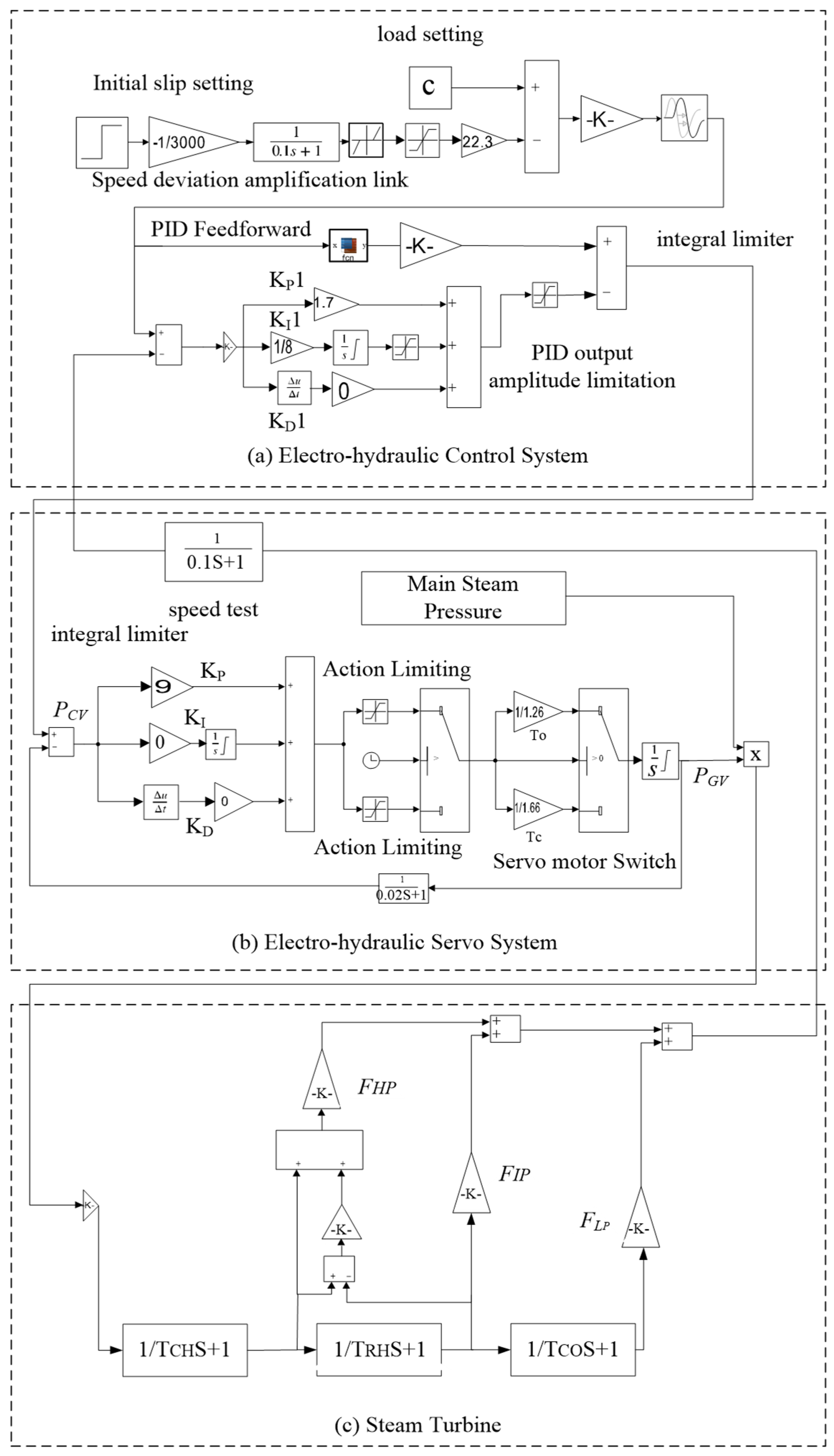
Taking a 330 MW steam turbine as the research object, the unit adopts a regulating valve pre-throttling method for PFR, which performance is affected by the models and parameters of the electro-hydraulic control system, electro-hydraulic servo system, and steam turbine. The established PFR model is shown in Figure 3. Some parameters in the model need to be identified and confirmed through unit operation data, and the accuracy of their identification results affects the accuracy of the PFR simulation analysis.
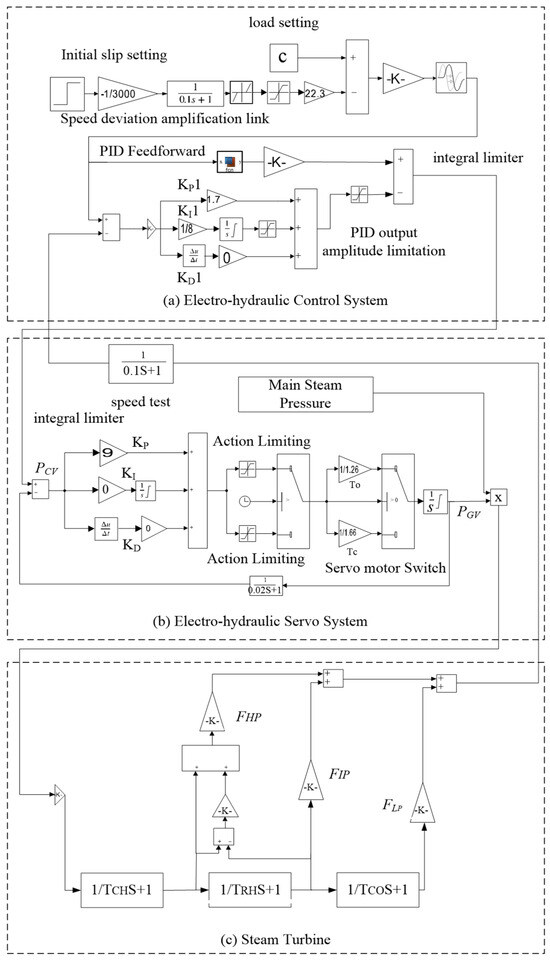
Figure 3.
PFR model of 330 MW steam turbine.
It should be noted that IBO-WOA is only validated on a 330 MW steam turbine, as there are specific differences in the speed automatic control system of a steam turbine generators of different capacity levels and technological generations. If IBO-WOA is to be extended to full capacity units, appropriate adjustments need to be made based on the characteristics of the units. The concepts of “dead band of primary frequency regulation” and “intensive (normalized) frequency regulation” in frequency control necessitate enhanced frequency identification accuracy during parameter identification for PFR. The reason lies in: improved accuracy ensures that generating units can respond timely, accurately, and reliably when frequency crosses the “dead band” boundary, preventing oscillatory behavior around the threshold and avoiding false trips or failure to operate; It enables a near-synchronous response from steam turbine units, allowing numerous conventional units to form a stable and predictable power response. This seamlessly integrates with the “power spikes” provided by gas turbine units and power storage systems, collectively establishing a continuous and stable frequency defense system operating from seconds to minutes. Meanwhile, improving power system frequency control quality also carries certain negative implications. It may lead to an increase in operational and maintenance costs and shorten maintenance intervals due to more frequent actuation of control valves. Therefore, careful consideration must be given to the setting of the “dead band of primary frequency regulation.”
For a 330 MW steam turbine, a simulation verification of the PID parameter identification of the electro-hydraulic servo system was first carried out. Then, experimental verifications were conducted on the identification of steam turbine time constants, which were applied to the modeling and analysis of the PFR simulation.
(1) PID parameter identification of the electro-hydraulic servo system
Taking the PID parameter identification of the electro-hydraulic servo system as an example, we utilize known parameters to verify the feasibility and superiority of IBO-WOA. The model of this electro-hydraulic servo system is shown in Figure 3b. In the figure, , , KD are the proportional coefficient, integral coefficient, and derivative coefficient of the PID controller; PGV is the opening value position; PCV is the total valve position command of the unit; TR is the time constant of the Linear Variable Differential Transmitter (LVDT); , are the opening and closing time constants of the hydraulic servo-motor.
The PID parameters are set as = 9, = 0, KD = 0. According to the static test of the unit valve, the calculated is 1.26 s, is 1.66 s, and TR is 0.02 s.
The parameter identification is carried out by using step signal. The initial parameters of IBO-WOA are set as follows: population number = 40. Maximum iteration number of Bayesian = 10. Maximum iteration number of WOA . The population dimension dim = 2. KP is limited to [0, 30], and KI is limited to [0, 20].
To verify the robustness of IBO-WOA, an Out-Of-Distribution (OOD) Test based on noise injection was conducted for the electro-hydraulic servo system. The OOD Test can be used to evaluate the model’s generalization capability, robustness, and resilience to unknown scenarios, which is crucial for assessing the model’s practicality in real industrial settings. The dataset construction method was as follows: Based on the measured experimental data, Gaussian white noise was systematically added to each input parameter of experimental data to simulate data distribution shifts encountered in practical applications, thereby constructing the OOD Test dataset. To correlate the noise intensity with the original data scale, the amplitude of the white noise was based on the standard deviation of each input parameter. The white noise ratio was set to increase from 1% to 10% in increments of 1%, and followed a Gaussian distribution. The dataset after adding noise can be represented as follows:
where was the original dataset; was white noise, and its expression was follows:
(2) Steam turbine time constant identification
Steam turbine model is illustrated in Figure 3c, where FHP, FIP, and FLP represent the power coefficients of high-pressure, medium-pressure, and low-pressure cylinders, respectively, with set values of 0.29, 0.37, and 0.34. K is the power overshoot coefficient of the high-pressure cylinder, set to 1.1. TCH is the steam volumetric time constant of the high-pressure cylinder. TRH is the intermediate reheat volumetric time constant. TCO is the steam time constant of the low-pressure connecting tube. TCH, TRH, and TCO are the three parameters under identification.
The initial parameters of IBO-WOA are set as follows: population number = 40. Maximum iteration number of Bayesian = 10. Maximum iteration number of WOA . The population dimension dim = 2, and the exploration boundary is [0, 10].
In order to verify the generalization ability of IBO-WOA, parameter identification analysis was conducted for two different experimental conditions, and the model training data was obtained from on-site test data of the experimental conditions.
Experimental condition 1:
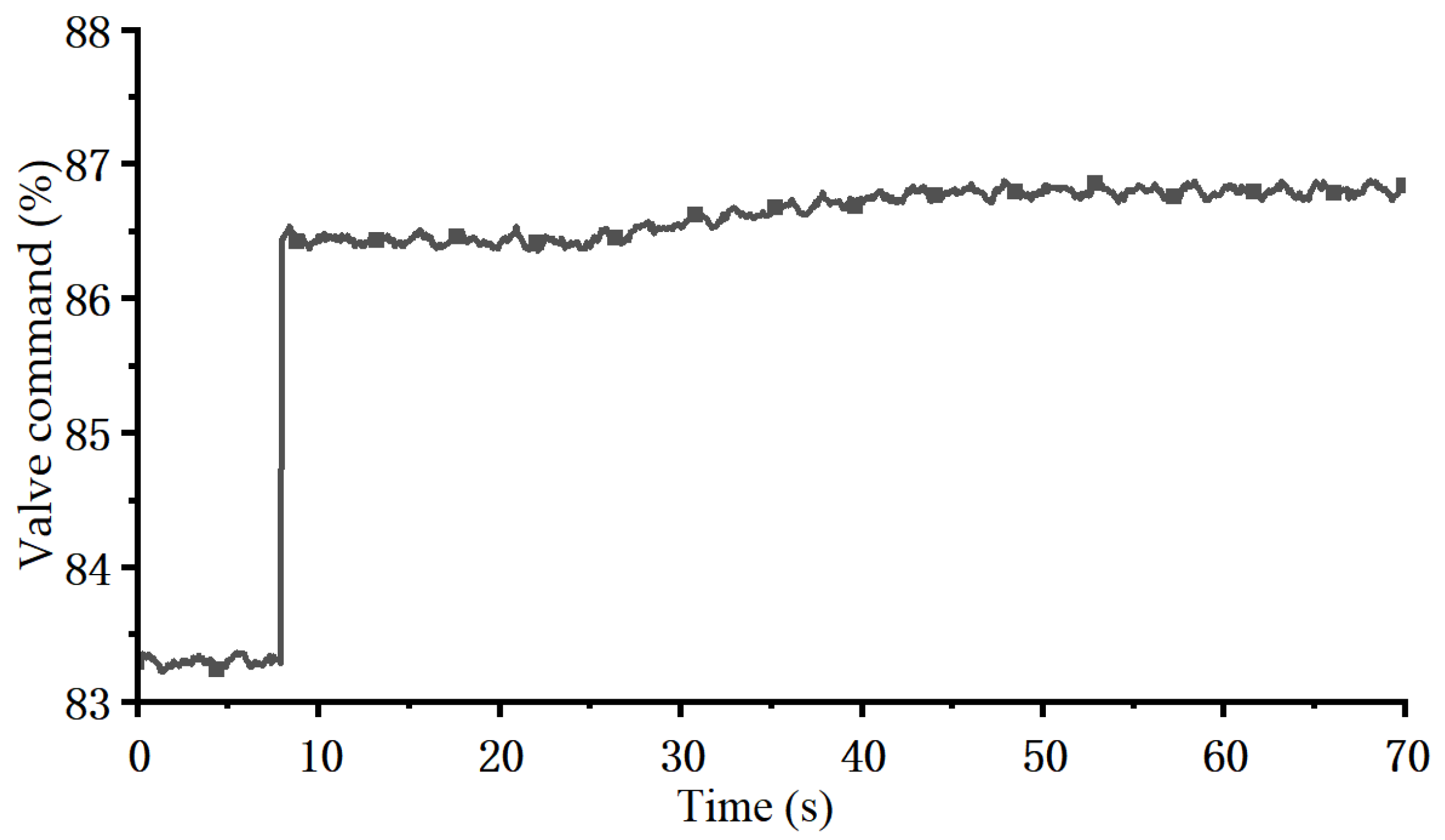
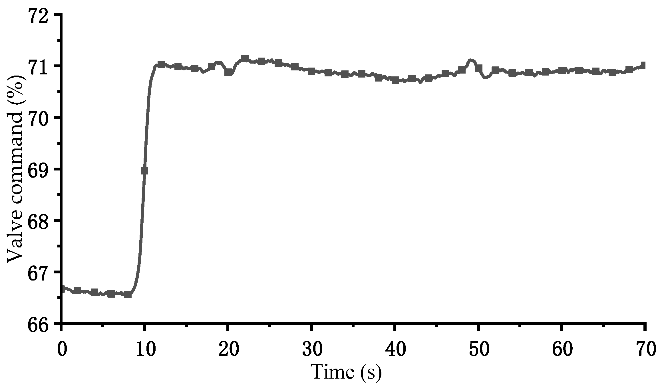
Based on actual PFR experimental data from this unit, parameter identification is conducted using a valve-controlled step disturbance test. The experimental condition 1 was as follows: before the experiment, the stable power of the unit was 275 MW. After about 8 s, the total valve position command increased by 3.2%, and the power increased by 10 MW. The measured change curve of the total valve position command of the unit was shown in Figure 4.
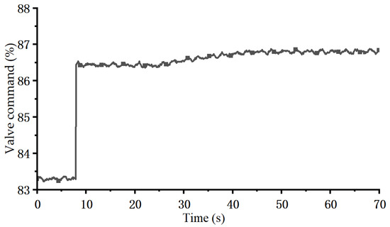
Figure 4.
Change curve of total valve position command under experimental condition 1.
Experimental condition 2:
The experimental condition 2 was as follows: before the experiment, the stable power of the unit was 174 MW. After about 8 s, the total valve position command increased by 4.4%, and the power increased by 8.8 MW. The measured change curve of the total valve position command of the unit was shown in Figure 5.

Figure 5.
Change curve of total valve position command under experimental condition 2.
2.3.3. Evaluation Metrics
To objectively and quantitatively evaluate the model performance proposed in this paper, five performance metrics are used, including Mean Squared Error (MSE), Root Mean Squared Error (RMSE), Mean Absolute Error (MAE), Mean Absolute Percentage Error (MAPE), and the determination coefficient (R2). By using five performance metrics to evaluate the identification results, the identification accuracy and reliability of the model can be comprehensively measured from different perspectives.
The equations for these performance metrics are as follows:
where is the number of samples in the dataset; is the actual value of the i-th sample in the dataset; and is the identification value of the i-th sample in the dataset.
MSE, RMSE, and MAE are used to measure the deviation degree between the identification value and the actual value. The smaller the value, the smaller the identification error and the higher the accuracy. MAPE represents the identification error as a percentage of the actual value, which can more intuitively reflect the relative error size of the identification result. The R2 reflects the fitness degree of the model, and the closer the R2 is to 1, the closer the identification result is to the actual value.
2.3.4. Experimental Platform
All experiments were conducted on a computer equipped with a 13th Gen Intel (R) Core (TM) i5-13500H (2.60 GHz) CPU and NVIDIA GeForce RTX 4050 Laptop 6 GB GPU, using Python 3.8 code developed on the PyCharm 2024.1.1 platform. Data processing and experiments were conducted on a Windows platform.
3. Results and Discussion
3.1. Standard Test Function Case
The test results of the five algorithms are presented in Table 2.

Table 2.
Analysis results of the five algorithms.
As shown in the table, for all test functions, IBO-WOA outperforms PSO, WOA, BO, and PSO-GWO in terms of optimal values, average values, and standard deviation values. This indicates that IBO-WOA has superior global search capability, regional optimization capability, and local optimal region escape capability. Its optimization results have higher accuracy, stronger stability, and robustness.
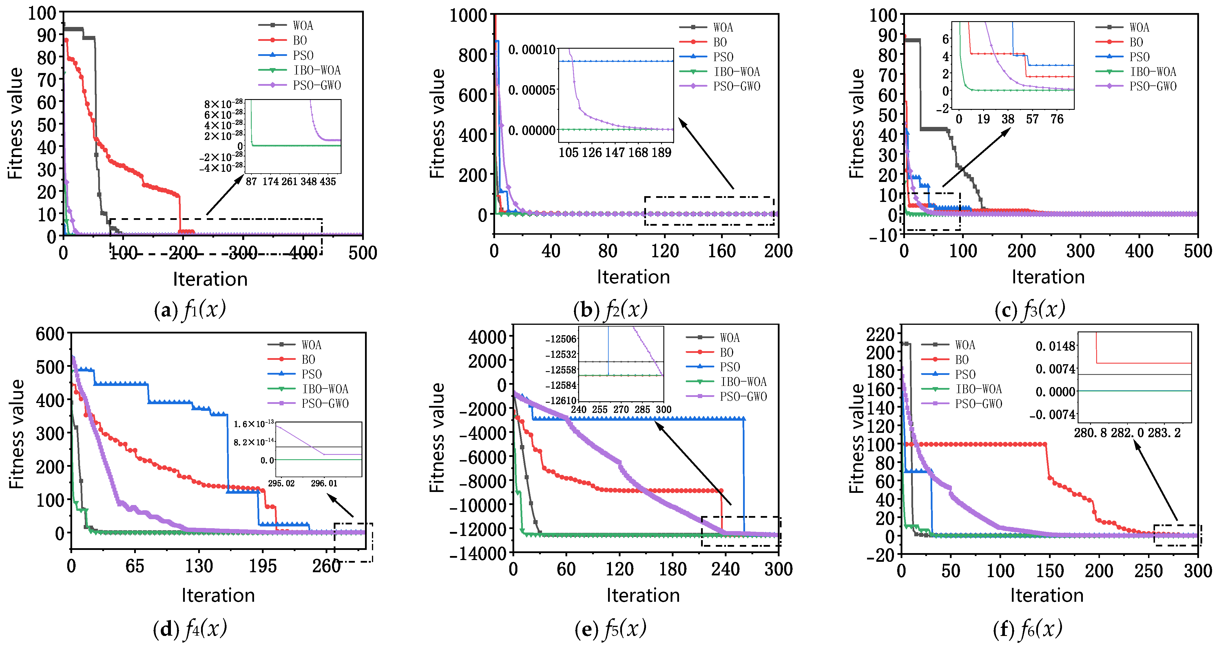
In order to compare the optimization performance of IBO-WOA with other algorithms more intuitively, Figure 6 shows the convergence curve of all five algorithms in the search for the optimal value of all standard test functions with increasing iterations.
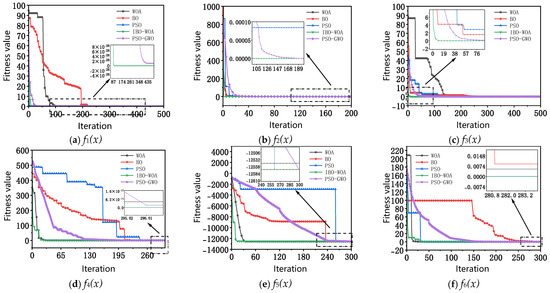

Figure 6.
Convergence curves of standard test functions.
Taking Figure 6a as an example, the optimization process curve of IBO-WOA is similar to that of a straight line approaching the optimal value, indicating that it has good global search ability and avoids getting stuck in local optima. After 11 iterations, the curve of IBO-WOA reaches the initial optimal value 8.21 × 10⁻²², which is very close to the theoretical optimal value 0. As shown in Table 2, its final optimized optimal value is 1.47 × 10⁻³¹. After 22 iterations, the curve of PSO reached the initial optimal value of 1.13 × 10⁻⁶, and after multiple iterations, the final optimized optimal value is obtained as 1.25 × 10⁻¹⁰. After 98 iterations, the curve of WOA reached the initial optimal value of 3.43 × 10⁻⁵, and after multiple iterations, the final optimized optimal value is obtained as 3.78 × 10⁻¹¹. After 219 iterations, the curve of BO reached the initial optimal value of 5.11 × 10⁻⁸, and after multiple iterations, the final optimized optimal value is obtained as 6.06 × 10⁻¹⁵. After 352 iterations, the curve of PSO-GWO reached the initial optimal value of 4.58 × 10⁻¹, and after 418 multiple iterations, the final optimized optimal value is obtained as 1.01 × 10⁻²⁸.
Similar conclusions can also be drawn from other figures. It can be seen that regardless of whether it is a uni-modal or multi-modal function, compared to the other four algorithms, IBO-WOA has the fastest convergence speed and the highest convergence accuracy, indicating its excellent global search performance and excellent ability to jump out of local optima. Moreover, the initial optimal value of IBO-WOA is significantly better than the other four algorithms, which fully proves that Tent chaos initialization can make the initial population distribution more uniform, and has good initial optimization accuracy at the beginning of the iterations.
The test time results of five algorithms are shown in Table 3. As shown in the table, for all test functions, although IBO-WOA performs well in parameter identification accuracy and convergence degree, its running efficiency is relatively low, and the running time consumed is higher than that of the other four algorithms. This is mainly due to the fusion of IBO and IWOA in the IBO-WOA method, and the introduction of improvement strategies to enhance accuracy and escape from local optima within IBO and IWOA. At the same time, a three-layer collaborative framework of “Bayesian global guidance-whale local optimization-reverse learning feedback” is constructed, which is executed 10 times per iteration cycle, significantly increasing computational complexity. The results indicate that while IBO-WOA improves optimization performance, it also increases the computation time accordingly. In practical applications, a balance between accuracy and efficiency needs to be comprehensively considered.

Table 3.
The running time of five algorithms(s).
3.2. PID Parameter Identification Cases of Electro-Hydraulic Servo System
The electro-hydraulic servo system in Figure 3b is a typical single input single output model, ignoring the amplitude limiting step. Its transfer function is expressed as follows:
where is the calculated valve opening through the transfer function.
Substituting = 1.26, = 1.66 into the above equation, then it is transformed into the following:
3.2.1. PID Parameter Identification
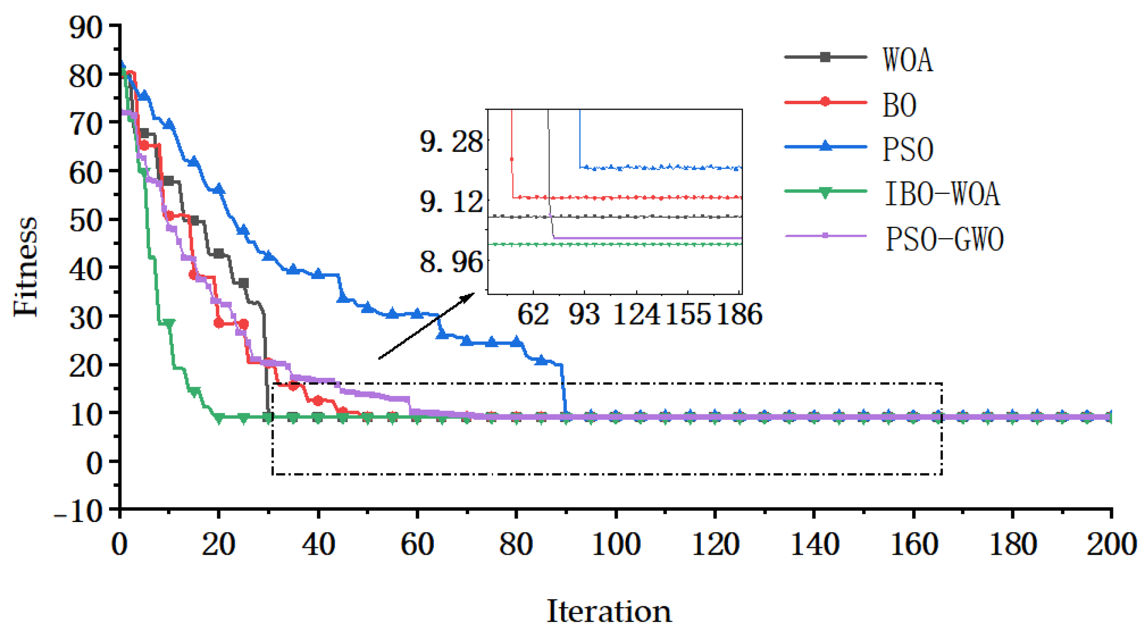
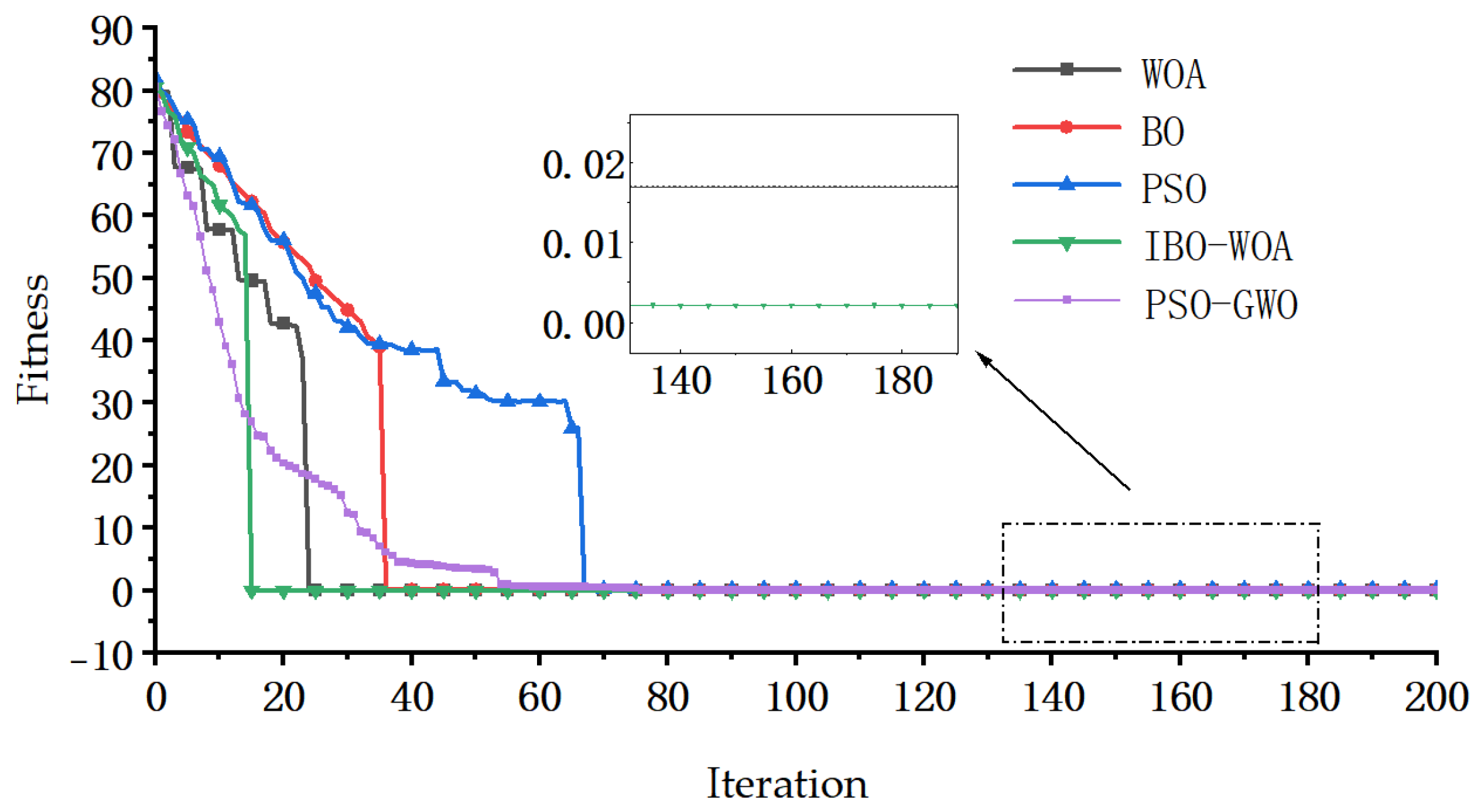
The five algorithms IBO-WOA, PSO, WOA, BO, and PSO-GWO are used for parameter identification, respectively. The optimal value identification curve of is shown in Figure 7. The optimal value identification curve of is shown in Figure 8, and the parameter identification results of the five algorithms are shown in Table 4.
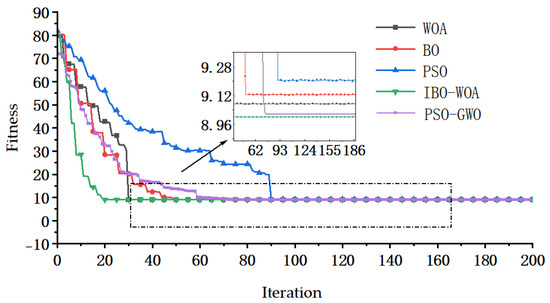
Figure 7.
The optimal value identification curve of KP.
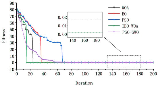
Figure 8.
The optimal value identification curve of KI.

Table 4.
Parameter identification results of five algorithms.
It can be seen from Table 4 and Figure 7 that in the parameter identification process of , the curve of IBO-WOA stabilizes after 19 iterations, achieving an identification result of 9.002 with MSE of 0.022. The curve of PSO stabilizes after 90 iterations, achieving an identification result of 9.202 with MSE of 2.244. The curve of WOA stabilizes after 31 iterations, achieving an identification result of 9.075 with MSE of 0.833. The curve of BO stabilizes after 51 iterations, achieving an identification result of 9.128 with MSE of 1.422. The curve of PSO-GWO stabilizes after 80 iterations, achieving an identification result of 9.017 with MSE of 0.289. It can be seen that compared to the other four algorithms, IBO-WOA has the fewest number of iterations towards stability, the smallest relative error in the final identification result, and the highest accuracy. The variation pattern of the optimal parameter identification curve in Figure 8 is also similar to that in Figure 7. This simulation case validates the feasibility and superiority of IBO-WOA.
3.2.2. Analysis of Influencing Factors
There are many factors affecting IBO-WOA performance, primarily including the population size N, the nonlinear convergence factors k and p. These parameters determine the exploration–exploitation balance, search diversity, and convergence speed of the algorithm. Improper settings may lead to premature convergence, local optima entrapment, or wasted time; moreover, the randomness of the algorithm causes significant fluctuations in individual results, making it necessary to conduct a systematic analysis of influencing factors. The following analysis is conducted using the KI identification of the electro-hydraulic servo system as an example.
(1) Population size N
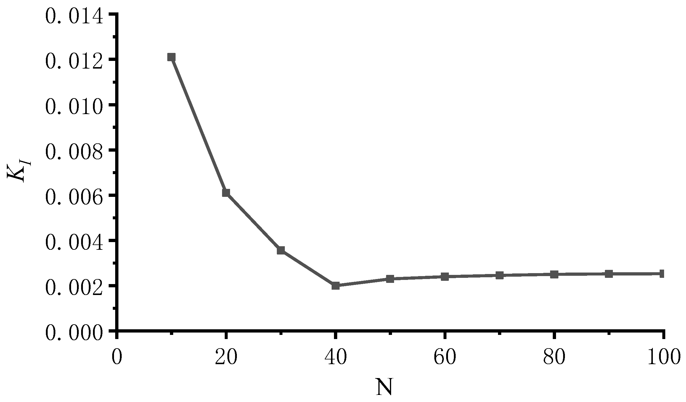
Figure 9 illustrates the variation of KI identified by the IBO-WOA as the population size N increases from 10 to 100. As shown in the figure, the IBO-WOA is relatively sensitive to changes in population size N. When N increases from 10 to 40, the identified KI rapidly decreases from 0.012 to 0.002, a reduction of approximately 83%. As N continues to increase from 40 to 100, the identified KI gradually rises from 0.0020 to 0.0024, while the runtime increases approximately linearly with N. Considering both identification accuracy and efficiency, the optimal population size N is determined to be 40.

Figure 9.
KI changes with N.
(2) Nonlinear Convergence Factors k and p
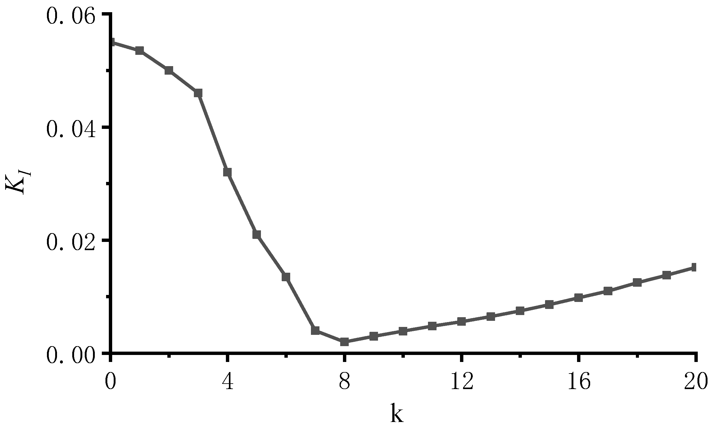
The nonlinear convergence factors k and p together determine the decay curve of the control parameter and the switching rhythm between exploration and exploitation. k primarily regulates the curvature of the decay, while p deepens or slows the nonlinear amplitude of the decay. If k or p is too small, it will prolong early exploration and delay effective exploitation, resulting in slow performance improvement of IBO-WOA and limited final accuracy. Conversely, if k or p is too large, the parameter shrinks too quickly, causing the algorithm to enter the exploitation phase too early and easily fall into local optima, which in turn increases K. By setting the population size N = 40 and gradually increasing K from 0 to 20, the variation curve of KI identification results with K is obtained, as shown in Figure 10. From the figure, it can be seen that as K increases, KI first gradually decreases and then slowly increases. When K = 8, KI reaches the lowest value of 0.0021; therefore, the optimal value of K is determined to be 8.
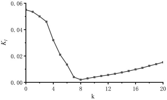
Figure 10.
KI changes with k.
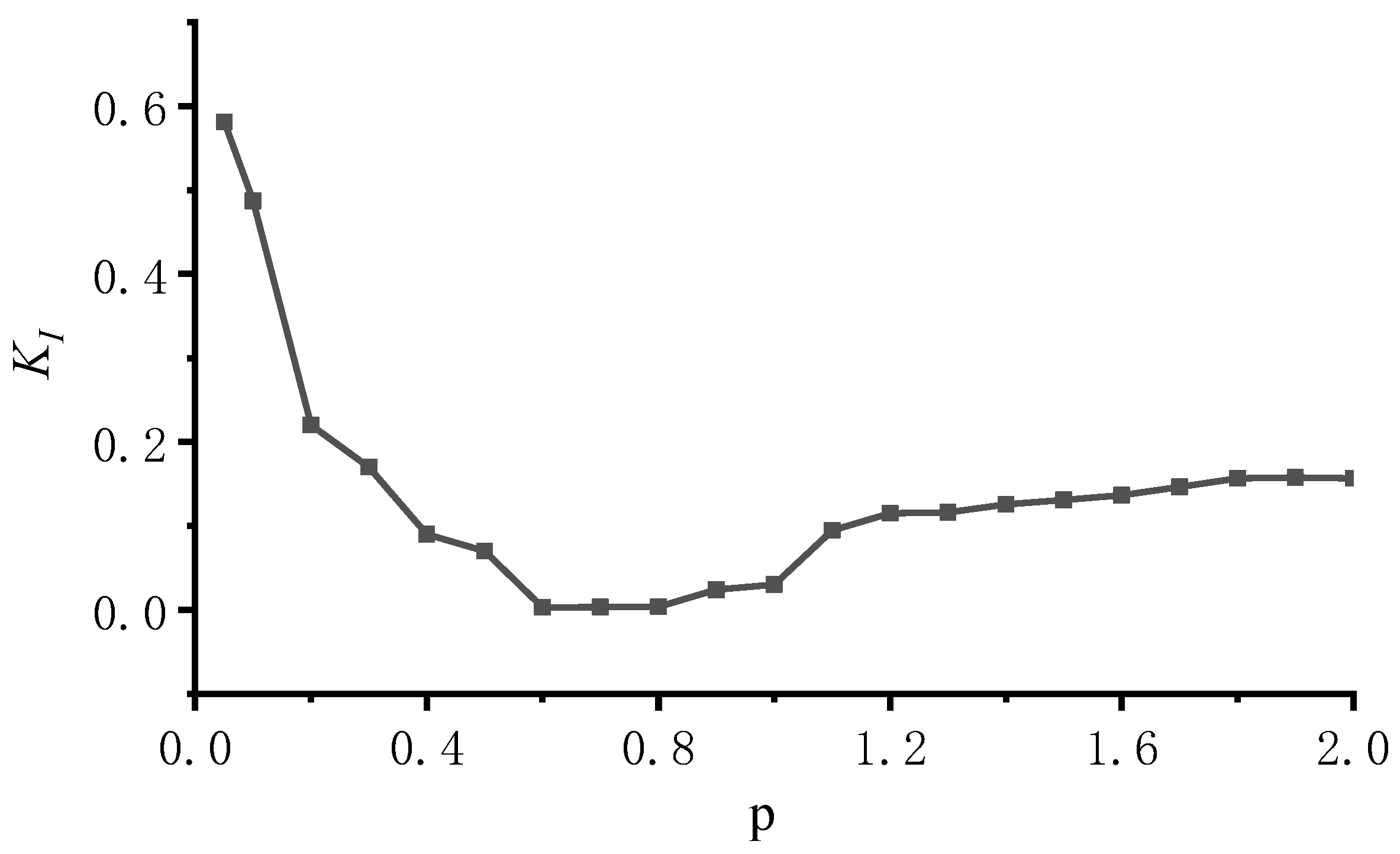
Set the population size N = 40, k = 8, and let P gradually increase from 0 to 2.0. The variation curve of the KI recognition results with p is obtained, as shown in Figure 11. From the figure, it can be seen that as p increases, KI first gradually decreases and then slowly increases. When p = 0.8, KI reaches its minimum value of 0.0016, so the optimal value of p is determined to be 0.8.

Figure 11.
KI changes with p.
3.2.3. OOD Test Based on Noise Injection
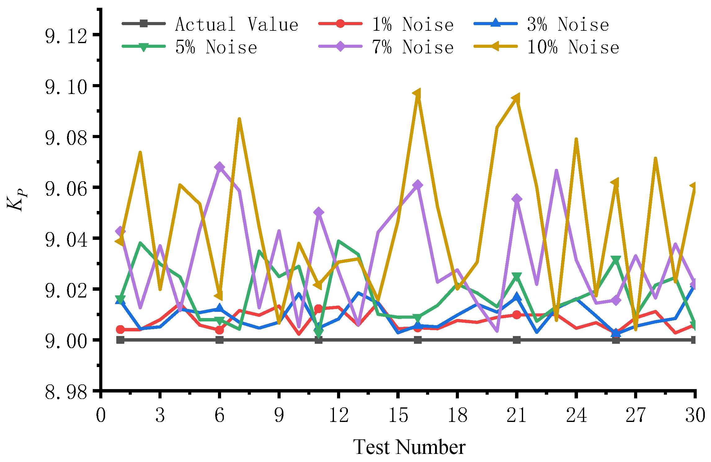
Based on the testing dataset with added noise, OOD Test is conducted on IBO-WOA. Taking the KP identification of the electro-hydraulic servo system as an example, 30 tests were conducted for each noise ratio. The test results for various metrics are shown in Table 5. Taking the scenarios with 1%, 5%, and 10% added noise as examples, the resulting identification curves are depicted in Figure 12.

Table 5.
OOD Test results for various metrics of IBO-WOA.
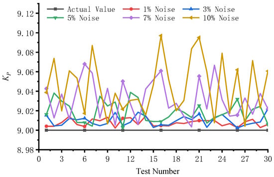
Figure 12.
KP identification curves with different white noise.
As shown in Table 5, with increasing white noise, MSE, RMSE, MAE, and MAPE all increase to varying degrees, while R2 continues to decrease. This indicates a decline in the robustness of IBO-WOA. Similar observations can be made in Figure 12: as white noise increases, the identification curve deviates further from the actual value, indicating a deterioration in identification accuracy. Taking the R2 metric as an example, at a 1% white noise level, the model’s R2 remains as high as 0.9991. This indicates that under minor distribution shifts, the model’s performance degradation is negligible. Even when the noise proportion increases to 5%, the R2 value remains robustly at 0.9863, while the MSE also remains relatively small. This demonstrates that IBO-WOA exhibits strong robustness against mild to moderate data perturbations and possesses reliable performance and practical potential when handling noisy and fluctuating data commonly encountered in real industrial processes.
3.3. Steam Turbine Time Constant Identification Cases
Taking TCH identification as an example, its transfer function is as follows:
where Ptjj is governing stage pressure. PCV is the total valve position command. K is the steady-state gain coefficient, which is calculated by the total valve position command and the governing stage pressure when the unit runs in a disturbance-free state.
Taking the total valve position command as the input and the governing stage pressure as the output, TCH is identified by the IBO-WOA, PSO, WOA, BO, and PSO-GWO algorithms, respectively, based on the above transfer function. To verify the adaptability of the algorithms, time constant parameter identification is conducted for two different experimental conditions.
3.3.1. Experimental Condition 1
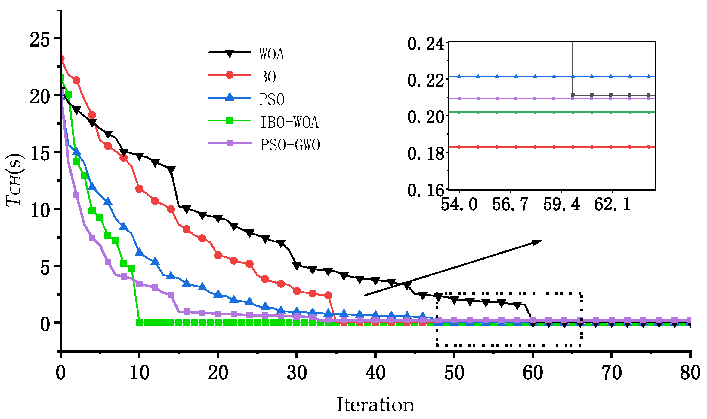
The TCH identification curve during the identification process is shown in Figure 13. It can be seen that the identification results of the five algorithms are relatively close. Taking IBO-WOA as the standard, after 12 iterations, it tends to be stable, and the final identification result of TCH is 0.202 s.
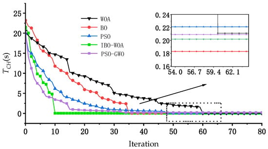
Figure 13.
TCH identification curves of five methods.
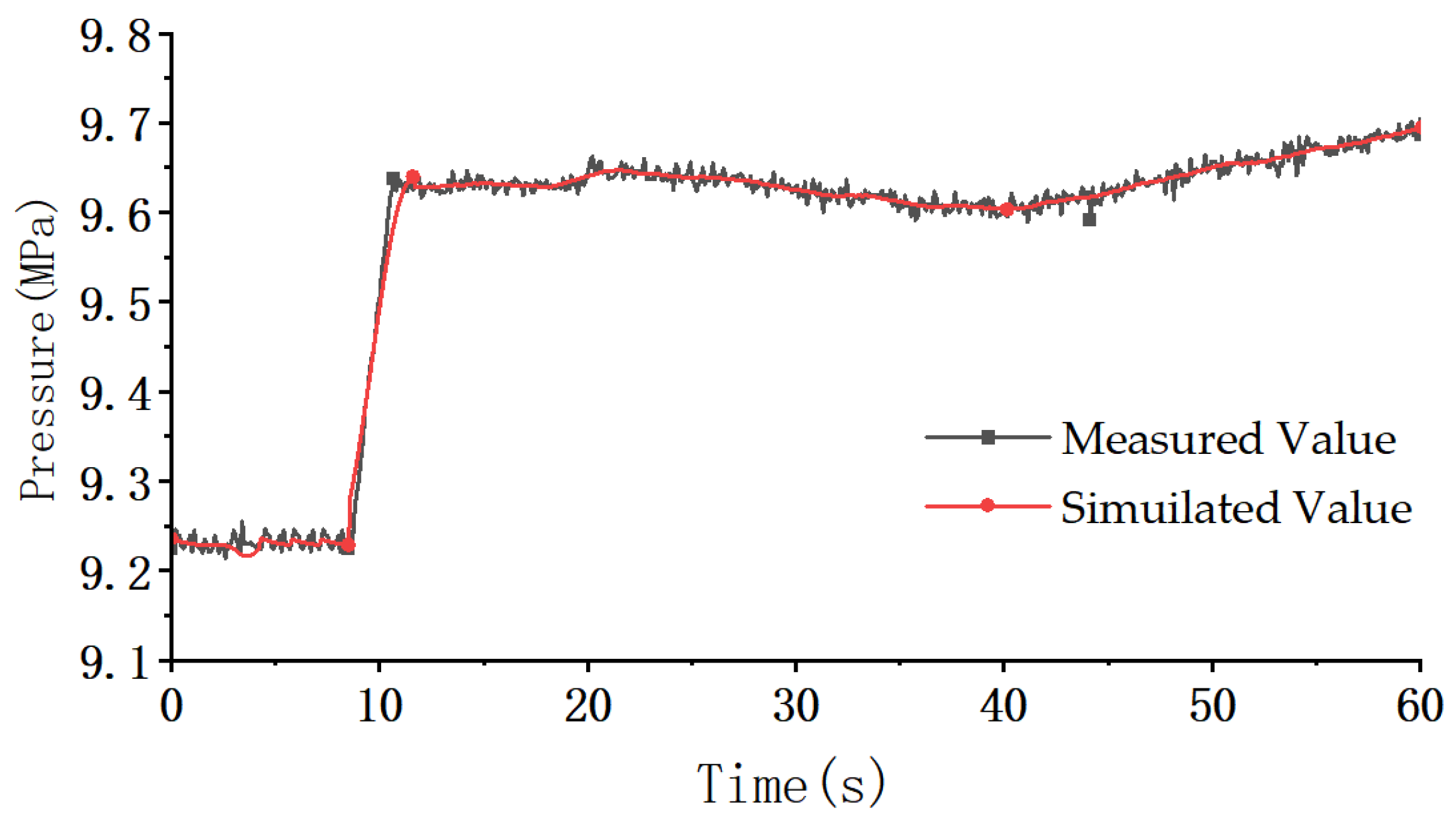
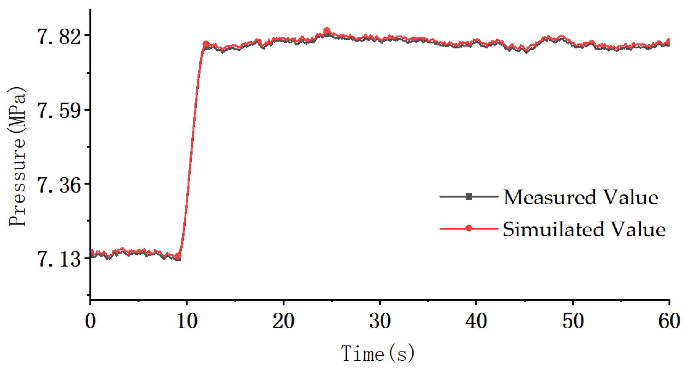
The identified TCH is input into the model to simulate the curve of the governing stage pressure, which is compared with the measured pressure curve of the governing stage as shown in Figure 14.
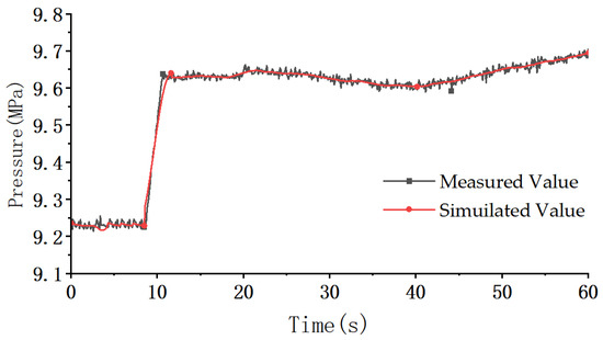
Figure 14.
The curves of the governing stage pressure.
The fitting degree between the simulated and measured curves could be analyzed by . When is greater than 0.8, it indicates that the fitting degree of the curve is higher. of the curve of the governing stage pressure in Figure 14 is 0.967, which again verifies that the algorithm has high identification accuracy.
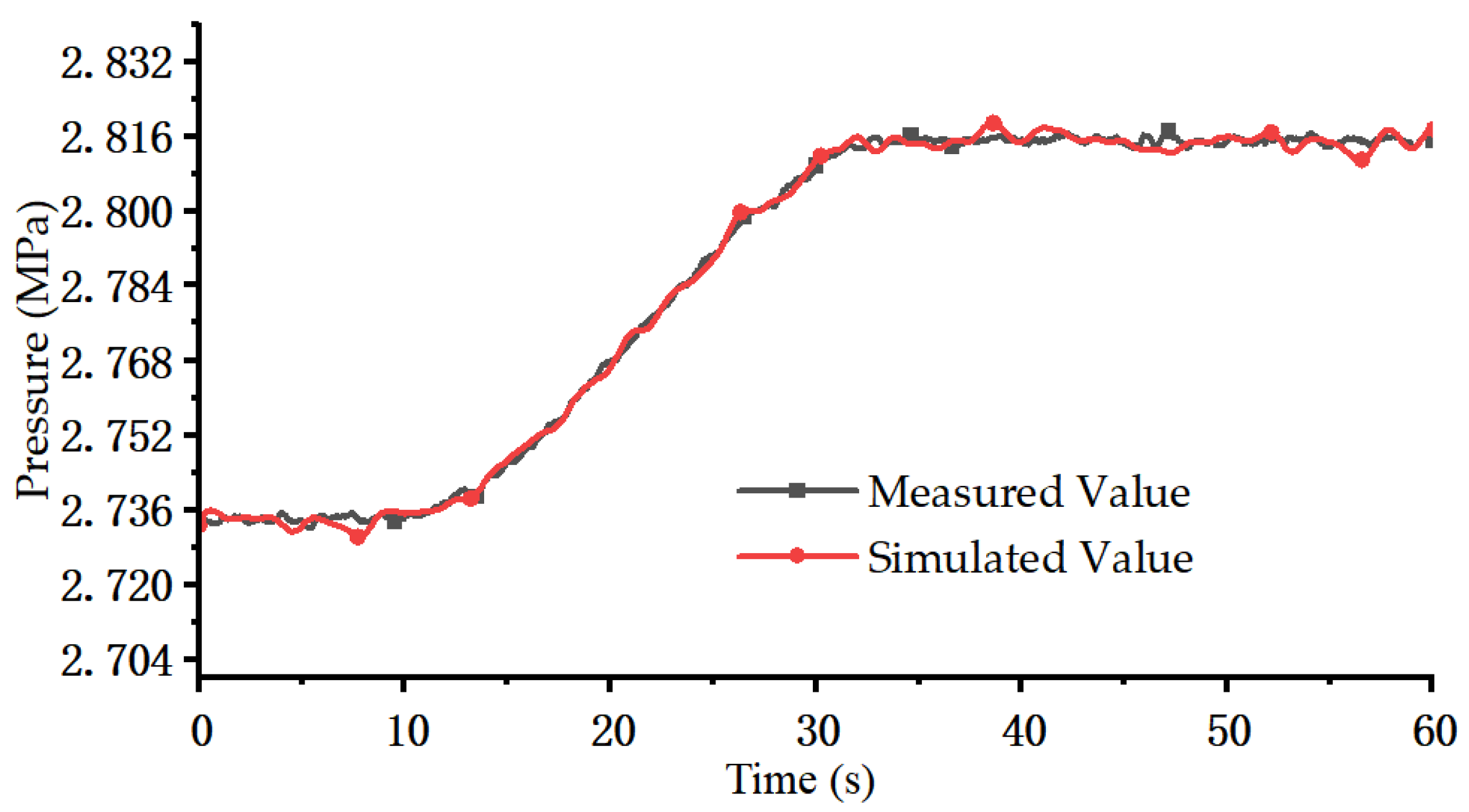
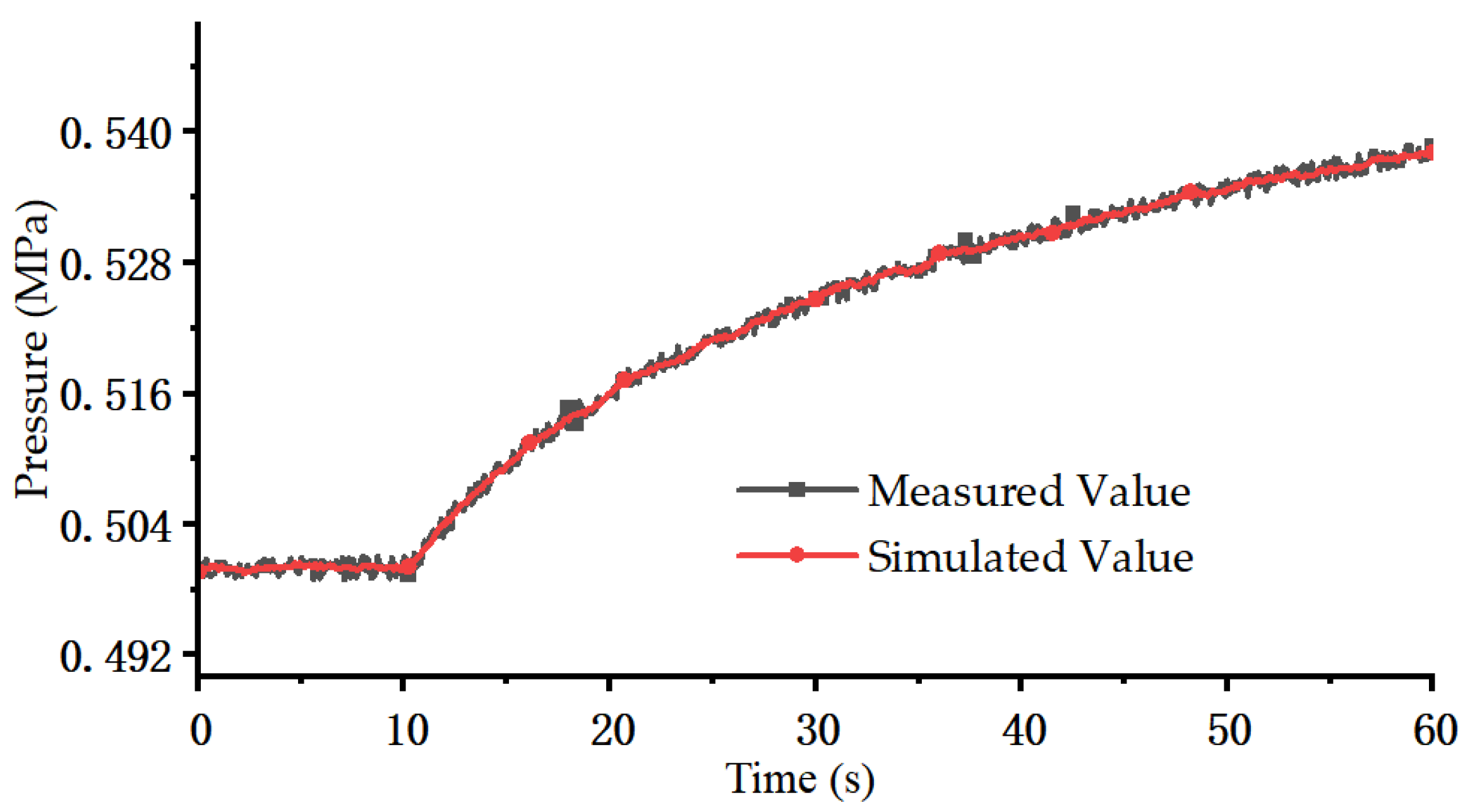
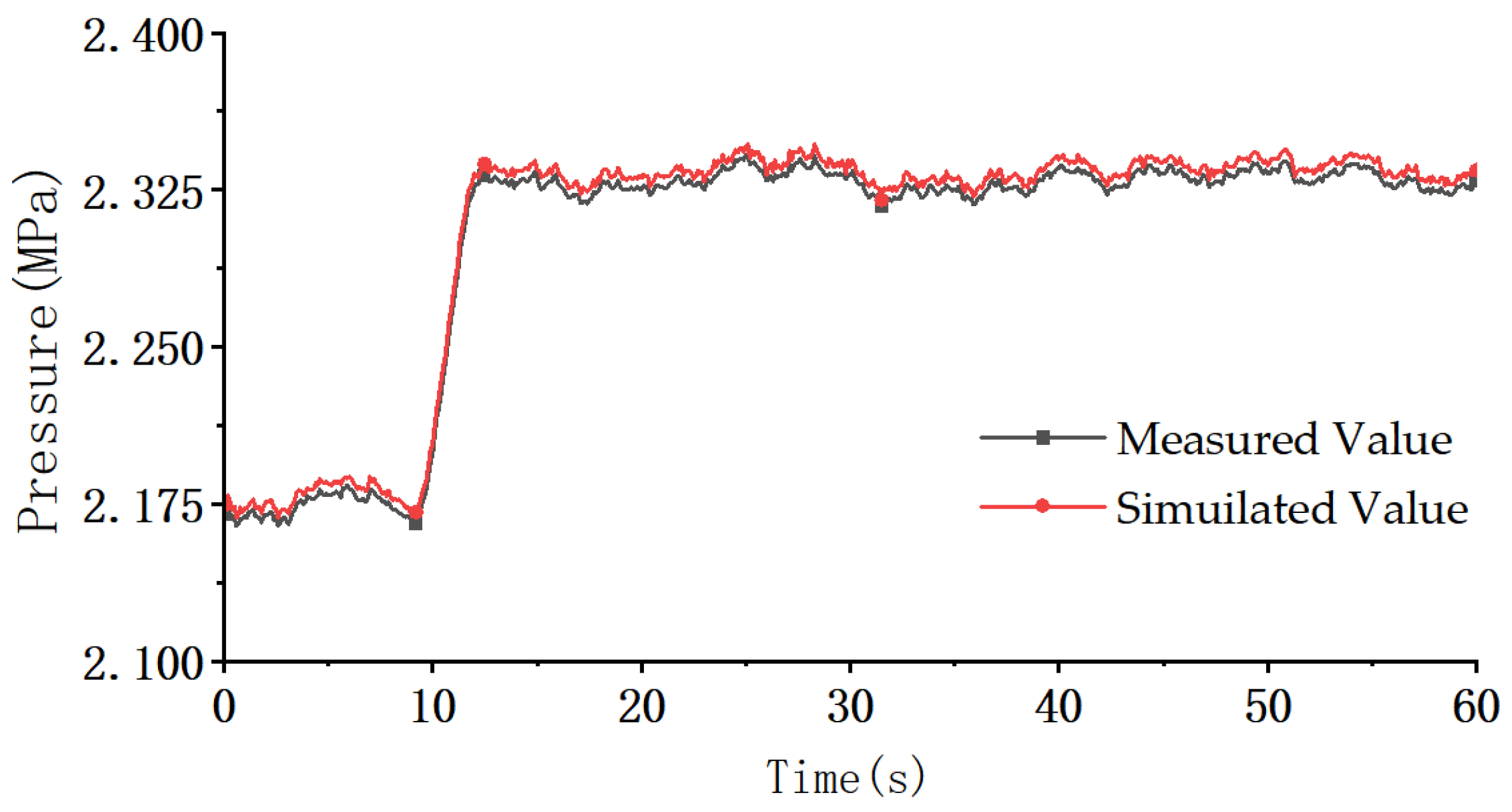
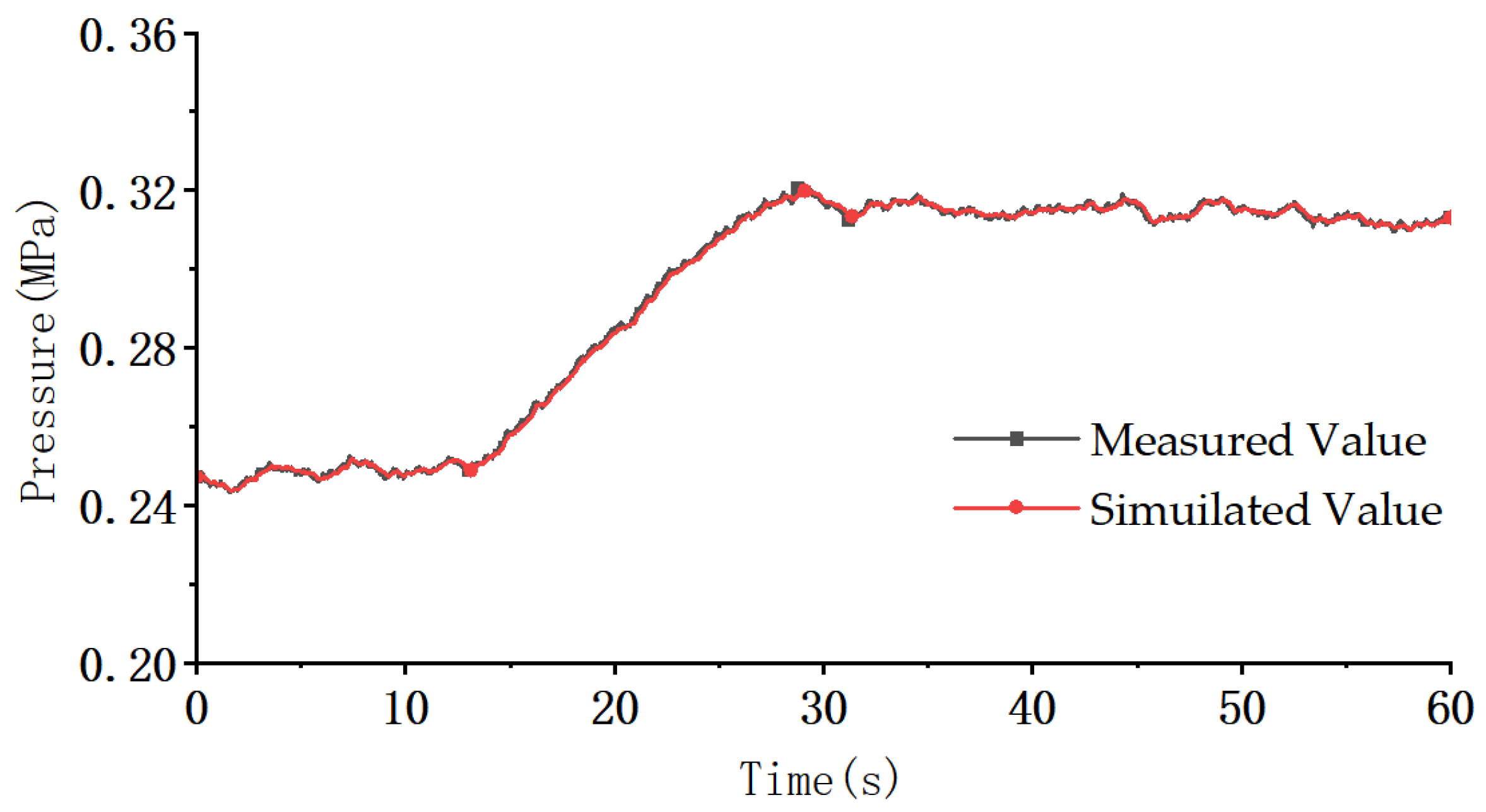
Similarly, the identified TRH is 8.988 s, TCO is 1.002 s, and the simulated and measured curves of reheated steam pressure and low-pressure cylinder inlet pressure are shown in Figure 15 and Figure 16. The calculated are 0.943 and 0.971, both greater than 0.8. The simulation results of various pressures are in good agreement with the measured results, indicating that IBO-WOA has high accuracy and can be applied to practical engineering.
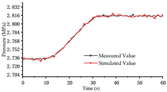
Figure 15.
The curves of reheated steam pressure.
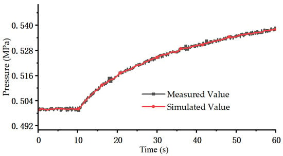
Figure 16.
The curves of low-pressure cylinder inlet pressure.
3.3.2. Experimental Condition 2
The TCH identification curve during the identification process is shown in Figure 17. It can be seen that the identification results of the five algorithms are relatively close. Taking IBO-WOA as the standard, after 11 iterations, it tends to be stable, and the final identification result of TCH is 0.205 s.
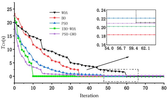
Figure 17.
TCH identification curves of five methods.
The identified TCH is input into the model to simulate the curve of the governing stage pressure, which is compared with the measured pressure curve of the governing stage as shown in Figure 18. between the simulated and measured curves is 0.955, which again verifies that the algorithm has high identification accuracy.
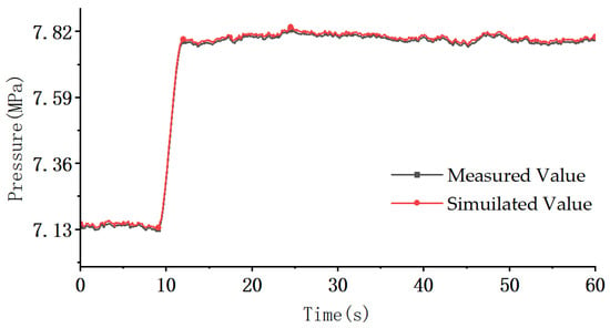
Figure 18.
The curves of the governing stage pressure.
Similarly, the identified TRH is 8.992 s, TCO is 1.005 s, and the simulated and measured curves of reheated steam pressure and low-pressure cylinder inlet pressure are shown in Figure 19 and Figure 20. The calculated are 0.939 and 0.969. The simulation results of various pressures are in good agreement with the measured results.
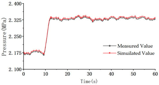
Figure 19.
The curves of reheated steam pressure.
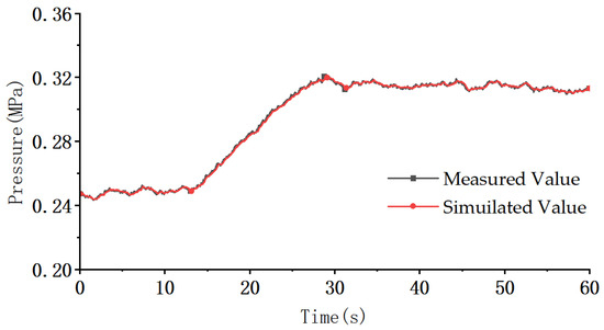
Figure 20.
The curves of low-pressure cylinder inlet pressure.
The identification results of a steam turbine under two experimental conditions are shown in Table 6. According to the table, although there is a significant difference between the two experimental conditions, their identification results are very close, proving that IBO-WOA has good generalization ability and adaptability.

Table 6.
Identification results of a steam turbine under two experimental conditions.
3.4. PFR Simulation Analysis
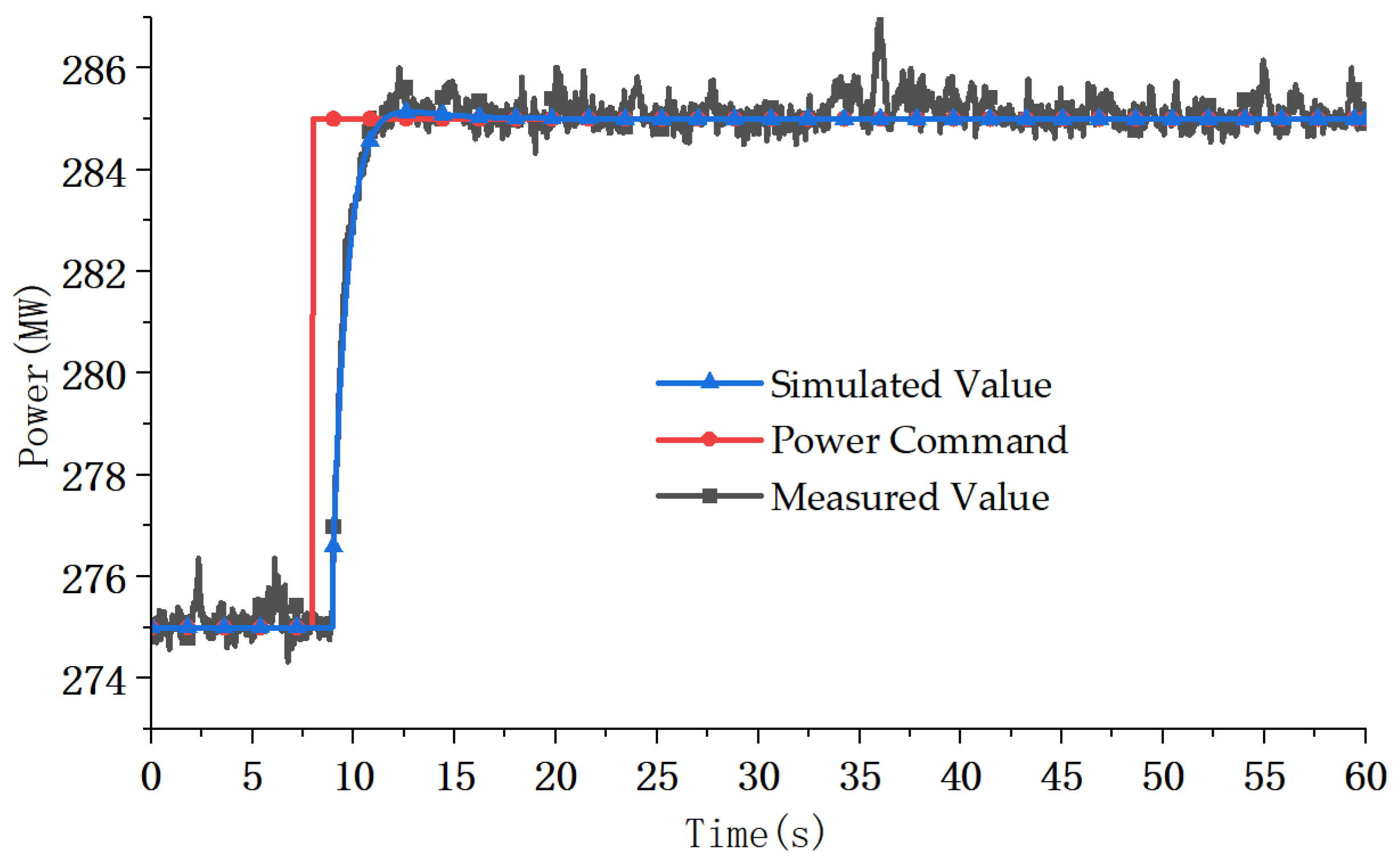
Taking experimental condition 1 as an example, the above parameter identification results are substituted into the PFR model in Figure 3, and simulation verification is carried out for the PFR test. The obtained power simulation curve and measured curve are shown in Figure 21.

Figure 21.
Unit power curves during PFR process.
It can be seen that: the power simulation curve tracks the measured curve well and is closer to the PFR power command curve than the measured curve. After 20 s, the steady-state fluctuation range of the simulated power is reduced to ±0.133 MW, with an overshoot of only 1.33% and no power oscillation throughout the entire process. It indicates that the parameter identification results obtained by IBO-WOA have high accuracy and can be used for the analysis of the PFR response characteristics of actual units. At the same time, it also verifies the feasibility of IBO-WOA in solving power regulation lag and overshoot problems in strongly nonlinear grid systems.
In summary, IBO-WOA can maintain good stability and convergence in complex high-dimensional and noisy environments, and its theoretical basis lies in:
(1) Adaptive control of the search range. In high-dimensional spaces, to prevent the algorithm from converging prematurely to local optima, the hyperparameters of the Gaussian model are optimized by maximizing the marginal log-likelihood function, which can best fit the observation distribution of the objective function, improving the identification accuracy and generalization ability.
(2) Implementation of a repeated evaluation mechanism. In noisy environments, to reduce the impact of noise on the final result, we use a reverse guidance selection mechanism to generate reverse solutions for IWOA outputs, calculate the fitness of both the optimal and reverse solutions, and use the better one as input to IBO, thereby updating the initial training set and completing a closed-loop process for reverse learning feedback. This increases the algorithm’s resistance to noise.
(3) Diversity maintenance strategy. To ensure diversity during the algorithm’s iterations and avoid local optima, the Levy flight mechanism and nonlinear convergence factors are introduced in IWOA to prevent the algorithm from prematurely clustering in high-dimensional search spaces, allowing exploration of a broader optimization space.
4. Conclusions
In the context of building a new-type power system, accurate identification of PFR parameters for a steam turbine is crucial for ensuring grid stability. Conventional identification methods often suffer from issues like getting trapped in local optima and insufficient convergence accuracy. To address these, this paper proposed a hybrid identification method that integrated IBO with IWOA. The proposed approach demonstrated effectiveness through rigorous verification and practical application across nine standard test functions and a 330 MW steam turbine, with comparative analyses against PSO, WOA, BO, and PSO-GWO algorithms. Main conclusions include:
(1) By initializing the Bayesian parameter population using Tent chaotic mapping and the reverse learning strategy, employing a radial basis kernel function hyperparameter training mechanism based on the Adam optimizer, and optimizing the EI function using the L-BFGS-B method, IBO was proposed. By introducing a nonlinear convergence factor and the adaptive Levy flight perturbation strategy, IWOA was proposed. By using the reverse-guided optimization mechanism, three-layer collaborative architecture was constructed: “Bayesian global guidance-WOA local optimization-reverse learning feedback.” which significantly improved global search capability and convergence speed during the identification process, while maintaining high parameter recognition accuracy and robustness.
(2) Through validation on nine standard test functions, including three types of each of the unimodal functions, non-fixed-dimensional multi-modal functions, and fixed-dimensional multi-modal functions, this study demonstrated the superiority of IBO-WOA. Comparative analysis with PSO, WOA, BO, and PSO-GWO showed that IBO-WOA outperformed the other four in optimal values, average values, and standard deviations. The optimization process of IBO-WOA was similar to a straight line approaching the optimal value, which proved that IBO-WOA had better global search ability and local optimal area escape ability, and its identification results had higher accuracy.
(3) Taking PID parameter identification in the electro-hydraulic servo system of a 330 MW steam turbine as an example, this study demonstrated the feasibility and superiority of IBO-WOA through simulated validation using known parameters. During the parameter identification process, IBO-WOA achieved stability after 19 iterations, ultimately yielding identification results with 0.022% relative error. Compared to PSO, WOA, BO and PSO-GWO, IBO-WOA required the fewest iterations to reach stable performance, exhibited the smallest relative error in final identification results, and demonstrated the highest precision. Meanwhile, OOD Test based on noise injection had demonstrated that IBO-WOA had good robustness.
(4) IBO-WOA was employed to identify the time constants of a steam turbine under two experimental conditions, and their identification results were very similar, proving that IBO-WOA had good generalization ability and adaptability. Under experimental condition 1, the identified TCH was 0.202 s, TRH was 8.988 s, and TCO was 1.002 s. The simulation curves and measured curves of governing stage pressure, reheat steam pressure, and low-pressure cylinder inlet steam pressure were well matched. By substituting the identification results of the unit parameters into the PFR model, simulation verification was carried out for the PFR test. The obtained generator power simulation curve can track the measured curve well, proving that the accuracy of IBO-WOA was high and could be used for the analysis of the response characteristics of the actual PFR.
This article proposed IBO-WOA for identifying PFR parameters of a steam turbine, but there are still some shortcomings that need further improvement in future research:
(1) IBO-WOA was only compared with four algorithms—PSO, WOA, BO, and PSO-GWO—initially demonstrating its effectiveness. However, given the vast family of intelligent algorithms, its comparative scope remains insufficient. In the future, a unified test platform should be established to compare IBO-WOA with various advanced and classical algorithms, including GA, Bat Algorithm (BA), and Sparrow Search Algorithm (SSA), etc. This would enable a quantitative evaluation of differences in key metrics such as convergence accuracy, robustness, parameter sensitivity, and computational efficiency, thereby clarifying its optimal application scenarios and areas for improvement.
(2) IBO-WOA has demonstrated potential in PFR parameter identification for 330 MW units, but its industrial-scale application remains constrained by limitations in universal applicability. Given the fundamental differences in control logic and dynamic characteristics between 330 MW turbines and high-capacity turbines, future research urgently needs to analyze the complex mechanisms of their large inertia and multi-loop coupling, thereby driving the targeted evolution of IBO-WOA—for instance, designing adaptive search strategies tailored to high-dimensional parameter spaces. Furthermore, exploring the transfer potential of IBO-WOA to the rapid-response domain of gas turbines requires addressing key challenges. These include strong nonlinearities and noise interference caused by faster load response speeds, higher exhaust temperature fluctuations, and precise fuel valve control in gas turbines. The ultimate goal is to establish a unified modeling and identification framework suitable for fast dynamic processes.
Author Contributions
Conceptualization, W.L., W.H. and C.H.; methodology, S.W. and Y.J.; software, Y.J. and J.S.; validation, W.L., S.W. and C.H.; data curation, W.L., W.H. and Y.J.; writing—original draft preparation, S.W. and J.S.; writing—review and editing, J.S. and C.H.; supervision, W.L.; project administration, W.H. All authors have read and agreed to the published version of the manuscript.
Funding
This research received no external funding.
Data Availability Statement
The original data presented in this study are openly available at https://doi.org/10.5281/zenodo.17395114.
Conflicts of Interest
Authors Wei Li and Weizhen Hou was employed by the company Shandong Electric Power Engineering Consulting Institute Co., Ltd. The remaining authors declare that the research was conducted in the absence of any commercial or financial relationships that could be construed as a potential conflict of interest.
Abbreviations
The following abbreviations are used in this manuscript:
| BO | Bayesian Optimization |
| IBO | Improved Bayesian Optimization |
| WOA | Whale Optimization Algorithm |
| IWOA | Improved Whale Optimization Algorithm |
| IBO-WOA | Improved Bayesian Optimization-Whale Optimization Algorithm |
| PSO | Particle Swarm Optimization |
| PFR | Primary Frequency Regulation |
| L-BFGS-B | Limited-memory Broyden-Fletcher-Goldfarb-Shanno with Bounds |
| DEH | Digital Electro-Hydraulic |
| GA | Genetic Algorithms |
| SA | Simulated Annealing |
| BA | Bat Algorithm |
| SSA | Sparrow Search Algorithm |
| GWO | Grey Wolf Optimizer |
| GP | Gaussian process |
| EI | Expected Improvement |
| PID | Proportional Integral Derivative |
| OOD | Out-Of-Distribution |
References
- Kang, J.Q.; Chen, X.F.; Yang, Z.Y.; Liu, L.; You, M.; Zhao, Y.Z.; Liang, B.Y.; Hao, J.H.; Hong, F. Performance enhancement and optimization of primary frequency regulation of coal-fired units under boundary conditions. Energy Sci. Eng. 2024, 12, 2209–2219. [Google Scholar] [CrossRef]
- Chen, C.; Liu, M.; Li, M.; Wang, Y.; Wang, C. Digital twin modeling and operation optimization of the steam turbine system of thermal power plants. Energy 2021, 290, 129969. [Google Scholar] [CrossRef]
- Zhou, J.; Deng, K.; Wang, H.; Peng, Z. Inexact riemannian gradient descent method for nonconvex optimization with strong convergence. J. Sci. Comput. 2025, 103, 96. [Google Scholar] [CrossRef]
- Yin, H.; Wei, Y.F.; Zhang, Y.J.; Jing, P.P.; Cai, D.Y.; Liu, X.M. Identification of control parameters of the permanent magnetic synchronous generator using least square method. Energy Rep. 2022, 8, 1538–1545. [Google Scholar] [CrossRef]
- Xiang, X.C.; Diao, R.S.; Bernadin, S.; Foo, S.Y.; Sun, F.Y.; Ogundana, A.S. An intelligent parameter identification method of DFIG systems using hybrid particle swarm optimization and reinforcement learning. IEEE Access 2024, 12, 44080–44090. [Google Scholar] [CrossRef]
- Rafei, T.; Yousfi, S.N.; Chrenko, D. Genetic algorithm and Taguchi method: An approach for better Li-Ion cell model parameter identification. Batteries 2023, 9, 72. [Google Scholar] [CrossRef]
- Zhang, Y.; Zhang, C.; Cheng, Z. Parameter identification based on chaotic map simulated annealing genetic algorithm for PMSWG. Prog. Electromagn. Res. M 2022, 113, 59–71. [Google Scholar] [CrossRef]
- Huang, W.K.; Wang, Y.; Hu, H.F.; Xiao, B.H.; Bian, Z.F.; Li, A.; Pan, M.H.; Yang, Y.M. Parameters identification of blade vibration based on dual-sensor full waveform and improved grey wolf optimizer algorithm. Mech. Syst. Signal Process. 2025, 239, 113275. [Google Scholar] [CrossRef]
- Braik, M.; Awadallah, M.; AlBetar, M.A.; AlHiary, H. Enhanced whale optimization algorithm-based modeling and simulation analysis for industrial system parameter identification. J. Supercomput. 2023, 79, 14489–14544. [Google Scholar] [CrossRef]
- Xu, Y.; Mi, L.; Korkali, M.; Chen, X. An adaptive Bayesian parameter estimation of a synchronous generator under gross errors. IEEE Trans. Ind. Inf. 2020, 16, 5088–5098. [Google Scholar] [CrossRef]
- Tang, M.N.; Wang, W.J.; Yan, Y.G.; Zhang, Y.Q.; An, B. Robust model predictive control of wind turbines based on Bayesian parameter self-optimization. Front. Energy Res. 2023, 11, 1306167. [Google Scholar] [CrossRef]
- Shaheenh, I.; Zuo, Y.; Yang, B. Optimized resource allocation in autonomous microgrids through Dual-Level energy management using WOA and game theory. Sustain. Energy Technol. Assess. 2025, 82, 104503. [Google Scholar] [CrossRef]
- Li, Y.T.; Zeng, Y.; Qian, J.; Yang, F.J.; Xie, S.H. Parameter identification of DFIG converter control system based on WOA. Energies 2023, 16, 2618. [Google Scholar] [CrossRef]
- Mammeri, E.; Ahriche, A.; Necaibia, A.; Bouraiou, A.; Mekhilef, S.; Dabou, R.; Ziane, A. An enhanced battery model using a hybrid genetic algorithm and particle swarm optimization. Electr. Eng. 2023, 105, 4525–4548. [Google Scholar] [CrossRef]
- Yousri, D.A.; AbdelAty, A.M.; Said, L.A.; Elwakil, A.S.; Maundy, B.; Radwan, A.G. Parameter identification of fractional-order chaotic systems using different Meta-heuristic Optimization Algorithms. Nonlinear Dyn. 2019, 95, 2491–2542. [Google Scholar] [CrossRef]
- Obadina, O.O.; Thaha, M.A.; Althoefer, K.; Shaheed, M.H. Dynamic characterization of a master-slave robotic manipulator using a hybrid grey wolf-whale optimization algorithm. J. Vib. Control. 2022, 28, 1992–2003. [Google Scholar] [CrossRef]
- Hu, B.; Liu, C.; Yang, Y.; Wang, B.; Cai, D.; Xu, W.F. Adaptive internal model control of SCR denitration system based on multi-objective optimization. IEEE Access 2022, 10, 24769–24785. [Google Scholar] [CrossRef]
- Jiang, J.H.; Xu, C.Z.; An, H.X. Research on the effect of wind turbine bearing fault diagnosis method based on multi-feature calculation and Bayesian optimized machine learning method. Int. J. Interact. Des. Manuf. 2023, 17, 2687–2697. [Google Scholar] [CrossRef]
- Wang, B.C.; He, Y.B.; Liu, J.; Luo, B. Fast parameter identification of lithium-ion batteries via classification model-assisted Bayesian optimization. Energy 2024, 288, 129667. [Google Scholar] [CrossRef]
- Li, C.P.; Wang, X.H.; Duan, L.C.; Lei, B. Study on a discharge circuit prediction model of High-Voltage Electro-Pulse boring based on Bayesian fusion. Energies 2022, 15, 3824. [Google Scholar] [CrossRef]
- Guo, Q.; Gao, L.; Chu, X.J.; Sun, H.D. Parameter identification for Static Var compensator model using sensitivity analysis and improved whale optimization algorithm. CSEE J. Power Energy Syst. 2022, 8, 535–547. [Google Scholar] [CrossRef]
- Wang, X.Q.; Deng, L.F.; Zhao, C.; Zhang, W.Q. WOA-based parameter adaptive VMD combined with wavelet thresholding for bearing fault feature extraction. J. Nondestruct. Eval. 2025, 44, 74. [Google Scholar] [CrossRef]
Disclaimer/Publisher’s Note: The statements, opinions and data contained in all publications are solely those of the individual author(s) and contributor(s) and not of MDPI and/or the editor(s). MDPI and/or the editor(s) disclaim responsibility for any injury to people or property resulting from any ideas, methods, instructions or products referred to in the content. |
© 2025 by the authors. Licensee MDPI, Basel, Switzerland. This article is an open access article distributed under the terms and conditions of the Creative Commons Attribution (CC BY) license (https://creativecommons.org/licenses/by/4.0/).

