Article

Instance-Based Transfer Learning-Improved Battery State-of-Health Estimation with Self-Attention Mechanism

1
School of Automation Engineering, University of Electronic Science and Technology of China, Chengdu 611731, China
2
AVIC Chengdu Aircraft Design & Research Institute, Chengdu 610091, China
3
Aviation Key Laboratory of Science and Technology on Aerospace Vehicle, Chengdu 610091, China
*
Authors to whom correspondence should be addressed.
Energies 2025, 18(21), 5672; https://doi.org/10.3390/en18215672
Submission received: 9 September 2025 / Revised: 16 October 2025 / Accepted: 27 October 2025 / Published: 29 October 2025

Abstract

Batteries’ state-of-health (SOH) estimation has attracted appealing attention in energy industrial systems. In conventional data-driven methods, the lack of target data and different source data can also lead to poor model training effect. To tackle this problem, this paper combines the instance-based transfer (ITL) and interpretable self-attention mechanism (SAM) to integrate the fitting ability of long short-term memory (LSTM), which can improve the SOH estimation performance. ITL re-weights the temporal instance of a training set to give more impact of target-like data, which can relax the independent and identical distribution (IID) assumption. SAM method can enhance the estimation performance by re-weighting the spatial features, and be interpreted by detailed visualization. During the model training, the pre-trained multi-layer LSTM model is fine-tuned by target data to make full use of target information. The proposed method has outperformed other compared algorithms in transfer tasks, and has tested in real-world cross-domain conditions datasets.

1. Introduction

Developing new and sustainable energy represents a critical strategy to address mounting environmental and energy pressures. Lithium-ion batteries (LIBs), valued for their long lifetime and high energy density, have found widespread application across numerous domains and now serve as a primary energy storage solution [1,2]. These advantages have further propelled the adoption of LIBs in electric vehicles, mobile devices, aerospace, and other sectors [3]. However, the rapid proliferation of batteries has concurrently heightened potential risks within industrial systems. Beyond batteries, fault diagnosis in renewable energy systems has also progressed from heuristics to data-driven and intelligent paradigms [4]. When LIBs age and fail, they can trigger fires and explosions, constituting a major source of accidents in industrial settings. Therefore, prognostics and health management (PHM) for batteries in large-scale industries is crucial for real-world operational safety [5,6]. The battery management system (BMS) estimates the SOH using various models to ensure batteries operate within safe limits [7]. SOH estimation is also a key indicator for predicting remaining useful life, diagnosing faults, and other critical functions. Consequently, achieving accurate SOH estimation is essential. Generally, the SOH value is defined as the ratio between the current capacity and the initial capacity. An initial SOH value of 100% is typically assigned, which decreases during the aging process [8]. While direct measurements—such as internal resistance, capacity, and impedance—can accurately determine the current SOH value, these methods are unsuitable for online estimation during battery operation. Consequently, indirect SOH estimation techniques have become significant, primarily categorized into model-based and data-driven approaches [9]. On the model-based side, recent electrochemical–thermal coupling studies emphasize low-temperature degradation with real-time coefficient correction to improve SOC/SOH tracking fidelity [10]. Within the data-driven branch, combining incremental-capacity (ICA) features with improved LSTM architectures has proved effective on multiform Li–S batteries [11]. Model-based approaches analyze internal electrical and chemical mechanisms to construct equivalent circuits and mathematical models. These methods offer advantages in intuitiveness and interpretability [12]. However, due to the inherent complexity and intractability of battery modeling, developing a generalized physical model-based method remains challenging [13]. Data-driven approaches are further divided into statistical learning and machine learning methods. Statistical learning methods, such as Support Vector Machines (SVM) and Relevance Vector Machines (RVM), focus on identifying correlations between input variables using kernel-based methods or matrix transformations. For instance, Guo et al. developed an RVM-based capacity estimation model aided by principal component analysis [14]. Nevertheless, these methods often require large sample sizes, posing challenges for model training efficiency and computational time. The rise of machine learning, particularly deep learning, offers new possibilities for mining internal data patterns and enhancing SOH estimation [15]. Machine learning emphasizes learning complex mapping functions to optimize performance [16]. Chang et al., for example, proposed a genetic algorithm-based wavelet neural network for SOH estimation [17]. For time-series data characteristic of battery degradation, Recurrent Neural Networks (RNNs) have shown significant promise. Choi et al. utilized a long short-term memory (LSTM) network to extract information from multi-channel charging profiles, achieving accurate SOH estimation [18]. Similarly, Li et al. proposed a variant LSTM model designed for more robust SOH estimation [19].
The dependency of data-driven methods on extensive data makes it challenging to establish complex, nonlinear mapping functions and achieve accurate SOH estimation under small-sample conditions. To address this limitation, similar large-scale laboratory battery data from other sources (source domain) can be utilized to augment model training, supplementing the limited real-world target domain data. However, this approach introduces new challenges. The data distributions between the source and target domains are typically different, violating the IID assumption crucial for guaranteeing the effectiveness of standard machine learning models. This distribution discrepancy, or domain shift, means that directly transferring knowledge from the source to the target domain can lead to negative transfer [20], a major source of error in model training. Transfer learning has been proposed to relax the IID assumption in such scenarios [21,22]. For SOH estimation, a common challenge arises when the source datasets originate from multiple operating conditions, causing significant domain shift. Models trained directly on such diverse source data often perform poorly when deployed online in a specific target condition. Transfer learning methods for SOH estimation can be categorized into four main types based on the nature of the transferred knowledge: instance-based, feature-based, model-based, and relational-based [23]. Instance-based methods focus on assigning higher weights to source domain samples deemed more similar to the target domain. Feature-based methods aim to learn a new, domain-invariant feature representation that enhances model training. This is a highly active research area. For example, Qin et al. proposed a transferable LSTM model incorporating multi-stage domain-invariant representation learning [24]. Li et al. designed a kernel ridge regression model based on semi-supervised transfer component analysis for accurate SOH prediction [25]. Ye et al. introduced a domain adversarial transfer learning approach to achieve invariant representation for SOH estimation [26]. Model-based methods leverage shared parameters or model structures learned from the source domain to aid training on the few-sample target dataset. Deng et al., for instance, employed a pre-trained LSTM model for SOH estimation by recognizing degradation patterns [27]. Relational-based transfer learning leverages the underlying relationships, structures, and rules from the source domain, rather than superficial data or features, by identifying and adapting them to the target domain for effective knowledge transfer [28]. Numerous studies focus on minimizing distribution divergence through domain-invariant representation learning [29]. Nevertheless, identifying the optimal representation, particularly under multiple operating conditions, remains difficult, and the risk of negative transfer persists. Furthermore, within datasets, individual instances and data points inherently possess varying levels of importance. Accurately assigning weights to these temporal and spatial instances is therefore critical. This underscores the strong motivation for research into battery SOH estimation under multi-source domain conditions.
  • To eliminate dependence on prior knowledge, it is crucial to develop accurate data-driven methods for battery SOH estimation.
  • Comprehensive importance weighting is essential for SOH estimation under multiple complex operating conditions to effectively extract useful information.
  • Conducting interpretability analysis of the operational mechanisms within black-box data-driven methods can enhance credibility and provide clearer guidance for battery management system maintenance.
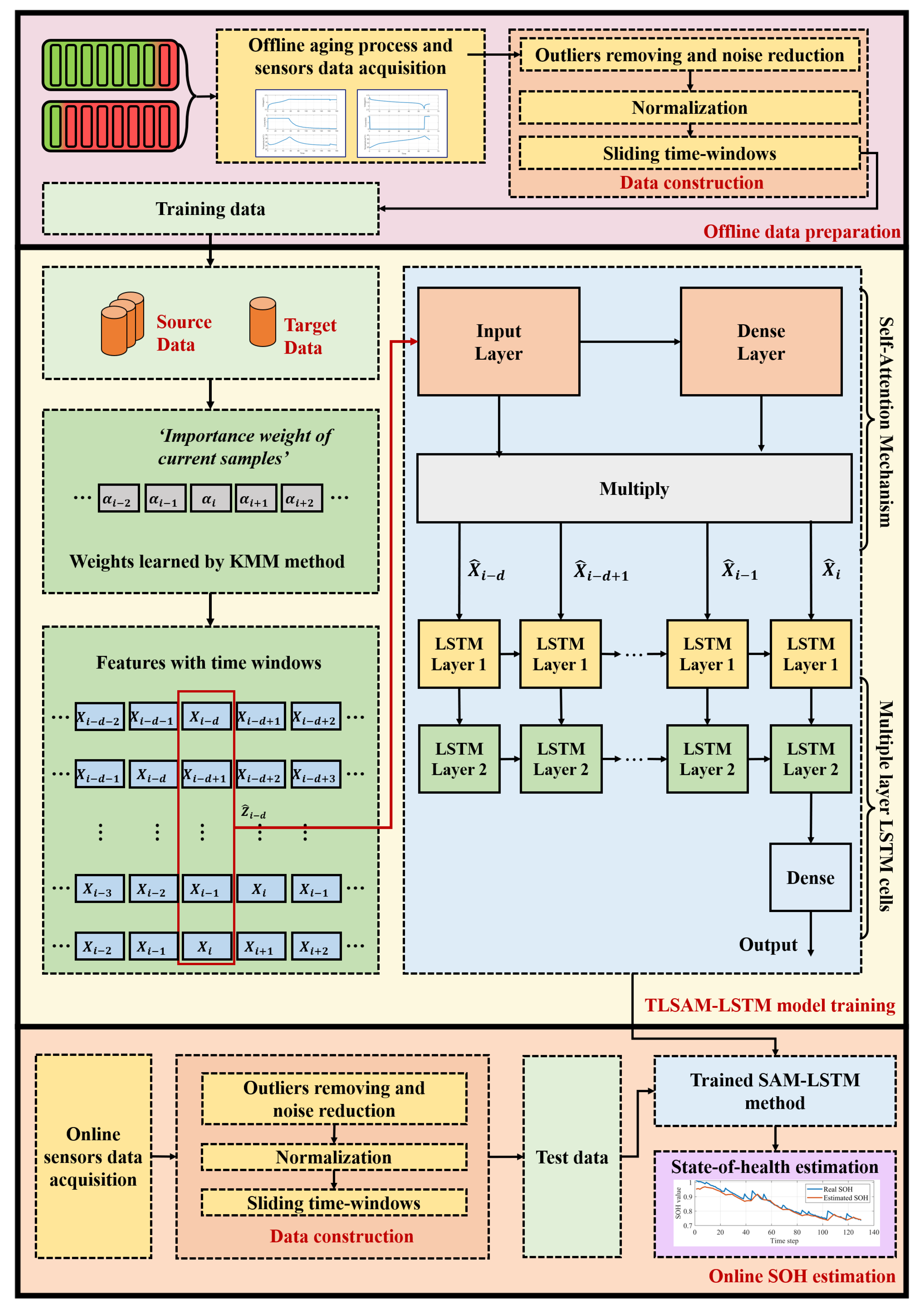
Based on the above motivation, we propose a comprehensive importance weighting-based method for battery SOH estimation to fully extract information from multi-source datasets. The SOH estimation process comprises offline training and online testing phases. Data-driven methods leverage sensor data to extract useful information, training models on large-scale historical data. These models then generate accurate predictions using real-time sensor data during online deployment (Figure 1).
Fundamentally, battery SOH estimation constitutes a regression problem. Let X denote input data from the feature space and Y represent the output SOH value. Given a dataset D = { ( X i , Y i ) } i = 1 N , where X i X (original feature space), Y i Y (label space), and N is the total sample count. To capture temporal dependencies in continuous streaming data, we apply a sliding time-window approach with window size d. This transforms the original input X into Z with dimensions m × d per sample. The resulting time-window dataset D = { ( Z i , Y i ) } i = 1 N d + 1 facilitates recurrent model implementation. The mapping function ψ : Z Y , obtained through historical data training, is realized by the TLSAM-LSTM model proposed in this work. Therefore, the contributions of the paper can be concluded as below:
  • This study employs sliding-window-based features to implement a data-driven battery health monitoring framework. Recognizing that each data point in the input matrix contributes differentially to the results, we incorporate feature weighting via a self-attention mechanism.
  • For multi-source domains, data source quality significantly impacts model training outcomes and generalization capability in the target domain. We derive sample weights through a sample transfer approach that minimizes inter-dataset distribution distances, assigning higher weights to highly transferable samples to facilitate domain adaptation [30].
  • Our methodology incorporates dual weighting across feature and sample dimensions. Employing a multi-layer LSTM architecture as the base estimator, we implement pre-training and fine-tuning strategies to effectively capture underlying data relationships and reduce estimation errors.
  • Validation on the CALCE and NASA datasets demonstrates the superior performance of our proposed algorithm in comparative analysis. To enhance interpretability, we develop a visual representation of the importance weighting mechanism, illustrating the model’s focus during the training process.
The remainder of this paper is organized as follows. Section 2 describes the proposed TLSAM-LSTM methodology in detail. Section 3 presents the experimental results and discussions. Finally, Section 4 concludes the paper.

2. Methodology

This section elaborates the proposed TLSAM-LSTM method, with its comprehensive framework depicted in Figure 2. The implementation integrates four core components: (1) temporal instance re-weighting via kernel mean matching (KMM) to adjust sample significance, (2) feature prioritization through a self-attention mechanism that dynamically assigns higher weights to critical spatial features, (3) deployment of long short-term memory (LSTM) networks as the base estimator for SOH prediction, and (4) execution of pre-training with fine-tuning strategies to facilitate cross-domain adaptation. This cohesive architecture enables effective information extraction while ensuring domain transfer robustness.

2.1. Discrepancy-Based Importance Weighting

This work employs KMM to mitigate domain discrepancy between source and target distributions by assigning importance weights to source samples. During training, samples distant from the target domain receive lower weights. We adapt KMM for sliding time-window-based SOH estimation, defining the transformed variable Z ¯ i of dimension 1 × d (Equation (1)), where Z ¯ serves exclusively as an intermediate variable in this subsection:
Z ¯ i = 1 m i = 1 m X i , 1 , , i = 1 m X i , d
Suppose the data Z S with source distribution P S ( Z ¯ ) , and Z T with target distribution P T ( Z ¯ ) . In kernel method, the ψ ( Z ¯ ) is as a mapping function from the finite-dimensional data into high-dimensional space. In KMM, maximum mean discrepancy (MMD) is proposed to describe the distribution distance of source and target domain in the reproducing kernel Hilbert space (RKHS), which means the discrepancy of mathematical expectations E S [ α i ψ ( Z ¯ ) ] and E T [ ψ ( Z ¯ ) ] , as shown in Equation (2):
α * = a r g m i n α E Z ¯ P S [ α i ψ ( Z ¯ ) ] E Z ¯ P T [ ψ ( Z ¯ ) ] H 2 = a r g m i n α 1 m S i = 1 m S α i ψ ( Z ¯ i ) 1 m T j = 1 m T ψ ( Z ¯ j ) H 2
where α i denotes the importance weight of the i-th sample, · H 2 the RKHS 2-norm, and m S , m T the sample counts of source and target domains. Constraints enforce α 0 and | E Z ¯ P S [ α i ] 1 | ϵ for small ϵ > 0 . The radial basis function (RBF) kernel κ ( Z ¯ i , Z ¯ j ) in Equation (2) is given by
κ ( Z ¯ i , Z ¯ j ) = ψ ( Z ¯ i ) · ψ ( Z ¯ j ) = e λ Z ¯ i Z ¯ j 2 .
Importance weights are calculated by minimizing Equation (2), and more clear expression of Equation (2) can be extended as Equation (4):
α * = a r g m i n α 1 m S i = 1 m S α i ψ ( x i ) 1 m T i = 1 m T ψ ( x i ) H 2 = a r g m i n α i = 1 m S j = 1 m S α i α j m S 2 κ ( Z ¯ i , Z ¯ j ) 2 i = 1 m S j = 1 m T α i m S m T κ ( Z ¯ i , Z ¯ j ) + i = 1 m T j = 1 m T 1 m T 2 κ ( Z ¯ i , Z ¯ j ) = a r g m i n α 1 m S 2 α T K α 2 m S m T K 2 T α + c o n s t = a r g m i n α 1 m S 2 α T K α 2 m S 2 K * T α
where α = [ α 1 , , α m S ] T , K with { K | K i , j = κ ( Z ¯ i , Z ¯ j ) } , K 2 with { K 2 | K 2 , ( i , j ) = i = 1 m T κ ( Z ¯ i , Z ¯ j ) } , and K * with { K * | K * , ( i , j ) = m S m T i = 1 m T κ ( Z ¯ i , Z ¯ j ) } . The weight calculation can be converted to a quadratic program, and solved by an optimization procedure.

2.2. Self-Attention-Based Importance Weighting

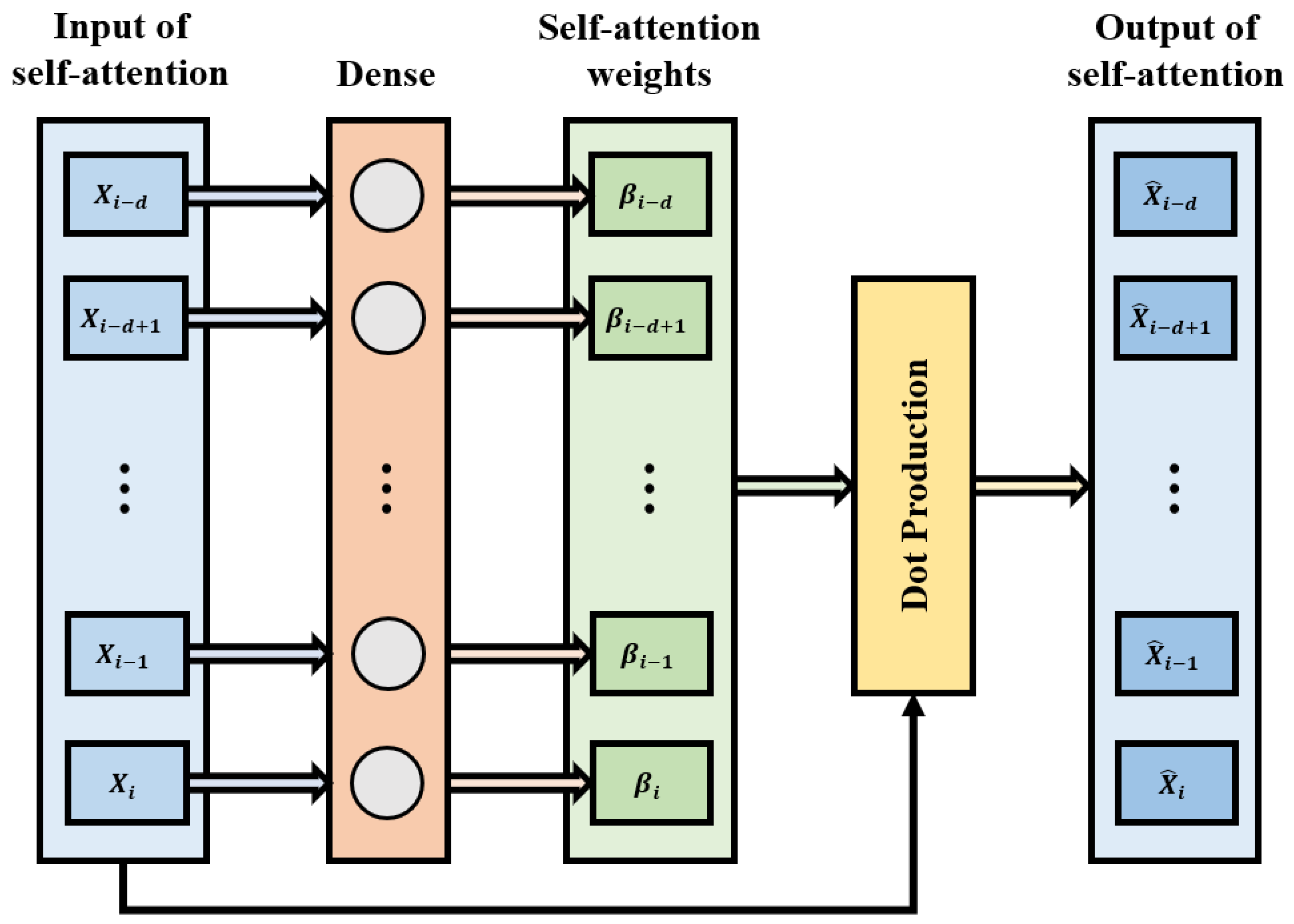
The self-attention mechanism serves as a critical component for assigning temporal and feature weights, enabling enhanced extraction of relevant information from datasets. Following sliding time-window processing, data pairs { Z t , Y t } are obtained at each timestep t during training, where Z t represents a two-dimensional matrix of dimensions m × d (m: sensor dimensions, d: window length). The detailed architecture is illustrated in Figure 3. Given Z i = { x i , 1 ; x i , 2 ; ; x i , d } with x i , j R m , the self-attention layer computes feature importance weights W i through linear transformation x l t = W A x i + b i followed by sigmoid activation:
s i = 1 1 + exp ( x l t )
Temporal weights β i for each window position are then normalized via softmax:
β i = softmax ( s i ) = exp ( s i ) k = 1 d exp ( s k )
The final weighted time-window representation Z ^ i is computed as
Z ^ i = { x ^ i , 1 , x ^ i , 2 , , x ^ i , d } = { β 1 x i , 1 , β 2 x i , 2 , , β d x i , d }

2.3. Training Process

We employ LSTM as the foundational predictor for battery SOH estimation. To leverage multi-source domain data effectively, we implement a pre-training and fine-tuning strategy for high-precision target task performance. The LSTM architecture is detailed in Figure 4, comprising three core gating mechanisms (Equations (8)–(13)):
  • Input gate: determine the useful information to the cell state in the current sequence.
    i t = σ ( W x i x t + W h i h t 1 + b i )
    g t = t a n h ( W x g x t + W h g h t 1 + b g )
  • Forget gate: decide which part of the information is forgotten, and update cell state with input gate.
    f t = σ ( W x f x t + W h f h t 1 + b f )
    c t = f t c t 1 + i t g t
  • Output gate: the state h t 1 , x t , C t are used jointly to determine the current hidden state h t .
    o t = σ ( W x o x t + W h o h t 1 + b o )
    y t = h t = o t t a n h ( c t )
where f t means output of forget gate, aiming at control long-term memory c t retention state. i t is output of input gate, with g t to decide to join long-term memory information. Output gate o t is used to control long-term memory and add it to short-term memory in Equation (13). W x f , W x i , W x o , W x g represents weight connection with input variables and W h f , W h i , W h o , W h g with hidden states (short-term memory). b f , b i , b o , b g are biased terms.

2.4. Pre-Train and Fine-Tuning

Our proposed method also depends on the forward calculation and error back-propagation processes, as shown in Figure 5. During forward calculation, the real expression is set as Equation (14).
Y i = f ( Z i | θ ) = f 2 ( Z ^ i | θ L S T M ) = f 2 ( f 1 ( Z i | θ S A M ) | θ L S T M )
where f represents the proposed TLSAM-LSTM model mapping from Z i to Y i , f 1 and f 2 represent the mapping function of related neural networks, θ S A M and θ L S T M mean the algorithm parameters in brief, and θ is all parameters of the proposed TLSAM-LSTM method.
After forward calculation, loss function is defined as Equation (15) to realize error back-propagation.
L = i = 1 N b a t c h α i Y i p r e d Y i r e a l 2 2 = i = 1 N b a t c h α i f 2 ( f 1 ( Z i | θ S A M ) | θ L S T M ) Y i r e a l 2 2
where weight α is calculated by unsupervised algorithm KMM based on source and target data in Section 3.1, which can assign high weight for similar data. N b a t c h means the mini-batch size of samples, and Y i r e a l and Y i p r e d represent the real and predicted SOH value. The detailed gradient descent of the training process is shown in Equations (16) and (17).
θ S A M T + 1 = θ S A M T λ L θ S A M = θ S A M T λ L f 2 f 2 Z ^ i Z ^ i f 1 f 1 θ S A M
θ L S T M T + 1 = θ L S T M T λ L θ L S T M = θ L S T M T λ L f 2 f 2 θ L S T M
where θ S A M T and θ L S T M T mean the state of parameters θ S A M and θ L S T M at the T time. λ represents learning rate, the format of f 1 / θ S A M and f 2 / θ L S T M consists of a derivative of the activation function and matrix multiplication. The detailed mapping format has been introduced in Section 3.2 and Section 3.3. Adaptive moment estimation (Adam) is used to optimize the gradient descent during training process. For such multi-layers neural networks, there is a general explanation that the shallow layers represent the general features and the deep layers represent the specific features [31]. Under a large amount of source data, there is a learned parameter θ 0 for TLSAM-LSTM model. Then, we can freeze the frontier layers which are almost the same between source and target tasks, and fine-tune the latter layers’ parameters θ as shown in Equation (18).
θ * = arg min θ L ( θ | θ 0 , D t a r g e t )
where L means the loss function of real and estimated value; the pre-trained parameter θ 0 includes θ S A M and the first layer of θ L S T M , and the fine-tuning parameter θ includes the second layer of θ L S T M and the output layer.

2.5. Algorithm Implementation

The main steps of the proposed TLSAM-LSTM model are shown in Algorithm 1. In the proposed method, weight calculation in Section 3.1 and Section 3.2 can let more important instance and features have more impact on results. Furthermore, transfer learning embodies in Section 3.1 and Section 3.4, which can make full use of source information selectively, reduce the negative impact of non-IID influence. LSTM in Section 3.3 can get temporal information from gated structure, and avoid the gradient vanishing and explosion. The above sub-methods can ensure the model can have great estimation performance online.
Algorithm 1: Process of TLSAM-LSTM methods
Energies 18 05672 i001

3. Experimental Results and Improvement Analysis

3.1. Datasets Selection and Preprocessing

3.1.1. Datasets Introduction

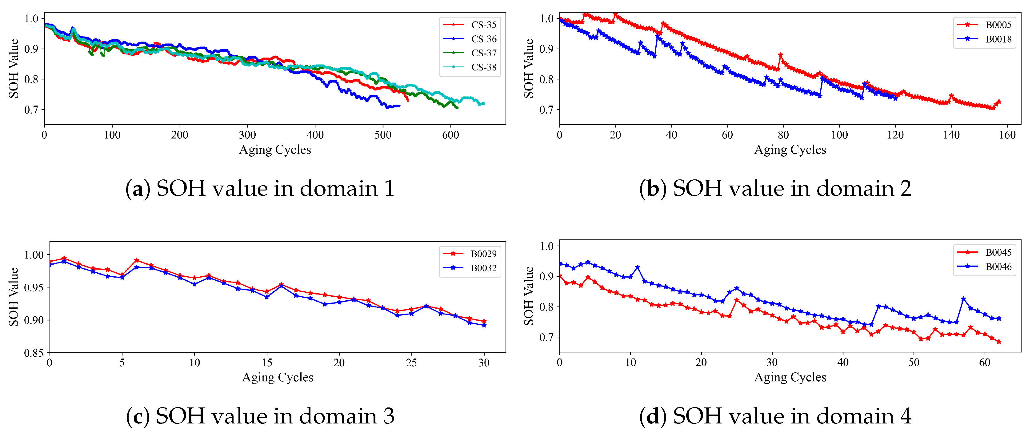
The Center for Advanced Life Cycle Engineering (CALCE) from the university of Maryland has published batteries aging datasets, with the aging process of charging and discharging stages [32]. The detailed parameters of these different domains can be seen in Table 1. The SOH value with aging cycles is shown in Figure 6. First, batteries are charged in the constant current (CC) mode until the voltage reaches 4.2 V, and then charged in the constant voltage (CV) mode until the charging current drops to 20 mA. Then, batteries are discharged in constant current (CC) mode until reaching the drop-out voltage V D r o p . The related rated capacity C R is 1.1 Ahr, which drops to 30% generally when batteries reach the end of life (EOL). Another widely used NASA batteries benchmark is from a real-world experiment [33]. Four similar ‘18650’ battery cells include B05, B06, B07, and B18, which are under a rated capacity around 2 Ahr. There are also other experiments in NASA, including the B29, 30, 31, 32 and the B45, B46, B47, B48 with different operating conditions. The frontier cells are worked in large current I D C , and the latter cells are worked in low ambient temperature T A . For LIBs’ run-to-failure benchmark, this paper uses the CALCE and NASA datasets with four different operating conditions in real-world experiments.

3.1.2. Feature Extraction

In this paper, seven features are selected as model input, which are sampled from CC stage in charging [34]. The detailed instrument is shown in Table 2.

3.1.3. Preprocessing

Data preprocessing is mainly used to remove the adverse impact of useless information in datasets, which is conducive to better experimental estimation effect. Three main parts are proposed here, including the outliers removing, noise reduction, and normalization.
  • Outliers removing: Set σ as the standard deviation of a short time interval. In the short time duration, if any feature value exceeds the 2 σ of average, the related samples are set as an outlier. Outliers are removed to enhance the data quality.
  • Noise reduction: Reduce the negative impact of noise on data quality by moving average method.
  • Normalization: Features are transformed into a range of 0 to 1, which can reduce the impact of real data size imbalance.

3.1.4. Task Setting

In order to validate the batteries’ SOH estimation performance of the proposed method in the cross-domain process, three experimental tasks are designed in this paper. Select domains 2, 3, and 4 with less data as target, and then design three experimental tasks. In a single task, data from other domains are used as source. The specific task setting is shown in the Table 3.

3.2. Compared Algorithms and Hyper-Parameter Settings

Ablation study is used here as compared algorithms to verify the performance of the proposed method. Various machine learning-based methods are used for comparison, as shown below:
  • LSTM-NS (No Source): LSTM model is only trained by few known target datasets.
  • CNN (Source): The Convolutional Neural Network automatically extracts local features from input data through its hierarchical architecture of convolutional, pooling, and fully-connected layers. This architecture progressively compresses information, reduces data redundancy, and ultimately enhances the model’s generalization capability.
  • LSTM-S (Source): Source and target datasets are used to train the LSTM model, but there is no difference during training process.
  • LSTM-PS: LSTM model is pre-trained by source data, and then fine-tuned by target data.
  • TL-LSTM: Without SAM-based method, TL-LSTM combines the subsections A, C, and D in Section 3.
  • SAM-LSTM: Without KMM-based method, SAM-LSTM combines the subsections B, C, and D in Section 3.
  • TLSAM-LSTM: Proposed complete method that is described in Algorithm 1.
Some indicators are used as a standard for performance analysis, including the root mean square error (RMSE) and mean absolute percentage error (MAPE), as shown in Equations (19) and (20) in detail.
I R M S E = 1 N i ( Y ^ i Y i ) 2
I M A P E = 100 % N i Y ^ i Y i Y i
where N means the numbers of samples, and Y ^ i and Y i are the ith predicted and real SOH label. Smaller indicators represent the better performance for estimation. Compared with other metrics, the choice of MAPE and RMSE is primarily driven by their alignment with the core goal of this study, which can achieve accurate and interpretable cross-domain SOH estimation for lithium-ion batteries. As a squared-error-based metric, RMSE is sensitive to large estimation errors (e.g., significant deviations between predicted and real SOH in late battery aging stages). This aligns with our focus on ensuring the model’s reliability in critical scenarios (e.g., avoiding underestimation of SOH that could lead to unexpected battery failure), as it effectively penalizes severe prediction biases. Expressed as a percentage, MAPE offers intuitive interpretability of relative estimation errors. It is particularly valuable for SOH estimation, where stakeholders need to understand error magnitudes relative to the actual SOH value.
Hyper-parameters setting is a key progress in machine learning. Task 1 is taken as an example to demonstrate the optimal hyper-parameters of the proposed TLSAM-LSTM model. In each adjustment, a single variable is controlled to analyze the learning rate, sliding time-windows size, and the layer nodes. The detailed compared results are as shown in Table 4.
Figure 7a,b show the impact of learning rate. By comparison, the learning rate is set to 0.01, which is the best value for model training among the candidate values. Figure 7c,d reflect the impact of sliding time-windows size. The experiment shows that the model can produce better performance when the window size is about 10. Too much window size will lead to the negative impact of model training. Figure 7e,f show the impact of layer nodes. In a two-layers network, selecting 128 and 64 nodes, respectively, can get better nonlinear fitting. More nodes can enhance the modeling fitting ability, but too many nodes (more than 256) will reduce the model effect due to complex model information. Based on the comparison, the hyper-parameter settings of the proposed model are shown in Table 4.

3.3. Interpretability Analysis of the Proposed Method

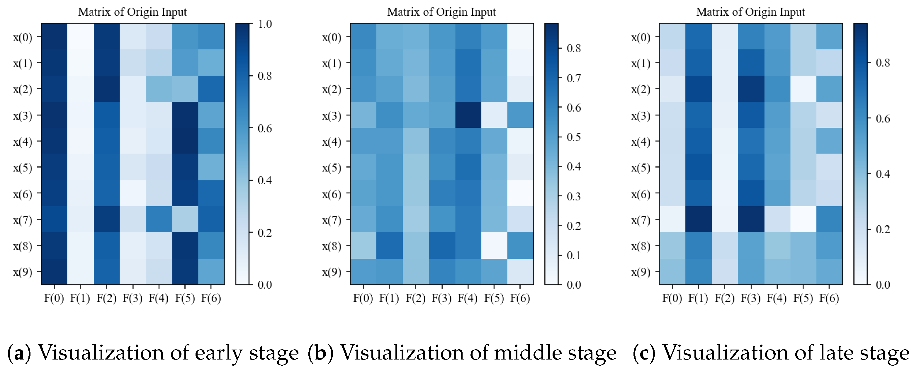
We conducted a self-interpretability analysis of the TLSAM-LSTM framework to elucidate its internal mechanisms. Figure 8 visualizes input data matrices across three battery aging stages: (a) early-stage (first aging cycle), (b) mid-stage (50% EOL cycles), and (c) late-stage (80% EOL cycles). In these visualizations, the Y-axis represents sliding time-window instances ( x ( i ) ) while the X-axis denotes sensor-derived features ( F ( i ) ), with color intensity indicating degradation severity. Although spatial data points exhibit discernible patterns, their relative importance remains indeterminate prior to processing.
The self-attention mechanism (SAM) layer addresses this limitation by concentrating model focus on critical features and temporal instances, significantly enhancing LSTM’s convergence toward optimal SOH estimation. Further interpretability analysis is provided in Figure 9, where subfigure (a) visualizes the attention weight matrix W A , and subfigures (b)–(d) display SAM outputs Z ^ 1 for early, mid, and late degradation stages, respectively. Color intensity in these outputs directly correlates with feature/instance significance, revealing two key insights: feature-level importance substantially outweighs temporal instance-level influence, and among the selected features, F ( 2 ) exerts predominant impact on SOH estimation followed by secondary influence from F ( 5 ) , with remaining features serving auxiliary roles.

3.4. Results

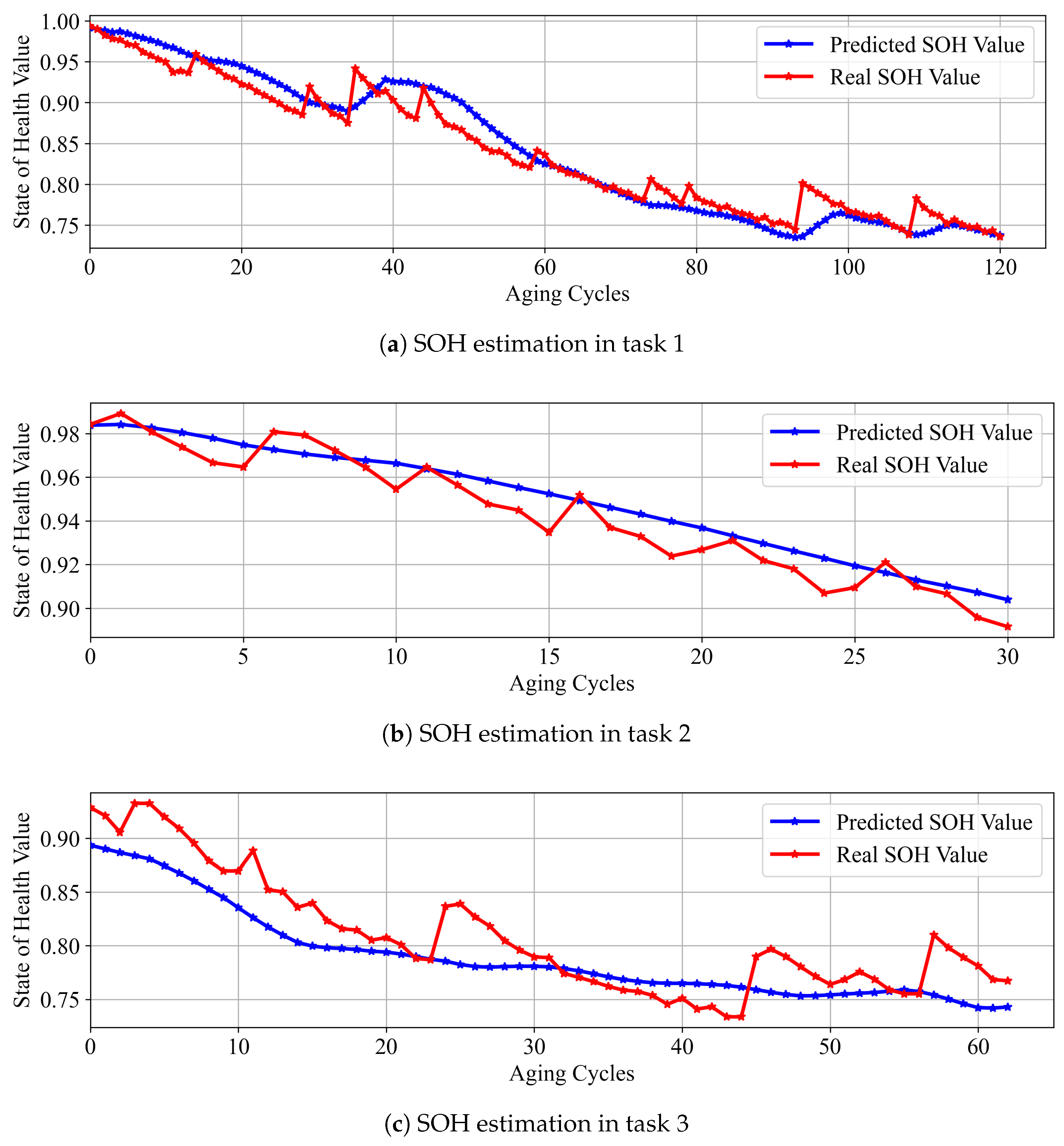
In order to validate the performance of the proposed TLSAM-LSTM method, three tasks are set here. The SOH estimation results of the proposed method under cross-domain conditions are shown in Figure 10. From the results, it can be seen that the TLSAM-LSTM proposed in this paper has accurate prediction effect in all tasks. Meanwhile, twenty repetitive experiments have been conducted under different random seeds. This can explain the effectiveness of algorithms from a statistical perspective. KMM and SAM methods can re-weight the samples from each data point to assign the positive impact on important data. To find the better impact factor of proposed methods, the ablation experiment results have been conducted here as shown in Table 5. From the results, source domain data cannot completely improve the performance of the training model in the target domain. In task 2, due to the difference between source and target domain, direct information transfer will cause large negative impacts. Through the ablation experiment, in task 1 and 3, SAM has better promotion effect than KMM. However, in task 2, the improvement effect of KMM is more obvious, which is the reason for the large difference between source and target domain, and transfer learning has better promotion effect.
After the comparison, some conclusions can be achieved here. First, after training by source, the pre-trained models are easier to estimate accurately after training in the target domain. Then, without any transferred methods, the addition of source data can bring a negative impact into the model training. In addition, KMM can get more obvious improvement when there is a large distribution limitation between source and target. Lastly, it proves that the proposed TLSAM-LSTM can obtain a better performance among all algorithms with a small standard deviation. The couple of SAM and KMM can improve the results robustly and accurately, and the increasing performance is about 30% and 50% on average compared with original algorithms.

Discussion

This study validated the TLSAM-LSTM framework for cross-domain battery SOH estimation using CALCE and NASA datasets, achieving superior performance via dual-weighting mechanisms: KMM mitigates domain shift by re-weighting source samples, while the SAM prioritizes critical aging-related features. In cross-domain tasks, the model achieved the lowest MAPE and RMSE, confirming its robustness for cell-level SOH estimation. Notably, the current work focuses solely on individual cells, while has limitations with practical applications rely on battery packs where the bucket effect dominates [35,36]. Meanwhile, it is important for more data-driven methods to integrate impedance into features engineering. Therefore, future works will extend the framework to pack-level monitoring and detailed feature engineering works.

4. Conclusions

The proposed TLSAM-LSTM model in this paper can achieve better performance on SOH estimation under multiple operating conditions. To verify the results, the CALCE and NASA datasets are employed with data acquisition and preprocessing. ITL can reduce the impact of dissimilar samples, and SAM can achieve the re-weighting calculation of input features, which can have a better interpretability by visualization. The similar source data is used in model training, and can have a positive transfer effect on SOH estimation. Besides, the proposed TLSAM-LSTM model can achieve the better information mining from transferred knowledge. In converter-dominated microgrids, multi-timescale interactions further complicate dynamic behavior and stability assessment, as reviewed in [37]. Through the repeated experiments, the proposed method can have an improvement of about 30% and 50% on average, and have also the best performance between other existing algorithms. At the grid-integration layer, power quality constraints and harmonic mitigation strategies continue to evolve, including metaheuristic approaches based on atomic orbital search and feedback artificial tree control [38].
In the future, we will focus on addressing the time-consuming issue of model training and mitigating negative transfer in such regression scenarios for SOH estimation. We will also integrate impedance-related indicators (e.g., ohmic resistance and charge transfer resistance) into the TLSAM-LSTM framework. We will expand the current input feature set with impedance parameters, leverage the self-attention mechanism to quantify their contribution to SOH estimation, and validate the optimized model with dedicated capacity–impedance paired data, thereby enhancing the comprehensiveness and practicality of the battery health monitoring model.

Author Contributions

Conceptualization, R.H. and J.Z.; methodology, R.H., C.W. and Y.W.; software, R.H., C.W. and C.Y.; validation, R.H., C.W. and C.Y.; formal analysis, R.H., C.W. and C.Y.; investigation, R.H., Y.F. and S.Y.; resources, K.C., Y.F. and S.Y.; data curation, R.H., C.W., C.Y., Y.F. and S.Y.; writing—original draft preparation, R.H.; writing—review and editing, C.W., Y.W., K.C., Y.F. and J.Z.; visualization, R.H., C.W. and S.Y.; supervision, Y.W., K.C. and J.Z.; project administration, Y.W. and J.Z.; funding acquisition, K.C. and J.Z. All authors have read and agreed to the published version of the manuscript.

Funding

This work was supported in part by the National Natural Science Foundation of China under Grant Number 62273074, and 92571201, Sichuan Provincial Science and Technology Support Program under Grant Number 2024NSFJQ0015, the Postdoctoral Fellowship Program and China Postdoctoral Science Foundation under Grant Number BX20250397, China Postdoctoral Science Foundation under Grant Number 2025M771733, the Fundamental Research Funds for the Central Universities under Grant ZYGX2025XJ020.

Data Availability Statement

The original contributions presented in this study are included in the article. Further inquiries can be directed to the corresponding authors.

Conflicts of Interest

The authors declare no conflicts of interest.

References

  1. Yao, L.; Xu, S.; Tang, A.; Zhou, F.; Hou, J.; Xiao, Y.; Fu, Z. A review of lithium-ion battery state of health estimation and prediction methods. World Electr. Veh. J. 2021, 12, 113. [Google Scholar] [CrossRef]
  2. Zhang, J.; Jiang, Y.; Li, X.; Huo, M.; Luo, H.; Yin, S. An adaptive remaining useful life prediction approach for single battery with unlabeled small sample data and parameter uncertainty. Reliab. Eng. Syst. Saf. 2022, 222, 108357. [Google Scholar] [CrossRef]
  3. Ge, M.F.; Liu, Y.; Jiang, X.; Liu, J. A review on state of health estimations and remaining useful life prognostics of lithium-ion batteries. Measurement 2021, 174, 109057. [Google Scholar] [CrossRef]
  4. Belhachat, F.; Larbes, C.; Bennia, R. Recent advances in fault detection techniques for photovoltaic systems: An overview, classification and performance evaluation. Optik 2024, 306, 171797. [Google Scholar] [CrossRef]
  5. Tian, J.; Jiang, Y.; Zhang, J.; Luo, H.; Yin, S. A novel data augmentation approach to fault diagnosis with class-imbalance problem. Reliab. Eng. Syst. Saf. 2024, 243, 109832. [Google Scholar] [CrossRef]
  6. Zhang, J.; Tian, J.; Alcaide, A.M.; Leon, J.I.; Vazquez, S.; Franquelo, L.G.; Luo, H.; Yin, S. Lifetime extension approach based on the Levenberg–Marquardt neural network and power routing of DC–DC converters. IEEE Trans. Power Electron. 2023, 38, 10280–10291. [Google Scholar] [CrossRef]
  7. Xiang, K.; Song, Y.; Ioannou, P.A. Nonlinear Adaptive PID Control for Nonlinear Systems. IEEE Trans. Autom. Control 2025, 70, 7000–7007. [Google Scholar] [CrossRef]
  8. Jiang, Y.; Zhang, J.; Xia, L.; Liu, Y. State of health estimation for lithium-ion battery using empirical degradation and error compensation models. IEEE Access 2020, 8, 123858–123868. [Google Scholar] [CrossRef]
  9. Li, Y.; Wei, Z.; Xie, C.; Vilathgamuwa, D.M. Physics-Based Model Predictive Control for Power Capability Estimation of Lithium-Ion Batteries. IEEE Trans. Ind. Inform. 2023, 19, 10763–10774. [Google Scholar] [CrossRef]
  10. Wang, S.; Gao, H.; Takyi-Aninakwa, P.; Guerrero, J.M.; Fernandez, C.; Huang, Q. Improved Multiple Feature–Electrochemical Thermal Coupling Modeling of Lithium-Ion Batteries at Low-Temperature with Real-Time Coefficient Correction. Prot. Control Mod. Power Syst. 2024, 9, 157–173. [Google Scholar] [CrossRef]
  11. Zhang, H.; Sun, H.; Kang, L.; Zhang, Y.; Wang, L.; Wang, K. Prediction of Health Level of Multiform Li–S Batteries Based on Incremental Capacity Analysis and an Improved LSTM. Prot. Control Mod. Power Syst. 2024, 9, 21–31. [Google Scholar] [CrossRef]
  12. Yang, X.; Chen, Y.; Li, B.; Luo, D. Battery states online estimation based on exponential decay particle swarm optimization and proportional-integral observer with a hybrid battery model. Energy 2020, 191, 116509. [Google Scholar] [CrossRef]
  13. Lin, C.; Xu, J.; Hou, J.; Liang, Y.; Mei, X. Ensemble Method with Heterogeneous Models for Battery State-of-Health Estimation. IEEE Trans. Ind. Inform. 2023, 19, 10160–10169. [Google Scholar] [CrossRef]
  14. Guo, P.; Cheng, Z.; Yang, L. A data-driven remaining capacity estimation approach for lithium-ion batteries based on charging health feature extraction. J. Power Sources 2019, 412, 442–450. [Google Scholar] [CrossRef]
  15. Li, X.; Sun, Y.; Lin, J.; Yin, S. The Synergy of Seeing and Saying: Revolutionary Advances in Multi-modality Medical Vision-Language Large Models. Artif. Intell. Sci. Eng. 2025, 1, 79–97. [Google Scholar] [CrossRef]
  16. Zhang, J.; Qian, K.; Luo, H.; Liu, Y.; Qiao, X.; Xu, X.; Tian, J. Process monitoring for tower pumping units under variable operational conditions: From an integrated multitasking perspective. Control Eng. Pract. 2025, 156, 106229. [Google Scholar] [CrossRef]
  17. Chang, C.; Wang, Q.; Jiang, J.; Wu, T. Lithium-ion battery state of health estimation using the incremental capacity and wavelet neural networks with genetic algorithm. J. Energy Storage 2021, 38, 102570. [Google Scholar] [CrossRef]
  18. Choi, Y.; Ryu, S.; Park, K.; Kim, H. Machine learning-based lithium-ion battery capacity estimation exploiting multi-channel charging profiles. IEEE Access 2019, 7, 75143–75152. [Google Scholar] [CrossRef]
  19. Li, P.; Zhang, Z.; Xiong, Q.; Ding, B.; Hou, J.; Luo, D.; Rong, Y.; Li, S. State-of-health estimation and remaining useful life prediction for the lithium-ion battery based on a variant long short term memory neural network. J. Power Sources 2020, 459, 228069. [Google Scholar] [CrossRef]
  20. Ben-David, S.; Blitzer, J.; Crammer, K.; Kulesza, A.; Pereira, F.; Vaughan, J.W. A theory of learning from different domains. Mach. Learn. 2010, 79, 151–175. [Google Scholar] [CrossRef]
  21. Pan, S.J.; Yang, Q. A survey on transfer learning. IEEE Trans. Knowl. Data Eng. 2009, 22, 1345–1359. [Google Scholar] [CrossRef]
  22. Qian, Q.; Zhang, B.; Li, C.; Mao, Y.; Qin, Y. Federated transfer learning for machinery fault diagnosis: A comprehensive review of technique and application. Mech. Syst. Signal Process. 2025, 223, 111837. [Google Scholar] [CrossRef]
  23. Yu, F.; Xiu, X.; Li, Y. A Survey on Deep Transfer Learning and Beyond. Mathematics 2022, 10, 3619. [Google Scholar] [CrossRef]
  24. Qin, Y.; Yuen, C.; Yin, X.; Huang, B. A Transferable Multi-stage Model with Cycling Discrepancy Learning for Lithium-ion Battery State of Health Estimation. IEEE Trans. Ind. Inform. 2022, 19, 1933–1946. [Google Scholar] [CrossRef]
  25. Li, Y.; Sheng, H.; Cheng, Y.; Stroe, D.I.; Teodorescu, R. State-of-health estimation of lithium-ion batteries based on semi-supervised transfer component analysis. Appl. Energy 2020, 277, 115504. [Google Scholar] [CrossRef]
  26. Ye, Z.; Yu, J. State-of-Health Estimation for Lithium-Ion Batteries Using Domain Adversarial Transfer Learning. IEEE Trans. Power Electron. 2021, 37, 3528–3543. [Google Scholar] [CrossRef]
  27. Deng, Z.; Lin, X.; Cai, J.; Hu, X. Battery health estimation with degradation pattern recognition and transfer learning. J. Power Sources 2022, 525, 231027. [Google Scholar] [CrossRef]
  28. Tan, Z.; Luo, L.; Zhong, J. Knowledge transfer in evolutionary multi-task optimization: A survey. Appl. Soft Comput. 2023, 138, 110182. [Google Scholar] [CrossRef]
  29. Qian, Q.; Wen, Q.; Tang, R.; Qin, Y. DG-Softmax: A new domain generalization intelligent fault diagnosis method for planetary gearboxes. Reliab. Eng. Syst. Saf. 2025, 260, 111057. [Google Scholar] [CrossRef]
  30. Tian, J.; Luo, H.; Wu, S.; Yan, P.; Zhang, J. Source-Free Domain Adaptation for Open-Set Cross-Domain Fault Diagnosis. IEEE Trans. Ind. Inform. 2025. [Google Scholar] [CrossRef]
  31. Zhao, K.; Lin, F.; Liu, X. Comprehensive production index prediction using dual-scale deep learning in mineral processing. arXiv 2024, arXiv:2408.02694. [Google Scholar]
  32. Xing, Y.; Ma, E.; Tsui, K.L.; Pecht, M. An ensemble model for predicting the remaining useful performance of lithium-ion batteries. Microelectron. Reliab. 2013, 53, 811–820. [Google Scholar] [CrossRef]
  33. Saha, B.; Goebel, K. Battery Data Set. NASA Ames Prognostics Data Repository (2007). Available online: http://ti.arc.nasa.gov/project/prognostic-data-repository (accessed on 1 January 2025).
  34. Tan, Y.; Zhao, G. Transfer learning with long short-term memory network for state-of-health prediction of lithium-ion batteries. IEEE Trans. Ind. Electron. 2019, 67, 8723–8731. [Google Scholar] [CrossRef]
  35. Qi, F.; Zhou, Y.; Zhang, Y.; Shen, X.; Hou, E.; Ci, S. Topology Construction Based on Graph Theory for SOC Balancing in Dynamic Reconfigurable Battery System. In Proceedings of the 2025 IEEE International Conference on Electrical Energy Conversion Systems and Control (IEECSC), Chongqing, China, 23–25 May 2025; pp. 615–622. [Google Scholar] [CrossRef]
  36. Li, Q.; Tan, H.; Wang, T.; Wang, S.; Chen, W. Hierarchical and Domain-Partitioned Coordinated Control Method for Large-Scale Fuel Cell/Battery Cluster Hybrid Power Electric Multiple Units. IEEE Trans. Transp. Electrif. 2025. [Google Scholar] [CrossRef]
  37. Zhang, M.; Han, Y.; Liu, Y.; Zalhaf, A.S.; Zhao, E.; Mahmoud, K.; Darwish, M.M.F.; Blaabjerg, F. Multi-Timescale Modeling and Dynamic Stability Analysis for Sustainable Microgrids: State-of-the-Art and Perspectives. Prot. Control Mod. Power Syst. 2024, 9, 1–35. [Google Scholar] [CrossRef]
  38. Kiruthiga, B.; Karthick, R.; Manju, I.; Kondreddi, K. Optimizing harmonic mitigation for smooth integration of renewable energy: A novel approach using atomic orbital search and feedback artificial tree control. Prot. Control Mod. Power Syst. 2024, 9, 160–176. [Google Scholar] [CrossRef]
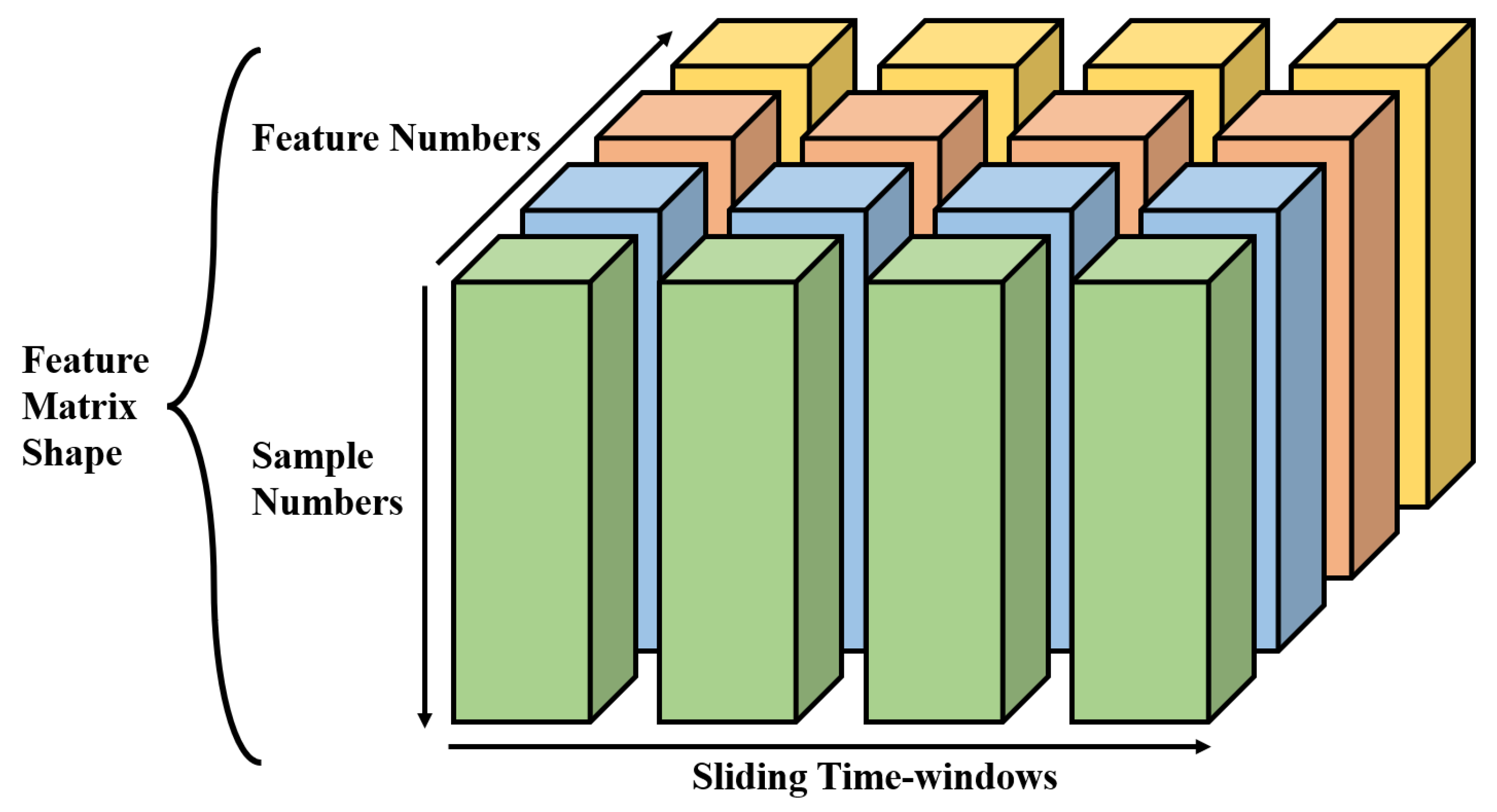
Figure 1. Feature matrix shape of sliding time-windows method.
Energies 18 05672 g001
Figure 2. Detailed framework of TLSAM-LSTM method.
Energies 18 05672 g002
Figure 3. The detailed self-attention mechanism structure.
Energies 18 05672 g003
Figure 4. The detailed long short-term memory structure.
Energies 18 05672 g004
Figure 5. The schematic diagram of SAM-LSTM structure.
Energies 18 05672 g005
Figure 6. State-of-health value in full life aging cycles under four different operating conditions.
Energies 18 05672 g006
Figure 7. Compared results of TLSAM-LSTM model hyper-parameters. (a) RMSE value of learning rate; (b) MAPE value of learning rate; (c) RMSE value of sliding time windows; (d) MAPE value of sliding time windows; (e) RMSE value of layer nodes; (f) MAPE value of layer nodes.
Energies 18 05672 g007
Figure 8. Data matrix visualization of input layers.
Energies 18 05672 g008
Figure 9. Visualization of self-attention layers. (a) Weight matrix visualization of self-attention layers; (b) output visualization of early stage; (c) output visualization of middle stage; (d) output visualization of late stage.
Energies 18 05672 g009
Figure 10. SOH estimation results of the proposed TLSAM-LSTM model.
Energies 18 05672 g010
Table 1. Batteries with operating parameters under different conditions.
InformationDomain 1Domain 2Domain 3Domain 4
Data SourceCALCENASANASANASA
Used DatasetsCS-35∼38B-05/18B-29/32B-45/47
Num of Samples232429762126
I D C (A)1241
V D r o p (V)2.7(2.7/2.5)(2.0/2.7)(2.0/2.5)
T A C-24244
C R (Ahr)1.1222
Other Information L i C o O 2 cathode
prismatic shape
18,650 lithium-ion cells
Table 2. Detailed feature extraction and instrument.
NumFeature Instrument
F 0 Time ratio between CC and CV stage
F 1 Average voltage of early CC stage (Start to 3.85 V)
F 2 Time interval of early CC stage
F 3 Time interval of later CC stage
F 4 Average voltage of later CC stage (3.85 V to end)
F 5 Time interval of CV stage
F 6 Average current of CV stage
Table 3. Detailed task setting situation.
TaskTraining SetTest Set
SourceKnown TargetUnknown Target
Task 1Domain 1,3,4NASA B0005NASA B0018
Task 2Domain 1,2,4NASA B0029NASA B0032
Task 3Domain 1,2,3NASA B0045NASA B0047
Table 4. Hyper-parameters settings of TLSAM-LSTM model.
Hyper-ParametersConfiguration
Feature variables7
Sliding time-windows10
Attention layers7/16
LSTM layers128/64
Learning rate0.01
Epoch (pre-train step)100
Epoch (fine-tuning step)50
Batchsize64
Loss functionMean square error
OptimizerAdam
Table 5. A comparison performance of transfer effectiveness and ablation experiment.
TaskMethodsMAPERMSE
Task 1LSTM-NS4.4888 ± 1.00820.0416 ± 0.0080
CNN-S3.0236 ± 0.28670.0320 ± 0.0031
LSTM-S3.0082 ± 0.57330.0313 ± 0.0051
LSTM-PS2.6763 ± 0.37400.0281 ± 0.0034
TL-LSTM2.6279 ± 0.34040.0278 ± 0.0032
SAM-LSTM1.9826 ± 0.37580.0212 ± 0.0034
TLSAM-LSTM1.8005 ± 0.37190.0198 ± 0.0032
Task 2LSTM-NS1.2248 ± 0.60320.0132 ± 0.0059
CNN-S5.1264 ± 0.35450.0588 ±0.0031
LSTM-S5.9450 ± 1.35160.0613 ± 0.0114
LSTM-PS0.9295 ± 0.14910.0100 ± 0.0016
TL-LSTM0.8990 ± 0.15100.0097 ± 0.0016
SAM-LSTM0.9083 ± 0.24430.0098 ± 0.0023
TLSAM-LSTM0.7944 ± 0.11060.0086 ± 0.0011
Task 3LSTM-NS4.7160 ± 1.26340.0504 ± 0.0169
CNN-S5.2641 ± 0.88410.0498 ± 0.0079
LSTM-S3.7969 ± 0.72570.0358 ± 0.0066
LSTM-PS3.5022 ± 0.83440.0344 ± 0.0074
TL-LSTM3.0893 ± 0.54700.0296 ± 0.0048
SAM-LSTM2.8358 ± 0.60000.0297 ± 0.0056
TLSAM-LSTM2.5917 ± 0.50870.0282 ± 0.0045
Disclaimer/Publisher’s Note: The statements, opinions and data contained in all publications are solely those of the individual author(s) and contributor(s) and not of MDPI and/or the editor(s). MDPI and/or the editor(s) disclaim responsibility for any injury to people or property resulting from any ideas, methods, instructions or products referred to in the content.