Abstract
The economic benefit of a 12.8 kWp photovoltaic (PV) system was calculated using real consumption and electricity generation data for a typical modern single-family house in Sweden for the six years between 2019 and 2024. Electricity trade prices were based on the local spot market plus taxes and fees. The effect of a tax reduction on exported electrical energy was evaluated. The economic benefit was simulated for the case of a virtual AC-coupled battery added to the house using a charging strategy to maximize the self-consumption of the house. Additionally, the economic benefit was simulated for a range of different yearly consumptions and PV system sizes. The calculation shows that the PV system alone can be economically beneficial, while adding a battery with typical investment prices from 2025 does not pay off if it is only used to increase the self-consumption rate.
Keywords:
photovoltaics; economics; solar cell system; battery; simulation; energy storage; Sweden; electricity costs 1. Introduction
Sweden aims to reach zero greenhouse gas emissions by 2045 [1]. Photovoltaics (PV) will play a significant role in reaching this target, provided that sufficient incentives exist to install them. Because electricity is consumed mainly in cities, it makes sense to use the roofs of buildings in urban areas for PV systems to minimize the distance between consumers and prosumers and increase supply security through decentralized electricity generation sites. With only 3.7% theoretical PV penetration by the end of 2024, Sweden is behind most other European countries in using this valuable and cheap energy source [2]. This might be surprising, because the yearly sun irradiation in the most populated part (southern Sweden) is only slightly less than that in Germany (with nearly 20% PV penetration) [3]. One reason might be that Swedish buildings use more electrical heating systems which in turn entails a strong demand during the winter months with low sun irradiation. Furthermore, electricity prices are significantly lower in Sweden than in Germany, making it less economically beneficial to generate electricity with PV [4]. An overview of solar PV subsidies in Sweden between the years 2009 and 2021 is given by Rydehell et al. [5], analyzing the relationship between policy incentives and subsidy applications for different types of investors. One question behind the research presented here is if it would be economically beneficial to invest in a battery energy storage system (BESS) to increase the amount of self-consumed electricity from a PV system. A questionnaire among Swedish farmers who already own a PV system about their willingness to invest in a BESS revealed that reducing costs is a major driver, although the risk of poor battery performance and uncertainty about the investment aid present major barriers for such an investment [6].
It can generally be assumed that the economic benefit is the major driver for house owners to install PV systems [7,8]. The decision to invest in PV with or without BESS often lies with the house owner and typically depends on whether the investment will pay off within a reasonable time period. To answer this question, detailed information on the expected financial savings from the system is required. Machine learning models can predict the self-consumption rate (as defined in Equation (1) below) based on annual electrical load, annual PV electricity generation, and tilt angle and azimuth angle of the modules and the latitude [9,10,11]. Such models, when provided via a suitable application, can help house owners with their decision. Several online calculators are available for the economic payback time, but they unfortunately give a large range of different results, like 7 to 18 years for the same house, as demonstrated by Sommerfeldt et al. [12].
Zainali et al. calculated the average levelized cost of PV electricity (LCOE) based on a statistical evaluation of over 6000 single-family dwellings in Sweden during 2019 and 2020. The mean value of the unsubsidized LCOE was about SEK 1/kWh when assuming a real discount rate of 2% for the investment [13]. This price must be compared to the actual electricity tariffs to estimate the economic benefit over time. However, this becomes a challenging task when tariffs change hourly or even include power-based tariffs.
Power-based tariffs, called “capacity charges” or “demand charges”, depend on the largest power peak or an average of the largest power peaks during a certain period, for example a month. These prices can vary across seasons, and reducing factors can be added to the measured power during certain hours, for instance during the night.
With rising amounts of PV and wind power, strategies must be developed to balance an increasingly volatile energy supply [14]. In 2022, the Swedish Energy Markets Inspectorate (Energimarknadsinspektionen) decided that capacity charges must be included in the electricity tariffs for end users from January 2027 at the latest [15]. The aim was to foster a more efficient use of the electricity grid by adding an incentive to avoid high power peaks. On the other hand, many Swedish households already have time-varying electricity tariffs, which already is an incentive to reduce electricity consumption during periods of high demand when the prices are higher. Based on a study by Lundgren et al., the authors concluded that the introduction of time-varying distribution tariffs did not affect the efficiency of the grids [16]. Little evidence of power tariffs influencing consumption behavior was found [17]. As shown later in this paper, Swedish electricity tariffs in 2025 can comprise over 20 different parameters, several of them varying over time. This makes it challenging for house owners to understand how to reduce their energy costs.
A battery storage system can be used to increase the self-consumption or the self-sufficiency rate, which are defined as
A few studies on the economic benefits of PV systems, partly including battery energy storage systems, have been conducted using real Swedish electricity tariffs. Fiedler et al. have analyzed the economy of PV and BESS using consumption data from four grid-connected holiday houses in Sälen, Sweden [18]. The benefits of virtual PV systems and batteries were simulated based on three different electricity tariffs. The authors concluded that BESSs are highly profitable in environments where distribution system operators (owners of the grid connecting the house) invoice capacity charges that depend on the highest consumption peaks of the month. The calculations were based on a simulated advanced battery control strategy, including forecasting peak loads and electricity prices to implement peak shaving and increase self-consumption. However, these strategies might not be fully available in today’s existing battery controllers. Profitability also strongly depends on governmental subsidies for these systems.
Ruan et al. evaluated the technical and economic potential of using roofs in Hammarby Sjöstad, which is a district of Stockholm, assuming two virtual scenarios of PV system expansions [19]. Dividing this district into 19 sub-areas, the self-consumption and self-sufficiency rates per sub-area were calculated for both scenarios. In the scenario with the largest expansion of PV, self-sufficiency rates mainly between about 5% and about 20% were reached, while the self-consumption was over 90% in most cases. The calculated net present values of the analyzed PV systems ranged from positive to negative, strongly depending on assumed electricity prices and financial support from the government. This means that the investments in the modeled PV systems (even without batteries) would potentially not pay off during their lifetimes.
Ollas et al. have analyzed the impact of a simulated BESS on a nearly zero energy single family house in southern Sweden which had a 7.2 kWh PV system, using real and partly simulated consumption data of about one year [20]. Three different dispatch algorithms for the virtual battery were simulated. One algorithm was used to maximize the self-consumption rate (as defined above in Equation (1)). Two other algorithms were applied for peak shaving of the power imported from the grid, one of them using a perfect prognosis of electricity generation and consumption data from the day ahead, the other one assuming that this data is equal to the day before. The study mainly calculates the average peak-power values and the self-consumption rates for these three algorithms, but does not take real electricity tariffs into account. The authors of this 2018 study conclude that the investment in a BESS might in many cases not be justified.
Luthander simulated the effect of virtual PV systems and batteries from 21 detached single-family houses in Sweden [21] using a kinetic lead-acid battery model by Manwell and McGowan [22]. Real consumption data was used, collected by the Swedish Energy Agency during a monitoring campaign between 2005 and 2008 [23]. PV system sizes between 2.2 and 11 kW were simulated based on the real orientation and areas of the roofs. The virtual batteries were simulated to be charged only with surplus electricity from the PV systems and discharged when the consumption exceeded the electricity generation from the PV systems. The study mainly reports the effect of BESS sizes on the self-consumption rate for separate and combined electricity meters, as well as the effect of curtailment of power fed to the grid for the overall power loss. Assuming fixed electricity prices, the relative changes in economic revenues were calculated for different scenarios. The authors conclude that sharing BESS and electricity meters in a community of end-users increases the economic revenues compared with not sharing.
Having a PV system with a fixed size, the self-consumption rate can generally be increased using BESS or demand side management (DSM). The latter is a concept to shift the electric load in a household towards hours with surplus PV electricity generation [24,25]. DSM can be done manually, for example with dish washers, washing machines, or electrical heating systems. To some extent, manual DSM might be applied by house dwellers, if they clearly benefit from this. A study from 2018, however, shows no clear trend in behavior after PV installation [26]. The limiting factors can, for example, be working times or school hours. Automatic DSM, however, requires a control unit connected to appliances with suitable interfaces and protocols, which is still challenging to set up today.
The novelty of the work of this paper is in analyzing real measured data of consumed electricity and generated photovoltaic electricity in combination with real variable electricity prices and variable size factors for the PV system, house consumption, and a virtual battery.
In this work, a strategy to maximize the self-consumed PV energy using a virtual BESS is investigated based on actual hourly based consumption and PV electricity generation data.
2. Methods
2.1. The Test House
The data evaluated here were obtained from a typical modern Swedish single-family house in Värmland with a 131 m2 heated area, built in 2018. For six years between 2019 and 2024, the imported and exported energy (The term “energy” means “electrical energy” throughout this article) for the house was collected on an hourly basis, as measured by the smart meter provided by the distribution system operator. The house is equipped with a photovoltaic (PV) system with 45 modules based on multicrystalline silicon solar cells (Q-cells, Selangor, Malaysia, Q.PLUS BFR-G4.1 285) with a nominal 12.8 kW DC peak power. The roof has a 34-degree inclination towards the horizon and is oriented in a southwest direction (202° azimuth counted from the north). The PV system comprises a 10 kW inverter (SMA, Niestetal, Germany, Sunny Tripower 10000TL), which was chosen to keep the generated current per line below the three-phase house fuses of 16 A and therefore obtain the lowest possible base tariff from the distribution system operator.
The PV electricity generation data were regularly downloaded from the inverter at 5 min time intervals. During a few periods, only 15 min time intervals could be obtained. In rare cases, missing PV electricity generation data were reproduced (see Appendix A). All sub-hourly data were summed up to full-hour time intervals.
On average, the yearly PV electricity generation was 12,635 kWh, and the energy consumption of the house was 7468 kWh. Most of the consumption (approximately 4500 kWh) was used for heating by an exhaust-air heat pump (Nibe, Markaryd, Sweden, F730) connected to floor heating. On some cold days, the house received additional heat from a fireplace. The average self-consumption rate of PV energy was 16.8%, corresponding to 2123 kWh annually. Therefore, the actual yearly imported energy was 5345 kWh. Compared to older Swedish houses with less effective thermal isolation and older heating systems, this consumption is slightly lower. It therefore represents rather the housing standards of the coming years.
The price of the PV system was SEK 160,000 minus a subsidy of 30% (SEK 48,000) from the state of Sweden.
2.2. The Prices for Electrical Energy
Swedish households recently reached 100% smart meter penetration, enabling all household dwellers to use dynamic electricity tariffs [27,28]. The Swedish electricity prices can be quite complicated, comprising about 23 different parameters, which are listed in Appendix B. The household owner typically has one contract with the electricity supplier and another one with the distribution system operator. Some price parameters (for example the spot prices) vary every hour, others every month, or in longer intervals. Sweden is subdivided into four geographical electricity price regions SE1–SE4, with S1 comprising the northern territories and SE4 the south. Each electricity region has its own hourly spot market prices. SE1 typically has the lowest prices due to large electricity generation by hydropower in the region and lower population density.
Additionally, capacity charges (effektavgifter) can be added depending on the consumption power peaks of the month. For this type of charge, the average imported power during each hour is used. Between 22 h and 6 h every day, this power is multiplied by a factor of 0.5 in the calculations, which use a power tariff (see Table 1 below). The resulting power values are sorted at the end of each month, and the three largest values are averaged. This average value is multiplied by the capacity charge per kW and charged at the end of the month.

Table 1.
Parameters of the electricity tariff. The quantities are explained in detail in the text above.
If no constant prices per kWh are contracted, the prices for trade with the electricity supplier include hourly based spot prices provided by the Nordpool group [29]. These prices are announced for the day ahead around noon. When purchasing electrical energy, a value-added tax (VAT) of 25% is added to the spot price. Selling surplus electrical energy from the PV electricity generation can also include spot prices, but without VAT. Every purchased kWh is additionally charged with an energy tax by the Swedish state. This tax is invoiced by the distribution system operator. The Table A2 in Appendix B gives an example of the electricity price parameters.
For the simulations presented here, some parameters are merged, and the formulas (3)–(5) were used with the averaged values given below (for instance, Itrade is a sum of parts 3–9 in Table A2 in the Appendix B). The costs from the distribution system operator were calculated with or without power tariffs as described in the text (from 2019 until 2024, the value of Igrid was significantly larger (around SEK 0.3/kWh) and Igrid power price was zero. The capacity charge was first introduced by the distribution system operator from 2025. Because this publication should be used for future applications, it was decided to use the price tariffs including power price as given directly below (Equations (3)–(5)). Fixed monthly costs were not taken into account, because they are the same for all compared scenarios.
with Itrade: import price per kWh from the electricity supplier, S: Nordpool’s spot price per kWh (changing every hour), Itax: electricity tax per imported kWh, Igrid: transfer fee per imported kWh from the distribution system operator, I0: imported energy, Etrade: export price per kWh paid by the electricity supplier, Egrid: export price per kWh paid by the distribution system operator, E0: exported energy, Igrid capacity charge: capacity charge per W by the distribution system operator, Pavg: average power over the three largest weighted power peaks as described above, and Elimit: yearly exported energy, limited to the amount of imported energy. The parameters of the electricity tariff are listed in Table 1. In Tariff B, the value of Igrid capacity charge is multiplied by a factor of 0.5 during night hours from 22 h to 6 h. The values of the quantities correspond to certain part numbers of Table A2 in the Appendix B. These numbers are given in brackets in the following. I-symbols represent imported energy and E-symbols represent exported energy. The value of Itrade was calculated as an average of the sum of tariffs (parts 3 to 9) for the year 2024. Itax is the energy tax from the Swedish state (part 2) for 2024. The value of Igrid is the transfer fee from the distribution system operator for imported energy (14). The value of Etrade was calculated as an average over the months from April 2024, where it was first introduced, to December 2024 (part 12). The export price per kWh Egrid was used from low grid load periods (22). Igrid capacity charge is the price calculated for the average of the three largest power peaks of the month as described above (16). Etax reduction was a tax reduction by the Swedish state that paid for exported energy up to the amount of kWh that was imported during that year. This tax reduction will be removed as of 1 January 2026. The calculations presented here use the spot price values of region SE3. Negative costs denote an income for the prosumer.
Instead of tariff part number 22 in Table A2, part number 21 was used the whole year, because low exported energy occurs from November until March, making the difference negligible.
2.3. Simulation of an Optional Battery
The economic benefit of a PV system increases with increased self-consumption, because self-generated energy is not subject to taxation or grid-related charges. It was therefore calculated to what extent a battery energy storage system (BESS) would have increased the economic benefit. The calculated benefit presented here does not include investment costs for the BESS. In the following, the term “return” will be used to denote the economic benefit from savings and remuneration by selling electricity.
Based on the measured hourly imported, generated, and exported energy, the effect of a virtual battery connected to the AC side of the house was simulated using the exact hourly data of consumption, electricity generation, and tariffs. The efficiency for charging and discharging of the battery depends on the ratio of power to the maximum power at the time of charging or discharging [30,31,32,33,34]. The dependency of the efficiency on the charging state is neglected here. For the present calculations, the charging and discharging efficiency curves for the BESS D from Munzke et al. are used [30].
An analysis of the shape of these curves shows that they can be fitted using the empirical formula
where is the charging or discharging efficiency, x is the ratio of maximum power, and a, b, c, d, and e are fit parameters. Because the data from Munzke does not comprise the x-range from 0 to about 5%, this part was extrapolated, constraining the value at x = 0 to = 0.5. The values of the corresponding fit parameters were determined in the work presented here using the data analysis software Origin (version 9.0.0) and are given in Table 2. The efficiency curves are depicted in Figure 1.
Table 2.
Fit parameters for the charging and discharging efficiency curves for the battery storage system using the above equation.
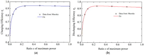
Figure 1.
Charging (a) and discharging (b) efficiency of the AC-coupled battery storage system used in this paper, with fitted curves based on data from the BESS D from Munzke et al. [30].
The assumed strategy for charging and discharging was to maximize self-consumption of the PV system. (The strategy is chosen for simplicity. More complicated strategies for increasing the economic benefit involving forecasts of consumption, etc., are discussed at the end of this paper and could be part of future research). The algorithm for charging and discharging simulation is sketched in Figure 2. The calculation is done for every time interval Δt (1 h). During a single interval, both charging and discharging can occur. Here, the calculation shown in Figure 2a is performed first, followed by the calculation shown in Figure 2b. The quantities used are defined as follows:
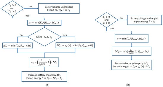
Figure 2.
Charging (a) and discharging (b) calculation flow for the simulated battery storage system to maximize self-consumption of PV energy. The goal is to store surplus energy from the PV system in the battery instead of exporting it, as well as discharge the battery instead of importing energy, if possible.
- C: battery charge;
- ΔCc: increase in battery charge during Δt;
- ΔCd: decrease in battery charge during Δt;
- Cf: free battery capacity (=capacity-charge);
- I0: imported electrical energy without battery (measured);
- E0: exported electrical energy without battery (measured);
- I: virtually imported electrical energy with a battery;
- E: virtually exported electrical energy with battery;
- Pmax: maximum battery power;
- x: used ratio of maximum battery power;
- ηc: charging efficiency function;
- ηd: discharging efficiency function;
- Lc: electrical energy loss during charging.
The algorithm in Figure 2a simulates the charging of the virtual battery during a time step Δt, which was one hour in these calculations. In cases where there is surplus energy from the PV system (E0 > 0) and free battery capacity (Cf > 0), the battery will be charged. The ratio x of maximum battery power is calculated, limited to 1, and is used to calculate the battery charging efficiency ηc(x). The storable amount of energy is ηc(x)·E0, provided that enough free capacity is available. The left path is the case of more energy available than can be stored and makes sure that the battery charge can reach 100%. The right path already uses the fact that some of the available surplus energy is lost due to the imperfect charging efficiency. In both cases the energy transferred into the BESS is limited by the maximum charging power of the battery. ΔCc denotes the amount of energy that ends up in the battery after losses. An energy Lc is lost due to imperfect charging efficiency of the battery. In the end, only the energy E can be exported.
The algorithm in Figure 2b simulates the discharging of the battery during a time step Δt. This algorithm is activated when the house without battery would import energy (I0 > 0) and the battery has some charge C. The ratio x of maximum battery power is calculated, limited to 1, and is used to calculate the battery discharging efficiency ηd(x). In the easiest case, the battery loses some energy ΔCd = I0/ηd(x) which is larger than the needed energy I0 due to its imperfect efficiency. This energy is then limited to the available charge C and by the maximum power of the battery. In the end, the imported energy is reduced by ηd(x)·ΔCd.
An example of the work of this algorithm for a virtual battery with 10 kWh capacity and 10 kW maximum power is presented in Figure 3. The algorithm was applied to the measured data and shows the first week of April 2024. On sunny days, the battery is quickly charged during a few morning hours and discharged during the nights.
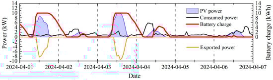
Figure 3.
Calculated battery charge (thick red curve) from the first week of April 2024 using a virtual battery with 10 kWh capacity and 10 kW maximum power. The calculation was done by the algorithm explained above. The black curve shows the real consumed power by the house (self-consumed power + imported power). The blue curve corresponds to the power generated by the PV system. The negative part of the diagram shows the virtually exported power in cases of such a battery.
2.4. Simulation of Different Consumptions
To also cover different consumption scenarios in this investigation, the house consumption was virtually multiplied by a consumption factor fc to simulate houses with larger or smaller yearly electricity consumption. For this, the measured imported energy was replaced by I′ and the measured exported energy was replaced by E′ according to Equations (10) and (11) below, where is the photovoltaic energy generated.
From conservation of energy, we get
where is the consumed energy for the original case with no consumption factor. If the consumption is now changed by the factor fc, we get
Inserting Equation (7) into Equation (8), we get
We have only one Equation (9) for the two unknown quantities and , which means that the problem is underdetermined. Here, we make the assumption
Inserting Equation (10) into Equation (9) we get
It has to be mentioned that for and , we never reach the case of , which might not be realistic in cases for sufficient PV electricity generation. Another variant would be to set if and if and calculate the other unknown quantity using Equation (8). In such a variant, the normal case of would not be correctly calculated if (hours with both import and export). Because we mainly investigate the cases where here, Equations (10) and (11) are used in the following.
These modified values for the imported and exported energy were applied for every hour during the six years of investigation. A factor of was used in this paper if not otherwise stated.
2.5. Simulation of Different Electricity Generations
It is also interesting to think about what economic benefit a smaller or larger PV system would have had. For this virtual case, an electricity generation factor fp was introduced. The virtual generated energy during a time interval is then
It is furthermore assumed that the house consumption is constant at its value
If we name the imported energy and the exported energy for the case of virtually changed electricity generation by a factor , it follows that
The imported energy I′ and the exported energy E′ have to be changed now, because less PV electricity generation would probably reduce the exported energy according to the goal of maximizing self-consumption. If the PV electricity generation was larger, the imported energy would be less. Knowing and , Equation (14) only tells us the difference between I″ and E″, but not their exact values, because we only have one equation for two unknown variables I″ and E″.
As an approximation, one can assume that the exported energy is zero when the PV system delivers less energy than consumed. Also, one can assume that the imported energy is zero when the PV system delivers more energy than is consumed. In both cases, Equation (14) will be used to calculate the other unknown variable.
For , the imported and exported electrical energies are approximated by
For , the imported and exported electrical energies are approximated by
This approximation does not take into account time periods (of one hour) where the measured imported energy and the measured exported energy both are larger than zero. The approximation implicitly increases the calculated benefit a little, because an optimal case is forced for each hour, where, for instance, the imported energy is minimized, although there were some minutes during that hour when the electricity generation was too low. However, this only happens rarely. In the case of Section 3.2.3, this leads to a deviation of the total return of only 0.9% compared to not applying this correction.
3. Results
3.1. Time Series
3.1.1. Photovoltaic Electricity Generation
Figure 4 shows a power curve from the PV system during a sunny day in May 2024. Because the inverter has a maximum power of 10 kW, the power is limited to that value during noon. Such curtailing of power happens only on a few days per year and lowers the yearly PV yield marginally.
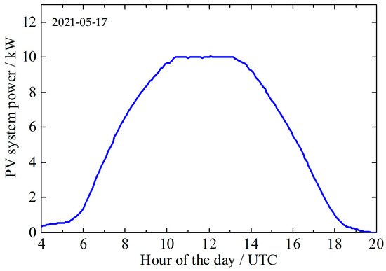
Figure 4.
Power from the PV system during a sunny day in May 2024 as measured by the inverter. The AC-power is limited to 10 kW by the inverter, which happens during a few colder days of the year with a perfectly clear sky.
3.1.2. Self-Consumption of the PV Power
The electricity consumption of the house is the sum of the imported electric energy and the self-consumed electric energy.
Here, is the self-consumed electric energy, E0 the exported electric energy, C0 the consumed electric energy, and I0 the imported electric energy. The hourly averaged values for the PV power, together with the self-consumption and the amount of imported power during a few days in April 2024, are depicted in Figure 5. During sunny days, only a smaller fraction of the PV power is directly self-consumed. When the PV power exceeds the consumption of the house, the surplus power is exported, suppressing the imported power to zero.
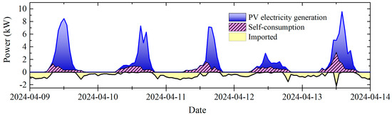
Figure 5.
Hourly averaged power from the PV system with the self-consumption part and imported electricity during a few days in April 2024. The area between the curves for self-consumption and imported electric power corresponds to the consumed electric energy of the house. The blue area between the curves of electricity generation and self-consumption corresponds to the exported electric energy.
Because hourly averaged data are presented here, it can happen that energy is exported and imported during the same hour, but not at the same time. Imported power occurs for instance during short periods in an hour when the sun is shaded by clouds. An example is the little peak of the imported power during noon on the last day in Figure 5.
3.2. Economic Benefit of the PV System Alone
3.2.1. Economic Benefit of the PV System for the Real Case
The first question to be answered was whether the PV system itself was economically beneficial. For that case, the virtual situation of not having a PV system or a battery at all is calculated for each hour. The virtual situation of not having a PV system means that
Here, and are the imported and exported electric energies for the virtual case of not having a PV system or BESS, respectively. For every hour, the electricity costs are calculated for the case of not having a PV system or a battery, and then the costs for the case of having the PV system but no battery are subtracted. This return for every hour is accumulated over the six years. The investment costs of SEK 112,000 for the PV system are not yet included in this calculation.
Without a PV system, the yearly consumption-dependent costs for electricity would have been SEK 15,669 when using the constant tariff B, where about 25% of it corresponds to the capacity charge. “consumption-dependent costs” denote costs excluding fixed monthly costs for having a contract with the electricity retailer and the distribution system operator.
Although the electricity tariffs for the investigated house varied, partly due to changes in the electricity retailer, the constant electricity tariffs from Table 1 are assumed in the following. Figure 6 shows how the yearly consumption costs are reduced by having a PV system without a battery for both tariffs A and B. In both cases, an additional yearly benefit of SEK 3207 would be calculated if the Swedish feed-in premium of SEK 0.60 per exported kWh (applied as an annual tax reduction) up to the amount of imported energy is taken into account. This additional benefit is limited to an amount of 5345 kWh of yearly imported energy. Because this feed-in premium is planned to be removed by the Swedish government from 2026 [35], it will not be used in most of the following sections.
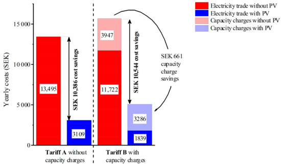
Figure 6.
Yearly electricity consumption costs (without monthly fixed costs) for the electricity tariffs listed in Table 1. No tax reduction of SEK 0.60 per exported kWh is included in both cases. Capacity charges correspond to Igrid capacity charge and electricity trade to all other parts, except Etax reduction. The difference is the total yearly return from the PV system. No battery was assumed.
The yearly total return of the PV system is SEK 10 386 for tariff A and SEK 10,544 for tariff B. The change from tariff A to tariff B increases the yearly costs by SEK 2174 without PV and by SEK 2016 with the PV system. The capacity charges are only reduced by SEK 661 yearly due to the PV system.
Using tariff B, one can calculate the amortization times of the PV system alone, assuming that the total return of SEK 10,544 is used for amortization each year. These times are depicted in Figure 7 depending on different bank interest rates.
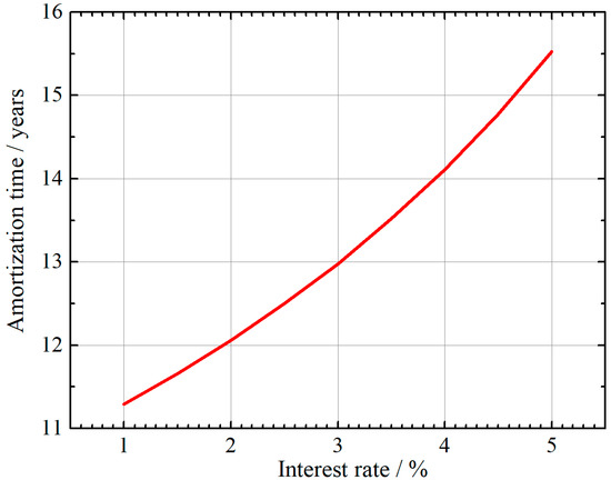
Figure 7.
Amortization time of the PV system alone assuming a purchase price of SEK 112,000 and a total yearly return of SEK 10,544.
3.2.2. Economic Benefit of the PV System for Different Consumption Levels
As mentioned in Section 2.1, the real consumption of the test house is slightly on the lower side. To cover different consumption scenarios, the virtual case of different consumption levels was analyzed using a consumption factor fc, according to Equations (10) and (11). The resulting benefit of the PV system is presented in Figure 8 for the case with capacity charge as described in Section 2.2, no tax reduction subsidies, and no battery.
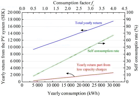
Figure 8.
Dependency of the total yearly return from the PV system for different virtual house consumption values. Also shown is the yearly return from the reduced capacity charge alone and the self-consumption rate. No tax-reduction subsidy is assumed.
3.2.3. Economic Benefit for Virtually Smaller or Larger PV Systems
Using the equations from Section 2.5, the effect of a different PV size is calculated. It is assumed that the PV electricity generation is now changed virtually by an electricity generation factor fp.
Figure 9 shows the result of this calculation for electricity generation factors between 0 and 4. The horizontal scale on the bottom is calculated under the assumption that the PV electricity generation is proportional to the nominal PV system size. The graph shows that the total yearly return almost linearly increases with the PV system size. Only a minor fraction of this return is due to savings in the capacity charge. A self-consumption rate of 50% would be reached for a nominal PV system size of 2.75 kWp.
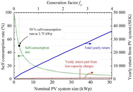
Figure 9.
Total yearly return and self-consumption rate, if the PV electricity generation is virtually changed by an electricity generation factor fp. Also plotted is the part of the yearly return by saving the capacity charge due to the PV system. The vertical line marks the situation of a 50% self-consumption rate. No tax-reduction subsidy is assumed.
3.3. Economic Benefit of a Battery
3.3.1. Economic Benefit of a Battery with Capacity Charge and Tax Reduction Subsidy
This simulation assumes the above-stated capacity charge, which has to be paid at the end of each month, and a tax reduction subsidy of SEK 0.60 for each exported kWh up to the amount of imported energy, which is paid back at the end of each year. The calculation was done for battery sizes between 0 kWh and 10 kWh. The maximum power of the battery in kW was assumed to correspond to the battery capacity in kWh.
Figure 10 shows an expected increase in the total return with increasing battery size. A remarkable result is that this return approaches a maximum and reduces again for battery sizes larger than 2 kWh. It even becomes negative above capacities of 8 kWh. The reason for this decline in return with larger battery capacities is due to a loss of tax reductions, as can be seen in Figure 11. If more energy is self-consumed instead of exported, less tax reduction is paid back to the house owner.
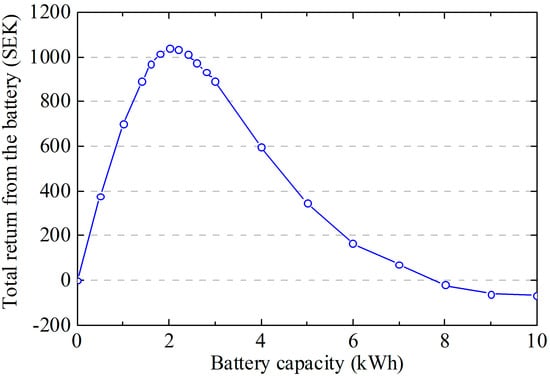
Figure 10.
Total return in SEK for adding a virtual battery to the house for the case of a yearly tax reduction of SEK 0.60 per exported kWh up to the amount of imported electricity. The maximum power of the battery in kW was assumed to correspond to the battery capacity in kWh. The battery can even have a negative impact on the economy for larger capacities. The values correspond to the difference between the return of PV with a battery and the return of PV alone. The line is a linear interpolation of the calculated data points.
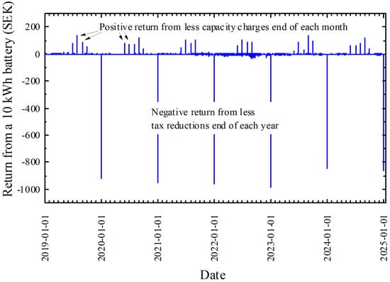
Figure 11.
Difference in return for a 10 kWh battery with 10 kW maximum power and the return for the case of no battery, plotted over the 6 years. The strong negative peaks are due to reduced tax reductions at the end of the year, because less energy is exported with a large battery. The positive peaks at the end of each month correspond to the benefit of lower capacity charges, because less power is consumed during the summer months. The return from less imported energy is not resolved in the graph because it is plotted per hour and therefore has values of the order of one or a few SEK.
3.3.2. Economic Benefit of a Battery with Capacity Charge and No Tax Reduction Subsidy
If the tax reduction in SEK 0.60 per exported kWh is removed, the total yearly benefit of the PV system without a battery is reduced by about SEK 3200. Figure 12 indicates the yearly economic benefit of the PV system with a virtually added battery. Even a 14 kWh battery would only give SEK 1000 of extra benefit per year compared to the PV system without a battery. Because the consumption of the investigated house is on the lower side, the same calculation was done for a house with a virtually doubled consumption as described in Section 2.4. The result is shown in Figure 13. In that situation, the self-consumption rate is significantly increased, and also the total yearly return is increased by SEK 2300–2700 compared to the case with the real consumption. Even with a PV system already installed, the pure part from a 14 kWh battery is still only about SEK 1300 yearly.
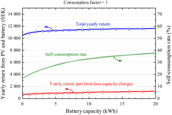
Figure 12.
Simulated yearly return and self-consumption rate from the PV system and battery, assuming tariff B from Table 1, without a yearly tax reduction of SEK 0.60 per kWh exported energy. The maximum power of the battery in kW was assumed to correspond to the battery capacity in kWh. Upper curve: Total yearly return. Lower curve: Share of this yearly return coming from the reduced capacity charge. The lines are a linear interpolation of the calculated data points.
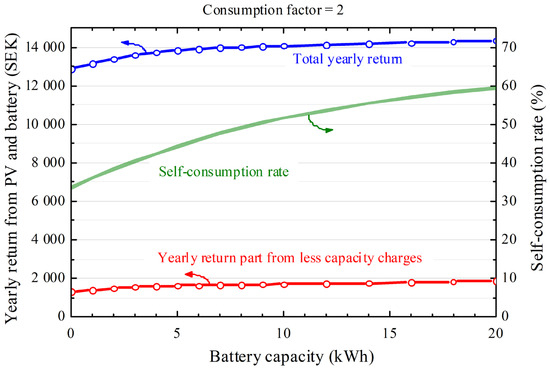
Figure 13.
Simulated yearly return and self-consumption rate from the PV system and battery, assuming tariff B from Table 1, without a yearly tax reduction in SEK 0.60 per kWh exported energy. The house consumption is virtually doubled (fc = 2). The maximum power of the battery in kW was assumed to correspond to the battery capacity in kWh. Upper curve: Total yearly return. Lower curve: Share of this yearly return coming from the reduced capacity charge. The lines are a linear interpolation of the calculated data points.
An interesting effect of the maximum power of the battery is depicted in Figure 14, where only the maximum power of the battery is modified while holding its capacity constant. The economic benefit then has a maximum at around 2 kW. The left side of this graph reveals the fact that the battery cannot be fully used if the power is limited by the maximum power. The curve declines after the maximum because of a lower battery efficiency during increasing time fractions, where the power needed is only a smaller fraction of the maximum power (see the charging and discharging curves in the Methods Section).
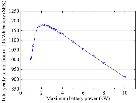
Figure 14.
Simulated total yearly return from a 10 kWh battery added to the house with PV, assuming tariff B with capacity charges, but no yearly tax reduction. The maximum battery power is varied. The line is a linear interpolation of the calculated data points.
4. Discussion and Conclusions
The most important factor in the decision to invest in a PV system and possibly add a battery energy storage system (BESS) is whether it is economically viable. The test case evaluated here should give house owners some help with this decision. Furthermore, it can assist policymakers in estimating the impact of subsidy changes on future market development. The data used represent only a single house and are therefore not statistically significant. However, the electricity generation and consumption factors included in the simulations allow for estimation of the economics of a wider range of houses.
As stated by Munzke et al., many publications presently only include battery efficiencies in a simplified way, for example by assuming only constant values independent of the power used [30]. Because many batteries have maximum power values corresponding to their capacity (e.g., 10 kW for a 10 kWh battery), the reduced charging and discharging efficiencies can play a certain role when the power ranges between 0 and 10% of the maximum value. Such low power values can occur quite often, for instance when discharging the batteries during the night or charging them on cloudy days. Assuming the efficiency curves used here, this suggests not to oversize the maximum battery power.
The PV system alone mainly reduces costs from the electricity retailer and electricity taxes. Only a small part of the benefit is due to the reduced capacity charge if such tariffs are applied. The economic benefit linearly increases with consumption starting from a fixed offset. This offset is due to the selling of energy. Furthermore, the economic benefit was simulated to be nearly proportional to the PV system size.
Tax reductions of SEK 0.60 per exported kWh in Sweden led to a declining economic benefit of BESS with increasing battery capacities. This might be the reason for the government’s decision to remove this tax reduction from 2026 to make batteries more attractive. The calculations presented here, however, indicate that batteries still are not economically beneficial if they are only used to increase the PV self-consumption.
The analysis of the pure 12.8 kWp PV system without batteries indicated an economic benefit of a little more than SEK 10,000 per year, which corresponds to an economic payback time of about 12–14 years for interest rates between 2% and 4%. This result mainly depends on the investment price per Wp of the PV system, which was SEK 8.75/Wp after a 30% state subsidy in this case. The degradation rate of PV modules in the Swedish climate was previously measured to be about 0.2% per year [13,36,37], which of course does not necessarily have to be valid for recent types of modules with higher efficiencies. Assuming this low degradation rate, the PV modules would degrade to 90% of their original efficiency during more than 50 years. Even if the inverter has to be replaced about every 15 years, the investment in PV was a good choice, especially for this house with less shading (see Figure 4). More shading of the PV system or larger investment prices per kW could on the other hand lead to PV systems never paying off in Sweden.
The results of the research presented here indicate that battery systems, when only used to maximize the self-consumption rate, do not seem to be economically viable when considering BESS prices in 2025. A 16 kWh BESS for a price of approximately SEK 75,000 (already including a 50% state subsidy) would obviously never pay off when the total yearly return from it is in the range of SEK 1000–2000.
A drawback of the calculations presented here is that only a strategy to maximize self-consumption of PV energy was evaluated. Other strategies, such as peak-shaving to reduce capacity charges, might lead to improved economic benefits, but also require some kind of intelligent forecasting. The economic benefit of a PV system with BESS can even be improved by arbitrage, for instance by charging the battery from the grid when the electricity prices are low (e.g., at night) and selling stored electricity during periods of higher prices. Connecting a house battery to an aggregator that trades the stored energy as a virtual power plant on the frequency market can further lead to better economic benefits. Optimization strategies aiming at multiple objectives could be developed and integrated in the software used for the calculations here, including artificial intelligence models.
Such scenarios could be addressed in further research. In the present study, degradation of BESS has not been taken into account, which could also be implemented in further studies, for example by reducing the battery capacity by 1% to 2% annually. This would of course not change the result that a BESS with such a simple dispatch strategy might be unlikely to be paid off.
Funding
This research was funded within the project SOLVE by the Swedish Energy Agency (Energimyndigheten) under grant number 52693-1 and by Region Värmland under grant number 20304629, as well as within the project LOKEN by The Swedish Agency for Economic and Regional Growth (Tillväxtverket) under grant number 20363786 and by Region Värmland under grant number 20363791.
Data Availability Statement
The used data are presently not openly available. The used time series of imported and exported electricity and photovoltaic electricity generation can be provided on request from the author.
Acknowledgments
The author would like to thank Lars Johansson for proof-reading the manuscript and the partners of the SOLVE project for stimulating this research and for fruitful discussions. The author has reviewed and edited the output and takes full responsibility for the content of this publication.
Conflicts of Interest
The author declares no conflicts of interest. The funders had no role in the design of the study; in the collection, analyses, or interpretation of data; in the writing of the manuscript; or in the decision to publish the results.
Abbreviations
The following abbreviations and symbols are used in this manuscript:
| PV | Photovoltaic |
| BESS | Battery energy storage system |
| DSM | Demand side management |
| LCOE | Levelized cost of electricity |
| VAT | Value-added tax |
| S | Nordpool’s spot price |
| I0 | Imported electrical energy (measured) |
| E0 | Exported electrical energy (measured) |
| ESC | Self-consumed electricity |
| I | Virtually imported electrical energy with a battery |
| E | Virtually exported electrical energy with battery |
| Real consumed electrical energy during a time interval | |
| InoPV | Virtually imported electrical energy for no PV and no battery |
| EnoPV | Virtually exported electrical energy for no PV and no battery |
| Pavg | Average power over the three largest weighted power peak |
| Elimit | Yearly exported el. energy, limited to the amount of imported el. energy |
| Itrade | Addon price for imported electrical energy from electricity supplier |
| Itax | Energy tax by Swedish state |
| Igrid | Energy transfer fee from grid operator |
| Etrade | Charge for exported electrical energy from electricity retailer (rörlig produktionsavgift) |
| Egrid | Benefit for exported el. energy paid by distribution system operator (nätnytta) |
| Igrid capacity charge | Power tariff from distribution system operator |
| Etax reduction | Tax reduction for exported energy by Swedish state |
| ) efficiency of the BESS | |
| a, b, c, d, e | Parameters for the charging efficiency formula |
| AC | Alternating current |
| DC | Direct current |
| C | Battery charge |
| Δt | Time interval for the battery charging simulation (typically 1 h) |
| ΔCc | Increase in battery charge during Δt |
| ΔCd | Decrease in battery charge during Δt |
| Cf | Free battery capacity (=capacity-charge) |
| Pmax | Maximum battery power |
| x | Used ratio of maximum battery power |
| Lc | Energy loss during charging |
| fc | Consumption factor |
| I′ | Virtually imported electrical energy for different consumption factors |
| E′ | Virtually exported electrical energy for different consumption factors |
| fp | Electricity generation factor |
| Virtual house consumption for different consumption factors | |
| Generated electrical energy during a time interval | |
| Virtual generated el. energy for different prod. factors during a time interval | |
| I″ | Virtually imported el. energy for different electricity generation factors |
| E″ | Virtually exported el. energy for different electricity generation factors |
Appendix A. Corrections to Measured PV Electricity Generation Data
During very few time periods, PV electricity generation data was missing. The data was reproduced as depicted in Table A1.
Table A1.
Reproduction of missing PV data.
Table A1.
Reproduction of missing PV data.
| Time Period | Title 3 |
|---|---|
| 26 April 2021–28 April 2021 | Exported energy data copied to PV electricity generation |
| 30 April 2021: | Exported energy data copied to PV electricity generation |
| 4 November 2023: 16 h–24 h | PV data was set to zero |
| 9 January 2024: 11 h–24 h | PV data was set to zero |
Between 9 May 2023 and 5 June 2023, PV electricity generation data was only available with daily time resolution. The hourly data here was set proportional to the global horizontal irradiation measured by a local weather station (SMHI) and weighted so that the sum of hourly PV electricity generation over a day equals the daily values. The lower limit of PV electricity generation was then set to the exported energy amount.
Minor measurement errors and periods when the PV electricity generation data was set to zero can in rare cases lead to the exported energy showing larger values than the PV electricity generation. This leads to a calculated negative self-consumption during a few hours. The total sum of such faulty negative self-consumption was on average 6 kWh per year, which was less than 0.0005 of the yearly PV electricity generation.
Appendix B. Electricity Prices
The electricity price for the test house comprises 23 different parameters, making it hard for end-users to keep an overview of their costs. Some of the listed parameters change every hour, and some of them vary every month or over longer periods of several months.
Table A2 lists these parameters for our test house for March 2025. All rows except numbers 1 and 2 have value added tax (VAT) included, if applicable. VAT is added to the spot price for import, but not for export. Most parts of this table are proportional to the energy transferred.
Since February 2025, the distribution system operator for the test house also charges for the maximum power peaks (effektavgift). The calculation of this fee is described in the Methods Section.
Table A2.
Electricity price for imported and exported energy during March 2025. The columns from left to right mean: Partner to pay the invoice to, buy (Import) or sell (Export) electricity, denotation of this part of the invoice (some Swedish terms are not translated), value, unit, typical period until the value changes. S is the hourly Nordpool spot price. Positive values are amounts to pay; negative values are revenues. If not otherwise stated, the values include value added tax (VAT), if applicable.
| Partner | Direction | Part Number | Denotation (Swedish in Brackets) | Value | Interval |
|---|---|---|---|---|---|
| Karlstad Energi (retailer) | Import | 1 | Spot price without value added tax | S (in SEK/kWh) | hour |
| 2 | Value added tax | 25% | hour | ||
| 3 | Electricity certificate (Elcertifikat) | SEK 0.001/kWh | several months | ||
| 4 | Guarantees of origin (Ursprungsgarantier) | SEK 0.00450/kWh | month | ||
| 5 | Basic charge Svenska Kraftnät (Grundavgift Svenska Kraftnät) | SEK 0.02713/kWh | month | ||
| 6 | Capacity reserve fee (Effektreservavgift Svenska Kraftnät) | SEK 0.00089/kWh | month | ||
| 7 | Balance responsibility and variable imbalance cost (Balansansvar and rörlig obalans) | SEK 0.00231/kWh | month | ||
| 8 | Fixed imbalance fee (Fast obalansavgift) | SEK 0.00078/kWh | month | ||
| 9 | Fixed premium (Fast påslag) | SEK 0.01250/kWh | year | ||
| 10 | Fixed fee (Fast avgift) | SEK 24.00/month | year | ||
| Export | 11 | Energy remuneration (Energiersättning) | S (in SEK/kWh) | hour | |
| 12 | Variable production fee (Rörlig produktionsavgift) | SEK 0.0371/kWh | month | ||
| Ellevio (distribution system operator) | Import | 13 | Energy tax (Energiskatt, Itax) | SEK 0.5488/kWh | year |
| 14 | Transfer fee (Igrid) (Överföringsavgift) | SEK 0.0625/kWh | several months | ||
| 15 | Fixed fee (Fast avgift) | SEK 365.00/month | year | ||
| 16 | Capacity charge, Igrid capacity charge (Effektavgift) | SEK 81.25/kW | unknown | ||
| 17 | Number of power peaks to average | 3 | unknown | ||
| 18 | Factor for hours with lower power weight | 0.5 | unknown | ||
| 19 | Starting hour for low power weight | 22 h | unknown | ||
| 20 | Ending hour for low power weight | 6 h | unknown | ||
| Export | 21 | Grid benefit during low grid load (Nätnytta låglast tid), without VAT | SEK −0.068/kWh | month | |
| 22 | Grid benefit during low grid load (Nätnytta höglast tid Oct-March) | SEK −0.078/kWh | month | ||
| Tax authority | 23 | Tax reduction for so many kWh exported energy as was imported, Etax reduction | SEK −0.60/kWh | year |
References
- Regeringskansliet Det Klimatpolitiska Ramverket. Available online: https://www.regeringen.se/artiklar/2017/06/det-klimatpolitiska-ramverket/ (accessed on 26 May 2025).
- Masson, G.; Rechem, A.V.; de l’Epine, M.; Jäger-Waldau, A. Snapshot 2025. Available online: https://iea-pvps.org/snapshot-reports/ (accessed on 21 May 2025).
- JRC. Photovoltaic Geographical Information System (PVGIS)—European Commission. Available online: https://re.jrc.ec.europa.eu/pvg_tools/en/#MR (accessed on 21 May 2025).
- European Union—Electricity Prices: Medium Size Households—2025 Data 2026 Forecast 2010–2024 Historical. Available online: https://tradingeconomics.com/european-union/electricity-prices-medium-size-households-eurostat-data.html (accessed on 21 May 2025).
- Rydehell, H.; Lantz, B.; Mignon, I.; Lindahl, J. The Impact of Solar PV Subsidies on Investment over Time—The Case of Sweden. Energy Econ. 2024, 133, 107552. [Google Scholar] [CrossRef]
- Lane, A.-L.; Boork, M.; Thollander, P. Barriers, Driving Forces and Non-Energy Benefits for Battery Storage in Photovoltaic (PV) Systems in Modern Agriculture. Energies 2019, 12, 3568. [Google Scholar] [CrossRef]
- Falk, M.T.; Hagsten, E. The Impact of Rising Electricity Prices on Demand for Photovoltaic Solar Systems. Energy Econ. 2025, 147, 108583. [Google Scholar] [CrossRef]
- Sommerfeldt, N. Solar Pv for Swedish Prosumers—A Comprehensive Techno-Economic Analysis; International Solar Energy Society: Freiburg, Germany, 2017; pp. 1339–1347. [Google Scholar]
- Galli, F. Predicting PV Self-Consumption in Villas with Machine Learning. Master’s Thesis, KTH Royal Institute of Technology, Stockholm, Sweden, 2021. Available online: https://kth.diva-portal.org/smash/record.jsf?pid=diva2%3A1589293&dswid=207 (accessed on 27 May 2025).
- Galli, F.; Sommerfeldt, N. Predicting PV Self-Consumption in Villas with Machine Learning. In Proceedings of the 38th European Photovoltaic Solar Energy Conference and Exhibition, Berlin, Germany, 6–10 September 2021; pp. 993–997. [Google Scholar] [CrossRef]
- Tóth, M.; Sommerfeldt, N. PV Self-Consumption Prediction Methods Using Supervised Machine Learning. E3S Web Conf. 2022, 362, 02003. [Google Scholar] [CrossRef]
- Sommerfeldt, N.; Lemoine, I.; Madani, H. Hide and Seek: The Supply and Demand of Information for Household Solar Photovoltaic Investment. Energy Policy 2022, 161, 112726. [Google Scholar] [CrossRef]
- Zainali, S.; Lindahl, J.; Lindén, J.; Stridh, B. LCOE Distribution of PV for Single-Family Dwellings in Sweden. Innov. Affärsmodeller Storskalig Spridn. Solenergiteknik Energy Rep. 2023, 10, 1951–1967. [Google Scholar] [CrossRef]
- Dahlquist, E.; Wallin, F.; Chirumalla, K.; Toorajipour, R.; Johansson, G. Balancing Power in Sweden Using Different Renewable Resources, Varying Prices, and Storages Like Batteries in a Resilient Energy System. Energies 2023, 16, 4734. [Google Scholar] [CrossRef]
- Energimarknadsinspektionen Sweden’s Electricity and Natural Gas Market 2023 Ei R2025:07. Available online: https://ei.se/ei-in-english/publications/publications/reports-and-memos/2024/swedens-electricity-and-natural-gas-market-2023-ei-r202507 (accessed on 27 May 2025).
- Lundgren, T.; Vesterberg, M. Efficiency in Electricity Distribution in Sweden and the Effects of Small-Scale Generation, Electric Vehicles and Dynamic Tariffs. J. Prod. Anal. 2024, 62, 121–137. [Google Scholar] [CrossRef]
- Lanot, G.; Vesterberg, M. The Price Elasticity of Electricity Demand When Marginal Incentives Are Very Large. Energy Econ. 2021, 104, 105604. [Google Scholar] [CrossRef]
- Fiedler, F.; Matas, J.C. Techno-Economic Analysis of Grid-Connected PV Battery Solutions for Holiday Homes in Sweden. Energies 2022, 15, 2838. [Google Scholar] [CrossRef]
- Ruan, T.; Topel, M.; Wang, W.; Laumert, B. Potential of Grid-Connected Decentralized Rooftop PV Systems in Sweden. Heliyon 2023, 9, e16871. [Google Scholar] [CrossRef] [PubMed]
- Ollas, P.; Persson, J.; Markusson, C.; Alfadel, U. Impact of Battery Sizing on Self-Consumption, Self-Sufficiency and Peak Power Demand for a Low Energy Single-Family House With PV Production in Sweden. In Proceedings of the 2018 IEEE 7th World Conference on Photovoltaic Energy Conversion (WCPEC) (A Joint Conference of 45th IEEE PVSC, 28th PVSEC & 34th EU PVSEC), Waikoloa Village, HI, USA, 10–15 June 2018; pp. 618–623. [Google Scholar] [CrossRef]
- Luthander, R.; Widén, J.; Munkhammar, J.; Lingfors, D. Self-Consumption Enhancement and Peak Shaving of Residential Photovoltaics Using Storage and Curtailment. Energy 2016, 112, 221–231. [Google Scholar] [CrossRef]
- Manwell, J.F.; McGowan, J.G. Lead Acid Battery Storage Model for Hybrid Energy Systems. Sol. Energy 1993, 50, 399–405. [Google Scholar] [CrossRef]
- Zimmermann: End-Use Metering Campaign in 400 Households—Google Scholar. Available online: https://scholar.google.com/scholar_lookup?title=End-use%20metering%20campaign%20in%20400%20households%20in%20Sweden%20%E2%80%93%20assessment%20of%20the%20potential%20electricity%20savings&author=J.P.%20Zimmermann&publication_year=2009 (accessed on 28 September 2025).
- Luthander, R.; Widén, J.; Nilsson, D.; Palm, J. Photovoltaic Self-Consumption in Buildings: A Review. Appl. Energy 2015, 142, 80–94. [Google Scholar] [CrossRef]
- Luthander, R.; Nilsson, A.M.; Widén, J.; Åberg, M. Graphical Analysis of Photovoltaic Generation and Load Matching in Buildings: A Novel Way of Studying Self-Consumption and Self-Sufficiency. Appl. Energy 2019, 250, 748–759. [Google Scholar] [CrossRef]
- Palm, J.; Eidenskog, M.; Luthander, R. Sufficiency, Change, and Flexibility: Critically Examining the Energy Consumption Profiles of Solar PV Prosumers in Sweden. Energy Res. Soc. Sci. 2018, 39, 12–18. [Google Scholar] [CrossRef]
- Smart Meter Penetration Europe 2023. Available online: https://www.statista.com/statistics/916317/share-of-households-equipped-with-a-smart-meter-in-europe/?utm_source=chatgpt.com (accessed on 8 May 2025).
- Inderberg, T.H.J.; Palm, J.; Matthiasen, E.H. Flexible Electricity Consumption Policies in Norway and Sweden: Implications for Energy Justice. Energy Res. Soc. Sci. 2024, 110, 103466. [Google Scholar] [CrossRef]
- Nord Pool Group. Available online: https://www.nordpoolgroup.com/en/ (accessed on 8 May 2025).
- Munzke, N.; Büchle, F.; Smith, A.; Hiller, M. Influence of Efficiency, Aging and Charging Strategy on the Economic Viability and Dimensioning of Photovoltaic Home Storage Systems. Energies 2021, 14, 7673. [Google Scholar] [CrossRef]
- Weniger, J.; Tjaden, T.; Bergner, J.; Quaschning, V. Sizing of Battery Converters for Residential PV Storage Systems. Energy Procedia 2016, 99, 3–10. [Google Scholar] [CrossRef]
- HTW Berlin. Energy Storage Inspection 2025; HTW Berlin: Berlin, Germany, 2025. [Google Scholar]
- Gonzalez-Castellanos, A.J.; Pozo, D.; Bischi, A. Non-Ideal Linear Operation Model for Li-Ion Batteries. IEEE Trans. Power Syst. 2020, 35, 672–682. [Google Scholar] [CrossRef]
- Tziovani, L.; Hadjidemetriou, L.; Timotheou, S. Experimental Investigation of Inverter-Battery System Efficiency for Energy Scheduling. In Proceedings of the 2024 IEEE PES Innovative Smart Grid Technologies Europe (ISGT EUROPE), Dubrovnik, Croatia, 14–17 October 2024; pp. 1–5. [Google Scholar]
- Regeringskansliet. Förändrade Skattesubventioner för Solceller. Available online: https://www.regeringen.se/pressmeddelanden/2024/09/forandrade-skattesubventioner-for-solceller/ (accessed on 15 May 2025).
- Enarsson, U. An Evaluation of the Condition and Long Term Degradation of Photovoltaic Installations Using PVcheck. Bachelor’s Thesis, Karlstad University, Karlstad, Sweden, 2022. Available online: https://kau.diva-portal.org/smash/record.jsf?pid=diva2%3A1681358&dswid=-5174 (accessed on 15 May 2025).
- Rinio, M.; Enarsson, U.; Hansen, C. A Fast Software Check for PV Systems. In Proceedings of the 8th World Conference on Photovoltaic Energy Conversion, Milan, Italy, 26–30 September 2022; pp. 1085–1088. [Google Scholar] [CrossRef]


Disclaimer/Publisher’s Note: The statements, opinions and data contained in all publications are solely those of the individual author(s) and contributor(s) and not of MDPI and/or the editor(s). MDPI and/or the editor(s) disclaim responsibility for any injury to people or property resulting from any ideas, methods, instructions or products referred to in the content. |
© 2025 by the author. Licensee MDPI, Basel, Switzerland. This article is an open access article distributed under the terms and conditions of the Creative Commons Attribution (CC BY) license (https://creativecommons.org/licenses/by/4.0/).