Abstract
To improve the measurement accuracy of direct current (DC) electric field measurement devices in ion flow fields, it is necessary to consider the impact of space charges on the calibration of DC electric field measurements. In this paper, a simulation model of a DC electric field generation apparatus involving space charges is established based on the dilute material transfer principle, and the influence of the applied voltage and gap distance of the apparatus on the calibration results of the DC electric field measurement device is analyzed. Limitations on the electric field calibration of the generation apparatus in the presence of high electric intensities are identified and discussed. The electric field intensity relative error at different gap distances increases as the electric field intensity increases, and an optimal calibration electric field level and an optimal calibration position are identified, both of which increase with an increase in the gap distance.
1. Introduction
The direct current electric field is closely related to the limitations of transmission line engineering, the working status of transmission lines, the insulation status of key equipment, and the operating status of key equipment [1,2,3]. Therefore, it is of great significance to accurately measure the DC electric field level of important nodes in the insulation systems of converter stations, enhance the insulation capacity of insulation systems, and ensure the safe operation of converter stations [4,5]. However, the DC electric field in the vicinity of high-voltage direct current (HVDC) transmission lines includes contributions from space charges; thus, when measuring DC electric fields, the influence of space charges must be taken into account [6].
Many early studies, conducted in different countries, have focused on the measurement of DC electric fields, such as P. S. Maruvada et al., who developed ground-based DC synthetic electric field measurement equipment and calibration apparatus [7]. With the construction of ultra-high-voltage direct current transmission projects, electric field sensors based on ground electric field measurements of transmission lines have also rapidly developed. For example, R. Parizotto and J P. Tant et al. designed a field mill as a high-voltage DC meter [8,9], and J. Zhang and X. Cui et al. developed a field-grinding electric field sensor for calibration and measurement applications of the corona discharge of direct current transmission lines [10,11]. With the development of MEMS technology, Z. Chu et al. developed a sensitivity drift self-compensating MEMS electric field sensor [12]. An integrated optical waveguide DC electric field sensor has also been designed to measure DC electric field [13]. In terms of the calibration of DC electric field measurement devices, a large number of scholars have conducted calibration experiments and simulation studies of electrostatic fields [14,15,16]. For example, the electric field uniform domain of parallel plate space electric field calibration devices has been analyzed, but this calibration method cannot consider the influences of space charges [17]. Some scholars have conducted calibration experiments and theoretical analysis studies in ion flow environments and identified significant differences compared to environments without space charge [18,19]. Preliminary analysis of the feasibility of calibrating a spatial DC electric field measurement device using an ion current generation device with a four-layer metal plate has been conducted, and the field perturbation introduced by the probe itself has also been analyzed, but the influence of the structural parameters of the calibration device on the calibration results has not been analyzed [20]. IEEE standards for the measurement of direct current electric field strength and ion-related quantities specify the calibration method for sensors that should be used to measure the ground electric field strength of direct current transmission lines [6]. Most of the probes used in research on the measurement of composite field strength under direct current transmission lines are calibrated using this device [9,11,13].
Although studies on measurement methods for DC ground composite electric fields are becoming increasingly sophisticated, and a calibration method has been achieved for ground DC composite electric fields, calibration and application methods for measuring DC spatial composite electric fields still need to be studied. In DC electric field measurement devices, electrostatic fields are mainly used to calibrate the measurement devices of spatial electric fields. The existing generation devices for a DC electric field with space charge are designed for the calibration of ground DC composite fields, and they cannot be directly applied for the calibration of spatial electric fields.
This article establishes a simulation model for the generation of DC electric fields with space charge, based on the dilute matter transfer principle. The influence of gap distance and charge density on the electric field distribution in the calibration area under different field strengths, and the effects of the DC electric field measurements on the calibration results are analyzed.
2. Mathematical Theory and Simulation Model
2.1. Apparatus and Principle
The design of the calibration apparatus of the measuring devices of the electric field with space charge is shown in Figure 1 [6,17,20]. The apparatus consists of several metal wires fixed in parallel on a metal circular frame, which is placed in parallel with the high-voltage electrode. V1, V2, and V3 are the voltages of the ion flow electrode, control electrode, and high-voltage electrode, respectively. In order to limit the induced voltage in the parallel plates, the resistance of R1 and R2 should be appropriately selected. R3, R4, and R5 are the resistance of the direct-current power source. When a certain high voltage is applied to the metal wires, the corona discharge can be generated. Through adjusting the potential of the control electrode, the number and speed of the ions moving towards the grounded electrode can be changed. The calculation electric field with space charge is selected between the high-voltage electrode and the ground electrode. Under the action of the electric field force, space charges migrate at a corresponding speed to form a current. When the corona discharge is stable, the ion flow field can be assumed to be a steady-state field, independent of time variables.
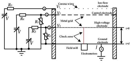
Figure 1.
Schematic diagram of the calibration apparatus.
The electric field E between the high-voltage electrode and the ground electrode can be calculated via the following Formula [17]:
where E0 is the electric field intensity at z = 0, ɛ0 is the vacuum dielectric constant, J is the ion current density, k is the ionic mobility, z is the distance away from the high-voltage electrode. The potentials at z = 0 and z = d, as shown in Figure 1, are V3 and 0, respectively, and d is the distance between the high-voltage electrode and the ground electrode. The relationship between E0, k, and J can be obtained as follows:
When the ion current density of the parallel plate electrode area is limited with space charge, E0 = 0, then
where Js is the saturated ion current density when k is substituted into Equation (3):
The space charge density ρ can be obtained via Formula (6).
The electric field at the center of the ground electrode is 1.5V3/d. The value of k depends on the measurement of Js for a specific V3, and can be obtained via Equation (4).
2.2. Simulation Model of the Calibration Apparatus
The electric field strength of the ion flow field in the calibration zone can be described by the Poisson’s formula as follows [20]:
where np and nn are the number densities of positive ions and negative ions, respectively. The continuity equations for the ion current are [20] as follows:
where Dp = 3.8 × 10⁻⁶ m2/s and Dn = 4.2 × 10⁻⁶ m2/s are the positive and negative ion diffusion coefficients, respectively. R is the positive and negative ion recombination coefficients of 1.602 × 10⁻¹⁹ C, and u+= k+E and u− = k−E are the positive and negative ion drift velocities, where k+ = 1.5 × 10⁻⁴ m2/(V·s) and k− = 1.7 × 10⁻⁴ m2/(V·s) are the positive and negative ion mobilities, respectively [20]. When there is only a positive or negative unipolar source in the field, Formulas (8) and (9) can be expanded as Formulas (10) and (11), and q+ and q− are the positive and negative ion diffusion mass fluxes, respectively.
It is obvious that there is only the divergence of the drift velocity in the field, and not the recombination of the positive and negative ions. The unipolar source was used to calibrate the probes in the simulation.
The diagram of the simulation model is shown in Figure 2. The radius of the four-layer electrode is 0.7 m, the spacing between the ion flow electrodes is 5 cm, the spacing between the control electrodes is 2.5 cm, the mesh-opening size of the high-voltage electrode is 1.25 cm, and the distance between the ion flow electrode and the control electrode and the distance between the control electrode and the high-voltage electrode are both 15 cm. The initial distance between the high-voltage electrode and the ground electrode is 15 cm, which can be changed. However, the ratio of the gap distance to the radius of the high-voltage electrode needs to be greater than 0.6 to ensure that there is no influence from electrode edge effects [6]. Since the calculation model used in this paper is basically consistent with the calculation model in [20], it can be demonstrated that the correctness of the simulation model can accurately calculate the distribution characteristics of space charges in the calibration apparatus. The boundary conditions of the electric field satisfy the following equation:
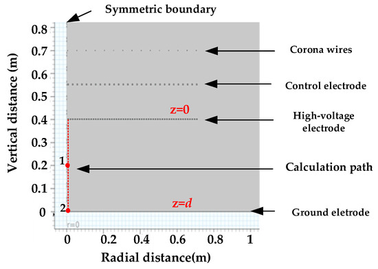
Figure 2.
Diagram of the simulation model of the calibration apparatus.
The first three boundary conditions are the potential on the ion current electrode, control electrode, and high-voltage electrode, respectively. The fourth boundary condition is the potential on the grounding plate and the outer boundary of the computational space, which is 0, and the computational space is 4 times the simulation model size. The calibration is a presented in a cylindrical shape, and in order to reduce the computational complexity, a centrally symmetric model is constructed, with calculation results of the symmetric model, which is basically consistent with that of the overall model in [20].
In addition, in order to better describe the impact of the calibration device on the calibration results of the electric field measurement device, the relative error YE is defined as Formula (13).
where E1 is the simulation calculation result and E2 is the theoretical calculation result. When YE > 0, it indicates that the control electrode voltage is too high, resulting in more ions entering the calibration area than the number of ions required for the high-voltage plate to reach saturation. When YE < 0, this indicates that the number of ions entering the calibration area cannot reach the number of ions required for the high-voltage plate to reach saturation.
3. Simulation Results and Analysis
One type of DC electric field measurement device is used for ground DC synthetic electric field measurement and is placed under the grounding electrode plate for calibration, and the surface on the scene is level with the grounding plate. The other type is a DC electric field measurement device that is used in space, which needs to be placed in the calibration area. Therefore, this article mainly analyzes the difference between the simulated values and the theoretical values of the electric field at z = d/2 and z = d in the calibration area caused by the calibration device itself, which is the error caused by the calibration device itself. Because the results of positive and negative polarity are consistent in simulation, and only differ in polarity, only the negative polarity is simulated and analyzed in this article. Although this study is based on a one-dimensional model, the research results are also applicable to three-dimensional sensors. When calibrating a three-dimensional sensor, the three sensitivities can be calibrated separately, and multiple experiments can be conducted using the three-dimensional decoupling calibration method to obtain the calibration coefficients for three-dimensional sensors [21].
3.1. Influences of the Voltage of the Ion Flow Electrode and the Control Electrode
The voltage of the ion flow electrode V1 was changed to the four values of −20 kV, −30 kV, −40 kV, and −50 kV, respectively, while V2 = −15 kV and V3 = −1.5 kV. The calculation results are shown in Figure 3. The relative errors of E are only significant near the high-voltage electrode, i.e., near z = 0, where the maximum relative errors are 6% and 7.8%, respectively. However, it can be seen that the simulation results of the electric field and space charge density on the centerline of the calibration area at the range of z = 0.04~0.15 m agree well with the theoretical calculation values, with the relative error of E being less than 0.5%.
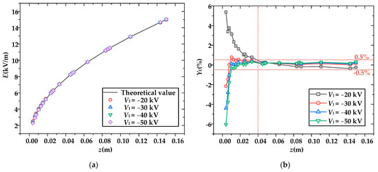
Figure 3.
Comparison of the theoretical and simulated values of the electric field under different ion flow electrode voltages: (a) electric field strength; (b) relative error.
According to Equation (3), if E0 = 0 kV/m, the calculated charge density tends to infinity, which is inconsistent with reality. Therefore, the electric field strength near z = 0 can only approach zero, resulting in a relatively large error in charge density, and the electric field strength and space charge density at each field point slightly increase with the increase in the amplitude of the applied voltage. The applied voltage V1 changes the severity of corona onset, and after corona onset, due to its higher electric field strength, the movement speed of ions accelerates. In addition, since lateral shielding is not considered in the simulation, there are ions drifting into the field from both sides, resulting in a slight increase in electric field strength and space charge density. Overall, after comprehensive corona onset in the ion flow electrode, there is a little influence of the voltage of the ion flow electrode on the electric field and charge distribution within the calibration area.
In order to ascertain the influence of the control electrode voltage, we maintained V1 = −30 kV and V3 = −1.5 kV, while varying the control electrode voltage V2 to −15 kV, −10 kV, −5 kV, −3 kV, and −2 kV. The calculation results are shown in Figure 4. It can be seen that the voltage of the control electrode has a significant impact. As the voltage of the control electrode continues to increase, the simulated value of the electric field intensity at z = 0 gradually decreases. When the applied voltage of the control electrode is lower, the ion movement speed slows down, with the speed becoming insufficient to make the electric field intensity of the high-voltage electrode plate approach zero. The charges in the field are not saturated, which means that they cannot distribute the field according to the theoretical calculation values. Therefore, a larger value of control electrode voltage is required so that the field tends to be saturated, thus fitting better with the theoretical values. When V2 = −15 kV, the field calculation results have a small deviation from the theoretical values. Therefore, the electric field intensity and charge density in the field deviate significantly from the theoretical values.
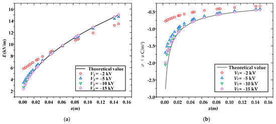
Figure 4.
Comparison of the simulated and theoretical values of the electric field and space charge density under different control electrode voltages: (a) electric field strength; (b) charge density.
3.2. Influence of the Voltage of the High-Voltage Electrode
The V1 = −25 kV and V2 = −15 kV were maintained, and V3 was changed to −0.75 kV, −1.5 kV, −3 kV, and −4.5 kV, respectively. The variations in the electric field and charge density with the change in the nominal field strength of the calibration gap are shown in Figure 5; En = V3/d represents the nominal field strength in the calibration area. It can be seen that the difference between the simulated and theoretical values of electric field strength and charge density increases with the increase in the nominal field strength. The main reason is that as the nominal field strength increases, the charge density in the calibration area is insufficient to achieve E0 = 0, leading to a significant discrepancy between the theoretical and simulated values.
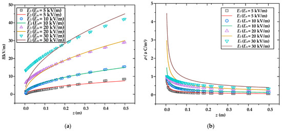
Figure 5.
Comparison of simulated and theoretical values of electric field and space charge density under different electric field En: (a) electric field strength; (b) charge density.
To verify this, a constant ΔV = V1 − V2 was maintained, and the voltage of the control electrode V2 was increased. The relative errors of E in the calibration area at nominal field strengths En = 7.5 kV/m and En = 30 kV/m as a function of V2 were calculated, and are shown in Figure 6. From Figure 6a, it can be seen that the relative error of E increases with the increase in the control electrode voltage and changes from a negative value to a positive error when En = 7.5 kV/m. When the control electrode voltage is too high, it can lead to oversaturation of the charge density in the calibration area. That is, the simulated value of E becomes larger than the theoretical value. Therefore, it can be concluded that the relative error of E can be kept at essentially zero by reasonably adjusting the control electrode voltage at low field strengths. This conclusion is consistent with the results of theoretical and measured values presented in the literature [18,19]; therefore, it can also be concluded that an optimal range exists for electric field calibration in the calibration device. From Figure 6b, it can be seen that, when En = 30 kV/m, the relative error of E also increases exponentially with the increase in the control electrode voltage, but it does not cross zero. Exponential fitting was used to fit the two curves in Figure 6b, and the trends of the relative error of E between the simulated and theoretical values of the electric field strength as a function of V2 are shown in Equations (14) and (15):
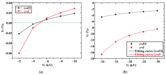
Figure 6.
The relative errors of simulated values of electric field at z = d and z = d/2 changes with V2: (a) En = 7.5 kV/m; (b) En = 30 kV/m.
The values of R2 are both 1, and the formula indicates that the error of E tends infinitely towards a stable value less than 0. That is, the charge density entering the calibration area reaches saturation under high field strength. However, considering the limitations of the insulation strength between the plates, the control electrode voltage cannot be applied indefinitely, and because of the ion mobility, tends to be saturated with an increase in the voltage of the high-voltage electrode. Indeed, when the voltage of V3 is more than 0.5 kV, the ion mobility of the negative ions is already saturated [17]. Therefore, even though the charge density reaches saturation under a high field strength, it is impossible to make E0 = 0.
The electric field E in the calibration zone at different times is shown in Figure 7a; the electric field strength gradually stabilized after 0.4 s. The variations in E0 with time are shown in Figure 7b under different electric field intensities. It can be seen that the stable value of E0 increases with an increase in the En. Even under low field strengths, E0 ≠ 0, and it can only approach 0. The increase in the electric field strength leads to a larger relative error. Furthermore, the simulated and theoretical values of the saturation space charge density with V3 are shown in Figure 8. It can be seen that the theoretical value of saturated charge density varies linearly with V3, while the simulated value of the saturation charge density gradually saturates with an increase in V3. This further explains the reason for the larger relative error. Therefore, when calibrating an electric field measuring device using a four-plate ion flow generator, the calibrated electric field range should be set at a lower electric field intensity.
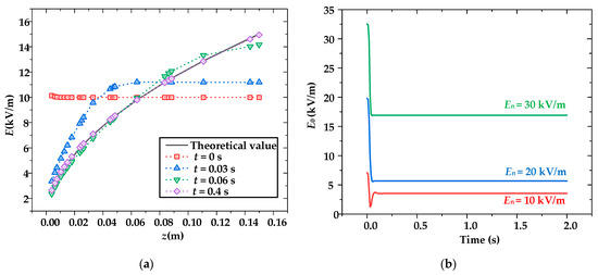
Figure 7.
The variation in the stable value of E0 with time. (a): E over time; (b) E0 over time.
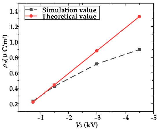
Figure 8.
The variation in theoretical and simulated values of saturation current density with electric field intensity.
3.3. Influence of the Distance Between the High-Voltage Electrode and the Ground Electrode
Keeping V1 = −25 kV, V2 = −15 kV, and V3 = −5 kV constant, the gap distance d was changed to 20 cm, 30 cm, 40 cm, and 50 cm, respectively. The impact of the gap distance on the electric field and charge density distribution is shown in Figure 9. It can be seen that the theoretical and simulated values of electric field strength and charge density exhibit a trend of first decreasing and then increasing with the increase in gap distance. Since the applied voltage is the same, the electric field strength varies with the gap distance, with larger gaps having smaller fields. According to the analysis in the previous section, the greater the electric field strength, the larger the relative error of E.
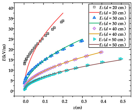
Figure 9.
Comparison of the simulated and theoretical values of the electric field with different gap distances at the same voltage.
For further analysis of the influence of the gap distance d, the voltages of the high-voltage electrode V3 for the gap distances of 20 cm, 30 cm, 40 cm, and 50 cm were set to −2.5 kV, −3.75 kV, −5 kV, and −6.25 kV, respectively, and the different gap distances d maintained a constant nominal field strength of En = 12.5 kV/m. The electric field distribution in the calibration area and the relative error are shown in Figure 10. It can be seen that the errors under different gaps with En = 12.5 kV/m are relatively small, and they can be controlled in less than 3%, with d = 0.15~0.5 m. Therefore, this further confirms that the electric field strength is the main factor affecting the calibration error.
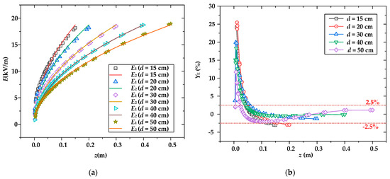
Figure 10.
Comparison of simulated and theoretical values of the electric field under the same nominal field and different gap distances: (a) electric field distribution; (b) relative error.
Furthermore, the relative errors of E at z = d and z = d/2 were calculated under different field intensity levels of 5 kV/m, 10 kV/m, 20 kV/m, and 30 kV/m, and the calculation results are shown in Table 1 and Table 2, respectively. In the tables, positive values indicate oversaturation of ion density in the calibration area, while negative values indicate undersaturation of ion charge density. From the table, it can be seen that as the field strength increases, the degree of undersaturation of charge density in the calibration area will increase. This also indicates that it is difficult to reach a saturation state at high field strengths, resulting in an increase in calibration errors. Conversely, it can be observed from Table 1 and Table 2 that the relative error of electric field intensity at z = d and z = d/2 decreases with the increase in the electric field intensity. However, the absolute values of the relative error of electric field intensity at z = d and z = d/2 have a trend of first decreasing and then increasing as the En increases. This finding is consistent with the previous conclusion obtained for d = 15 cm, and shows that an optimal electric field intensity with the smallest relative error exists. The relative error of electric field intensity in the calibration area is minimal when En is about 10 kV/m. From Table 1, the relative error of E at z = d/2 can be controlled to less than 4%. From Table 2, the relative error of E at z = d increases with an increase in the gap distance.

Table 1.
The relative error between the simulated and theoretical values of the electric field at z = d/2.
Table 2.
The relative error between the simulated and theoretical values of the electric field at z = d.
From the above analysis, it can be seen that there is, in fact, an optimal electric field calibration range for calibration devices with different gap distances, in which the calibration error caused by the calibration device itself can be controlled within a certain range.
Taking gap distances of 15 cm and 50 cm as examples, and controlling the relative error of the electric field to be less than 5%, the optimal calibration range of the electric field intensity is analyzed. Assuming that calibration is performed at z = d, further analysis for d = 15 cm and d = 50 cm reveals that the relative error of the electric field varies with the electric field, as shown in Figure 11. It can be seen that when the field strength is below 10 kV/m, the absolute value of the relative error of d = 15 cm is smaller than that of d = 50 cm. However, when the field strength reaches 30 kV/m, the absolute value of the calibration error of d = 15 cm is larger than that of d = 50 cm, which is the reverse as with low field strength. Therefore, an optimal electric field calibration position for the actual calibration device for different gap distances exists. Exponential fitting was used to fit the error variation curves, as shown in Figure 11. The fitting formulas for the relative calibration error with field strength En for d = 15 cm and d = 50 cm are shown in Formulas (16) and (17), respectively.
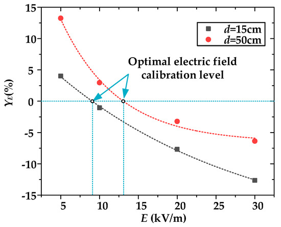
Figure 11.
Relative error of electric field at z = d changes.
The values of R2 are both 1. From the fitting formula of the relative error of E, when the calibration error is controlled to be less than 5% the optimal of calibration electric field levels are in the range of 4~15 kV and 9~24 kV, respectively., and the optimal calibration electric field levels are about 8 kV/m and 15 kV/m, respectively. The variation in the optimal electric field calibration level with the gap distance is shown in Figure 12, which is the level of the electric field when the error between the simulated and theoretical values of the electric field intensity at z = d is zero. It can be seen that the optimal electric field calibration level increases with the increase in gap distance when d is more than 20 cm.
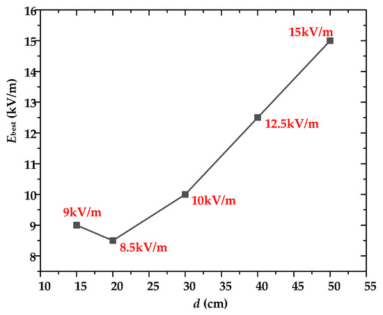
Figure 12.
The optimal electric field calibration changes with gap distance.
In addition, the electric field distribution in the vertical direction of the different gap centers with En = 30 kV/m is shown in Figure 13. It can be seen that there is an intersection point between the simulated and theoretical values of the electric field, which indicates that the simulated and theoretical values are identical at this location. Therefore, we can define this point as the optimal location for electric field calibration, and the variation in the optimal calibration position with gap distance is shown in Figure 14. It can be seen that the height of the optimal calibration position increases linearly with an increase in the gap distance, and the optimal position is always located at a height of 0.4d from the grounded plate.
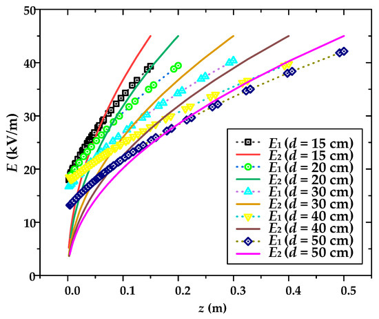
Figure 13.
The simulated and theoretical values of the electric field in the vertical direction of the different gap centers when En = 30 kV/m.
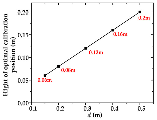
Figure 14.
The height of the optimal calibration position varies with gap distance.
4. Conclusions
A simulation model of the generator of a DC electric field with space charge is established based on a dilute substance transfer model and an electrostatic field model. It is used to calculate and analyze the influence of the applied voltages of the ion flow electrode, control electrode, and high-voltage electrode, as well as the influence of the gap distance in the calibration area on the electric field calibration results. The simulation results indicate that the influence of the ion flow electrode voltage on the calibration can be neglected when the corona wire is fully charged, while the control electrode voltage plays a decisive role in determining the electric field and charge density. The relative error of the electric field at z = d and z = d/2 decreases with the increase in the electric field intensity; however, the absolute values of the calibration errors of electric field intensity at z = d and z = d/2 have a trend of first decreasing and then increasing as the En increases. The relative error of the electric field at z = d/2 can be controlled in less than 4%, and the relative error of the electric field at z = d increases with the increase in the gap distance. For different gap distances, an optimal calibration range of electric field and an optimal calibration position exist, both of which increase with the increase in gap distance, and the optimal calibration position is located at a distance of 0.4d from the ground electrode.
Author Contributions
Conceptualization, W.S. and Y.W.; methodology, M.D.; software, X.K.; validation, J.Z. and C.Z.; formal analysis, W.X.; investigation, Z.S.; writing—original draft preparation, W.S., Z.S., M.D., X.K., J.Z., C.Z., W.X. and Y.W.; writing—review and editing, W.S., Z.S., M.D., X.K., J.Z., C.Z., W.X. and Y.W. All authors have read and agreed to the published version of the manuscript.
Funding
This research was funded by the Science and Technology Project of State Grid Henan Electric Power Company, grant number 52170224001P.
Data Availability Statement
The original contributions presented in the study are included in the article. Further inquiries can be directed to the corresponding author.
Conflicts of Interest
Authors Wei Song, Xiaokuo Kou, Jiatao Zhang and Chaofeng Zhang were employed by the State Grid Henan Electric Power Company. Authors Manling Dong, Weifeng Xin and Zeyan Shi were employed by the State Grid Henan Electric Power Research Institute. Author Yanzhao Wang was employed by the company China Electric Power Research Institute and State Key Laboratory of Power Grid Environmental Protection. The authors declare that this study received funding from State Grid Henan Electric Power Company. The authors declare that the research was conducted in the absence of any commercial or financial relationships that could be construed as a potential conflict of interest.
References
- Maruvada, P.S. Corona Performance of High-Voltage Transmission Lines; Research Studies Press: London, UK, 2000. [Google Scholar]
- Liu, Z. UHV AC/DC Power Grid; China Electric Power Press: Beijing, China, 2013. [Google Scholar]
- Zhao, W. HVDC Engineering Technology; China Electric Power Press: Beijing, China, 2004. [Google Scholar]
- Taylor, D.M. Measuring techniques for electrostatics. J. Electrost. 2001, 51–52, 504–508. [Google Scholar] [CrossRef]
- Zhao, L.; Cui, X.; Lu, J.Y.; Xie, L.; Cui, Y. Discussion on Measurement Method of Total Electric Field for DC Transmission Lines. Proc. CSEE 2018, 38, 644–695. [Google Scholar]
- IEEE Standard 1227-1990; IEEE Guide for the Measurement of DC Electric-Field Strength and Ion Related Quantities. IEEE: Piscataway, NJ, USA, 2010.
- Maruvada, P.S.; Dallaire, S.R.D.; Pedneault, R. Development of Field-Mill Instruments for Ground-Level and Above-Ground Electric Field Measurement under HVDC Transmission Lines. IEEE Power Eng. Rev. 1983, PER-3, 42–43. [Google Scholar] [CrossRef]
- Parizotto, R.A.; Mesquita and Porto, R.W. Design and calibration of an atmospheric electric field sensor with wireless communication. In Proceedings of the 2015 International Symposium on Lightning Protection (XII SIPDA), Balneario Camboriu, Brazil, 28 September–2 October 2015; pp. 69–74. [Google Scholar]
- Tant, J.P.; Bolsens, B.; Sels, T.; Dommelen, D.; Driesen, J.; Belmans, R. Design and application of a field mill as a high-voltage DC meter. IEEE Trans. Instrum. Meas. 2007, 56, 1459–1464. [Google Scholar] [CrossRef]
- Cui, Y.; Song, X.; Wang, C.; Zhao, L.; Wu, G. Ground-level DC electric field sensor for overhead HVDC/HVAC transmission lines in hybrid corridors. IET Gener. Transm. Distrib. 2020, 14, 4173–4178. [Google Scholar] [CrossRef]
- Cui, Y.; Yuan, H.; Song, X.; Zhao, L.; Liu, Y.; Lin, L. Model, design, and testing of field mill sensors for measuring electric fields under high-voltage direct-current power lines. IEEE Trans. Ind. Electron. 2017, 65, 608–615. [Google Scholar] [CrossRef]
- Chu, Z.; Yang, P.; Wen, X.; Peng, C.; Liu, Y.; Wu, S. A MEMS-based Electric Field Sensor with Self-compensation for Sensitivity Drift. J. Electron. Inf. Technol. 2023, 45, 3040–3046. [Google Scholar]
- Wang, X.J.; Zhang, J.; Chen, F. Design of Miniature Integrated Optical Waveguide Electric Field Sensor. Chin. J. Sens. Actuators 2021, 50, 67–75. [Google Scholar]
- Wang, Y.; Xu, J.; Gan, Z. Analysis of influencing factors for measurement of total electric field on residential platform nearby DC transmission line. Adv. Technol. Electr. Eng. Energy 2021, 34, 1445–1450. [Google Scholar]
- Ya, M.; Yu, Z.; Fan, Y.; Zhang, B.; Zhang, C.; Wang, X.; Zeng, R.; He, J. Calibration of a sensor for an ion electric field under HVDC transmission lines. J. Eng. 2019, 3, 2842–2845. [Google Scholar] [CrossRef]
- Fritzen, C.L. Electric Field Sensor Calibration Using Horizontal Parallel Plates. In Proceedings of the 2019 International Symposium on Lightning Protection (XV SIPDA), So Paulo, Brazil, 30 September–4 October 2019; pp. 1–5. [Google Scholar]
- Wang, Y.; Zhang, J.; Gan, Z.; Xu, J. Simulations and experiments of the generation apparatus of the DC electric field with the space charge. High Volt. 2021, 6, 1061–1068. [Google Scholar] [CrossRef]
- Liang, X. Development of calibration apparatus for DC electric field measurement device. In Proceedings of the 2016 EEE International Conference on High Voltage Engineering and Application (ICHVE), Chengdu, China, 19–22 September 2016; pp. 1–3. [Google Scholar]
- Zhang, B.; Wang, W.; He, J. Impact factors in calibration and application of field mill for measurement of DC electric field with space charges. CSEE J. Power Energy Syst. 2015, 1, 31–36. [Google Scholar] [CrossRef]
- Wan, B.; Gan, Z.; Xie, H.; Qi, P.; Xu, J. Calibration Analysis of Field Mills in the Space Charge Modified Field above Ground Based on Convection-diffusion Equation. In Proceedings of the 2021 International Conference on Power System Technology (POWERCON), Haikou, China, 8–9 December 2021; pp. 2229–2235. [Google Scholar]
- Zhao, Z.; Li, Y.; Yang, X.; Luo, C. Three-dimensional electric field sensor with low inter-axis coupling. J. Meas. Sci. Instrum. 2024, 15, 95–104. [Google Scholar] [CrossRef]
Disclaimer/Publisher’s Note: The statements, opinions and data contained in all publications are solely those of the individual author(s) and contributor(s) and not of MDPI and/or the editor(s). MDPI and/or the editor(s) disclaim responsibility for any injury to people or property resulting from any ideas, methods, instructions or products referred to in the content. |
© 2025 by the authors. Licensee MDPI, Basel, Switzerland. This article is an open access article distributed under the terms and conditions of the Creative Commons Attribution (CC BY) license (https://creativecommons.org/licenses/by/4.0/).