Hybrid Deep Learning for Predictive Maintenance: LSTM, GRU, CNN, and Dense Models Applied to Transformer Failure Forecasting

Abstract

Data is an important resource for gaining knowledge about the behavior and condition monitoring of machines, enabling the estimation of parameters and the prediction of failures. However, in industrial environments, sensor interruptions often create gaps in the time series, which affects the reliability of the data. To overcome this challenge, this paper proposes an imputation strategy based on recurrent neural networks, in particular long short-term memory (LSTM) models, within a multivariate encoder–decoder architecture. This approach utilizes correlations between variables to reconstruct missing values, resulting in more complete and robust datasets. Experimental results with multivariate time series show that the proposed method achieves accurate imputation, with errors as low as RMSE = 2.33 and $R^2$ = 0.90 for some variables. Comparisons with alternative architectures, including GRU and Dense networks, show that LSTM excels in specific cases (e.g., VL3, $R^2$ = 0.45), while the Dense architecture provides more stable performance across most variables. In particular, the Dense model achieved the best overall balance between accuracy and robustness, reaching RMSE = 2.33 and $R^2$ = 0.90 for the best-performing variables, while the LSTM achieved the lowest error values in targeted scenarios, confirming its suitability for capturing complex temporal dependencies. Overall, this study highlights the feasibility of using recurrent neural networks to exploit temporal correlations for reliable data recovery, even under conditions of signal interruption in factory environments.

1. Introduction

The strategic management of a company in the industrial sector is directly related to the efficient administration of its resources, with the aim of overcoming the challenges of adaptability and flexibility demanded by the dynamic market. Within this context, key areas such as physical asset management play a fundamental role, as their high performance directly impacts the organization’s operational response capacity and the quality of the services offered [1,2]. Also, physical asset management is used to treat equipment as strategic assets, as they generate value for the company when kept fully operational [3]. This operational efficiency is guaranteed by preventive maintenance (in accordance with manufacturers’ guidelines) and a well-structured maintenance management system that ensures the availability and reliability of resources [4].

With the advance of digitalization and the increase in computing power, predictive maintenance has become a strategic ally, thanks to models based on data analysis that make it possible to predict failures and plan interventions in both the short and long term [1,5,6,7,8,9,10].

The shift towards predictive maintenance, exemplified by Prognosis and Health Management (PHM) and Condition-based Maintenance (CBM), is facilitated by emerging technologies such as IoT, cloud computing, and advanced data analytics [11,12]. Industry 4.0 technologies are revolutionizing maintenance tasks and management strategies, promoting innovations like remote maintenance and self-maintenance [13,14].

Data-based maintenance makes it possible to identify hidden patterns in equipment, such as abnormal vibrations, temperatures outside the ideal range, or irregular energy consumption [15,16]. According to McKinsey [17], in ”A Review on Machinery Diagnostics and Prognostics Implementing Condition-Based Maintenance”, the integration of IoT sensors and machine learning algorithms transforms raw data into actionable insights, increasing operational reliability and reducing repair costs by up to 25%.

Intelligent Asset Management Platforms (IAMPs) are crucial in this transformation, integrating maintenance with other departments to conserve asset value and improve services. These platforms should support a strategic view of asset management, considering business priorities in work and investments [18].

Predictive analysis also makes it possible to optimize human and material resources. A study by McKinsey [17] points out that companies that adopt data management platforms in maintenance are able to reallocate up to 40% of the workforce to strategic activities, rather than emergency fixes. This reinforces the role of data not just as a technical tool, but as a strategic element for organizational efficiency.

According to Zhang and Feng [19,20] in data-driven safety management in industrial environments, the correlation between operational variables and critical events can reduce accidents by up to 50%, contributing to safer working environments.

Integrating data into management systems creates an intelligent ecosystem where decisions are based on evidence. As highlighted by Dalzochio et al. [21] in “Machine Learning and Reasoning for Predictive Maintenance in Industry 4.0”, the combination of big data and artificial intelligence makes it possible not only to predict failures, but also to simulate scenarios and prioritize actions based on technical and economic criteria.

The purpose of this study is to analyze the data of a transformer whose information base is incomplete. To this end, an AI-based approach is followed, using deep learning techniques with a multivariate encoder–decoder architecture to fill in the missing data. Statistical techniques are then applied to validate the data generated by the network at intervals with missing information. In addition, supervised and unsupervised learning techniques are used for frequency analysis and fault classification to detect patterns and support predictive maintenance.

This article is organized as follows: Section 2 reviews the state of the art in imputation and normalization of data in time series; Section 3 describes the proposed methodological approach based on LSTM networks with a multivariate encoder–decoder architecture; Section 4 presents the dataset, the results of the imputation, and the statistical analysis; and Section 5 discusses the main results, limitations, and directions for future research. Finally, Section 6 summarizes the conclusions of this study.

2. Literature Review

In the production process, it is crucial to keep the equipment in good condition. High availability and less production downtime are favored by proper maintenance and service [22,23]. On the other hand, maintenance costs are a major financial burden for power plants. Therefore, it is crucial to minimize maintenance costs while achieving satisfactory production results. The European Standard EN 13306 [24] defines maintenance as the sum of all technical, managerial, and administrative actions taken throughout the life cycle of an object to keep it in a condition or restore it to a condition in which it can perform its intended function. Therefore, routine maintenance, condition monitoring, inspections, parts replacement, repairs, overhauls, and planning are all part of maintenance.

There is extensive research on predictive maintenance (PdM), also known as “online monitoring”, “risk-based maintenance”, or “condition-based maintenance”, which has evolved from visual inspection methods to automated procedures through the use of sophisticated signal processing techniques based on pattern recognition, machine learning, neural networks, fuzzy logic, etc. [15,25,26,27].

The challenges of industry are increasingly linked to the challenges of scientific research. The arrival of Industry 4.0 brings numerous advantages for companies, allowing them to monitor their processes more precisely and efficiently. This is possible thanks to the use of intelligent sensors, such as temperature, pressure, humidity, vibration, and proximity sensors, computer vision cameras, and acoustic sensors, in addition to traditional IoT sensors [28,29].

2.1. Data Cleansing and Imputation

Sensor readings are often noisy and prone to errors due to poor sensor quality and random environmental effects [16]. Elnahrawy [30] proposed a Bayesian approach that combines prior knowledge of the actual sensor readings, the sensor’s noise characteristics, and the observed noisy measurements. However, in practice, it is often difficult or even impossible to accurately determine the noise characteristics of a sensor [31,32,33].

These studies address the challenges of data cleaning and outlier detection in sensor networks. Kalman filters are a widely used approach, leveraging spatial and temporal dependencies in sensor data to effectively identify and correct outliers [34]. Tan et al. [35] also explored regression techniques, highlighting the potential of high-order polynomials for datasets with low variability. Shao et al. [36] proposed a method based on multisensor spatiotemporal correlation, which outperformed traditional techniques such as moving averages and stacked denoising autoencoders. Liu et al. [37] developed an online outlier resistant filter cleaner that integrates an adaptive process model estimate with a modified Kalman filter. This method offers key advantages, including no requirement for prior model knowledge and effectiveness with autocorrelated data. Collectively, these approaches underscore the value of exploiting spatial and temporal correlations in sensor data for robust cleaning and outlier detection, with Kalman filter-based methods consistently demonstrating strong performance.

The presence of missing values, noise, and outliers can significantly undermine the integrity of time-series data. Hyndman and Athanasopoulos [38] recommend classical imputation techniques, such as linear interpolation and moving averages, because of their simplicity and low computational cost. However, these methods assume that data patterns are linear or change smoothly over time, which often does not reflect the complexity of real-world series.

Keogh and Kasetty [39] highlight a major challenge in the field: the lack of standardized benchmarks, which makes it difficult to rigorously compare the performance of different imputation methods. Esling and Agon [40] reinforce the need for robust outlier detection strategies, proposing adaptations of the DBSCAN algorithm to better handle the non-stationary nature of many time series.

In recent years, more flexible approaches based on semi-supervised learning and probabilistic modeling—such as imputed k-NN and expectation maximization (EM)—have gained traction, particularly in scenarios involving Missing Not At Random (MNAR) data, where traditional methods tend to fall short [41,42,43,44,45].

2.2. Standardization and Transformation

Data normalization significantly impacts the performance of machine learning algorithms, particularly k-NN and SVM. For k-NN, studies show that different normalization techniques yield varying results across datasets [46,47]. L2-Norm, Decimal, and TFIDF methods often perform well for k-NN [46]. Min–max normalization generally outperforms Z-score for k-NN in terms of accuracy [48]. However, the choice of scaling method should be based on specific dataset characteristics [47]. For SVM, min–max normalization consistently improves performance, while its effect on k-NN can vary depending on the dataset’s statistical properties [49]. The impact of normalization aligns with the mathematical concepts of different algorithms, with SVM showing consistent improvement, ANN showing no significant change, and k-NN’s performance varying based on dataset properties [49]. These findings emphasize the importance of selecting appropriate normalization techniques for specific algorithms and datasets.

2.3. Bibliometric Analysis and Review of Recent Literature

Figure 1 shows a bibliometric analysis using the keywords: fault detection AND machine learning AND signal processing. A strong relationship can be observed among the documents produced in the areas of asset management, maintenance, systems, and industrial engineering. These domains currently treat data quality as a strategic pillar for decision making.

There is a wide range of articles that address the importance of predictive maintenance and the use of supervised and unsupervised learning techniques to support decision making in machine interventions before failures occur. Based on this, an analysis was performed on the 200 articles found using the previously defined keywords. From this analysis, the most relevant articles in the field of predictive maintenance using machine learning techniques were selected based on the following criteria:

• Publication year equal to or later than 2019, in order to focus on recent advances in the state of the art.
• Minimum of 10 total citations, ensuring a basic level of impact and recognition in the scientific community.
• Citations per year used as the main metric of relevance, to highlight influence proportional to the time since publication.

Table 1. Bibliographic analysis state of the art in fault detection using machine learning and signal processing.

Authors	Year	Full Title	Main Technique	Source	Cit./Year
[50]	2021	A review on fault detection and diagnosis techniques using machine learning	Systematic Review	Springer	101.25
[51]	2022	An explainable artificial intelligence approach for fault detection	XAI + ML	Elsevier	98.33
[52]	2023	Application of machine learning methods in fault detection	SVM, DWT, CNN	Springer	70.00
[53]	2020	Multisensor data fusion for gearbox fault diagnosis using deep learning	Data Fusion + CNN	Elsevier	69.00
[54]	2019	1-D convolutional neural networks for signal processing applications	1D CNN	IEEE	66.67
[55]	2022	Physics-Informed LSTM hyperparameters selection for robust fault detection	LSTM + Physics Models	Elsevier	65.33
[56]	2019	Machine learning-based fault diagnosis for synchronous motors	Autoencoder + DNN	IEEE	58.67
[57]	2021	Review on machine learning algorithms for fault detection in electrical machines	ML Review	Academia.edu	55.25
[58]	2023	Challenges and opportunities of deep learning-based predictive maintenance	Deep Learning	Springer	52.00
[59]	2021	Machine learning-based fault detection in electric vehicles using vibration signals	Data-Driven ML	MDPI	48.75

shows the results of the articles that fulfill the criteria set for their selection. Based on the analysis of these works, the following recurring limitations were identified: (i) real-time integration is under-researched, with most studies relying on offline or simulated data; (ii) model explainability (XAI) is only considered by a fraction of publications, although it is a critical factor in industrial contexts; (iii) effective strategies are still lacking for processing sparse and noisy data, with only a few articles addressing unbalanced or incomplete datasets; (iv) model validation takes place predominantly in controlled or academic environments, with little practical application; (v) there is a gap in interoperability between domains, with little knowledge transfer between different systems or industry sectors; and (vi) hybrid techniques that combine physical models with machine learning are still under-researched.

3. Methodology

This section describes the detailed methodology employed to address incomplete multivariate time series from power transformers. The proposed approach combines data preprocessing, deep-learning-based imputation, frequency-domain analysis, clustering, and forecasting to support predictive maintenance.

The dataset was organized in a DataFramefrom the Pandas library, with measurement timestamps in the first column. Initially, the column format was verified as datetime. Each record was segmented by day, using an auxiliary column containing only the date and grouped via groupby(). Daily groups were stored as separate DataFrames for independent analysis. Duplicate records were removed, and the DataFrames were reindexed to maintain temporal consistency.

Missing values and outliers were preliminarily identified. Outliers were flagged using statistical thresholds (e.g., values beyond 3 standard deviations) and inspected in combination with domain knowledge, ensuring the subsequent models were trained on robust data [38].

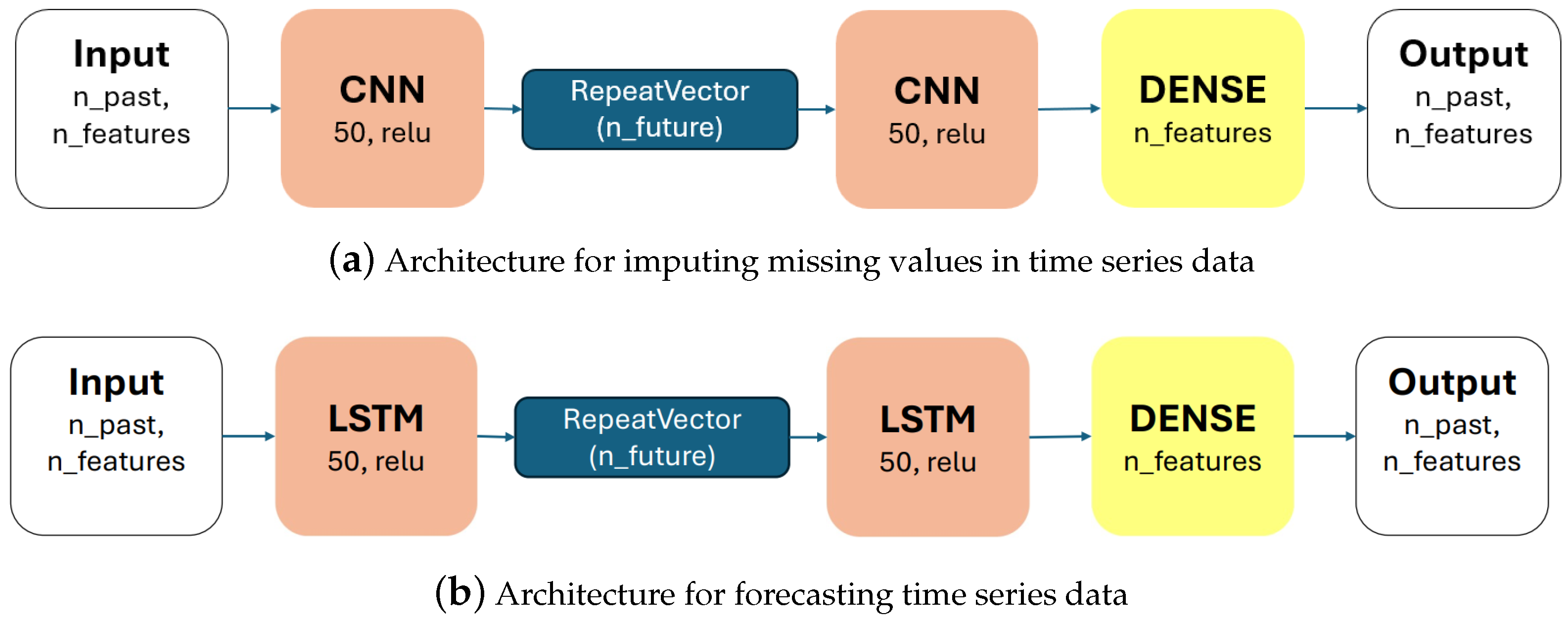
The core of the imputation strategy employs a multivariate encoder–decoder architecture with three alternative models: LSTM, GRU, and CNN. The dataset $X\in {\mathbb{R}}^{T\times F}$, with T time steps and F variables, is divided into sliding windows of length L (lookback parameter).

Each input sequence is defined as follows:

$${\mathbf{X}}_i=[x_i,x_{i+1},\dots ,x_{i+L-1}]\in {\mathbb{R}}^{L\times F},$$

(1)

with the target being the next time step:

$${\mathbf{y}}_i=x_{i+L}\in {\mathbb{R}}^F.$$

(2)

The encoder (Bidirectional LSTM/GRU or CNN layers) processes the input sequence to extract temporal features and produces a context vector. The decoder (Unidirectional LSTM/GRU or Dense layers for CNN) repeats the context vector to predict the next step(s) in the sequence. The output layer is a TimeDistributed(Dense) layer reconstructing the F variables.

Training uses backpropagation through time (BPTT) with the mean squared error (MSE) loss, optimized via Adam [60]. For variables with high variability, a custom loss penalizing low variance predictions was also tested [55].

After imputing missing values, signals were transformed to the frequency domain using the fast Fourier transform (FFT). The power spectral density (PSD) was computed as follows:

$$PSD\left(f\right)={\displaystyle \frac{FFT\left(s\right)·FFT{\left(s\right)}^{*}}{N}},$$

(3)

where $FFT\left(s\right)$ represents the transform of signal s, $FFT{\left(s\right)}^{*}$ its complex conjugate, and N is the number of samples. This analysis allows the identification of dominant frequency components and potential anomalies [61].

K-means clustering was applied to group observations based on operational similarity. The number of clusters was selected using the elbow method, and the Euclidean distance to the cluster centroids was used to identify potential outliers. This step complements the frequency-domain analysis by highlighting unusual operating patterns that could indicate early faults [35].

For forecasting, a sliding window strategy was applied: 10 past steps were used to predict 20 future steps. Three architectures were evaluated:

-

GRU encoder–decoder with 64 units;

-

LSTM encoder–decoder with 64 units;

-

Dense (MLP) network with 128 hidden units.

Outputs were structured as univariate multistep predictions, trained and evaluated independently for each variable. The train–test split preserved temporal order (80% training, 20% testing). Models were trained for 30 epochs using the Huber loss function and Adam optimizer, with an initial learning rate of $1\times {10}^{-3}$, reduced progressively by 10% each epoch via a learning rate scheduler. Performance metrics include RMSE, MAPE, MAE, and $R^2$.

Initially, it was necessary to impute missing values for each variable in the dataset. This was accomplished through forecasting using the architecture shown in Figure 2a. Once the data were completed, a frequency analysis was conducted to identify potential deviations in the frequency domain. Subsequently, a cluster analysis was performed used the K-means methodology. Finally, a forecast was generated using the architecture shown in Figure 2b.

4. Experiments and Results

4.1. Power Transformer Data Processing

The dataset analyzed was collected by IoT sensors placed in transformers in operation, with measurements taken every 15 min. The variables evaluated include electrical parameters and transformer status signals.

The phase voltages are designated as VL1, VL2, and VL3, which refer, respectively, to the voltages of phase lines 1, 2, and 3. The line currents are documented as IL1, IL2, and IL3, which refer to the currents in lines 1, 2, and 3. The voltages between phases are also tracked, called VL12 (between lines 1 and 2), VL23 (between lines 2 and 3), and VL31 (between lines 3 and 1). The neutral current is measured by the INUT variable.

In addition to the electrical variables, various environmental and operating indicators are recorded. The term OTI refers to the oil temperature indicator, while the winding temperature is captured by WTI. The temperature of the environment around the transformer is indicated by ATI, while the oil level is shown by OLI. As for alarms and protection devices, the system includes the oil temperature alarm ($OT{I}_A$), automatic over-temperature activation ($OT{I}_T$), and the magnetic oil gauge alarm ($MO{G}_A$), which signals the possibility of faults associated with insulation or cooling. Figure 3 presents the data in a time series format with a 15 min sampling rate. It is noticeable that, during certain time intervals, the data remains constant, indicating possible sensor stagnation or data transmission issues.

Due to the limited processing power of the computer, the resample function of Python 3.12.7 Pandas library was used to reduce the sampling rate from 15 min to 1 h, as illustrated in Figure 4.

Table 2. Statistical parameters of power transformer variables.

Statistics	OTI	ATI	VL1	VL2	VL3	IL1	IL2	IL3	VL12	VL23	VL31	INUT
count	17,865	17,865	17,865	17,865	17,865	17,865	17,865	17,865	17,865	17,865	17,865	17,865
mean	29.77	27.06	241.04	240.42	239.76	80.75	64.61	91.25	416.72	415.69	417.27	28.88
std	11.28	5.51	9.44	9.88	8.64	35.69	37.55	36.55	17.22	15.00	16.90	13.27
min	11.00	12.00	112.60	0.00	90.10	0.00	0.00	0.00	0.00	189.50	0.00	0.00
25%	25.00	24.00	234.70	234.40	234.40	52.70	37.00	62.20	406.00	406.10	406.80	19.40
50%	29.00	27.00	243.10	242.40	241.10	73.60	53.70	85.20	420.30	418.40	420.30	27.10
75%	33.00	30.00	247.80	246.90	245.50	103.20	86.70	117.70	428.30	426.00	428.50	36.90
max	248.00	44.00	258.10	257.00	256.50	224.10	253.60	247.30	446.50	444.80	447.30	145.80

shows the statistical parameters of the data before the use of any methodology.

The performance of the models, using the architectures described above, was evaluated based on the final loss after training. The results are summarized as follows:

• LSTM: Final loss = 0.00158.
• GRU: Final loss = 0.00156.
• CNN: Final loss = 0.00120.

Among the models tested, the CNN, using the architecture described above, achieved the lowest loss, indicating the best performance for the task, with a final loss of 0.00120.

Figure 5 illustrates several variables imputed using both the traditional method and the deep learning models proposed in this study.

Table 3. Global stability of imputation methods.

Method	Mean Diff	Std Diff	Average Correlation	Stability Interpretation
CNN	1.00	0.84	0.89	High stability, consistent and accurate imputation with preserved dynamics.
KNN	0.00	1.93	0.87	Very stable; minor variability reduction but maintains overall pattern.
Mean	0.00	1.99	0.86	Statistically stable but oversmooth; tends to flatten temporal variations.
Median	0.99	1.89	0.86	Similar to mean; robust but with slight smoothing effects.
Forward fill	2.54	1.00	0.93	Strong correlation but introduces bias and systematic level shifts.

summarizes the experimental results, highlighting the best imputation outcomes obtained from tests conducted with different parameter settings.

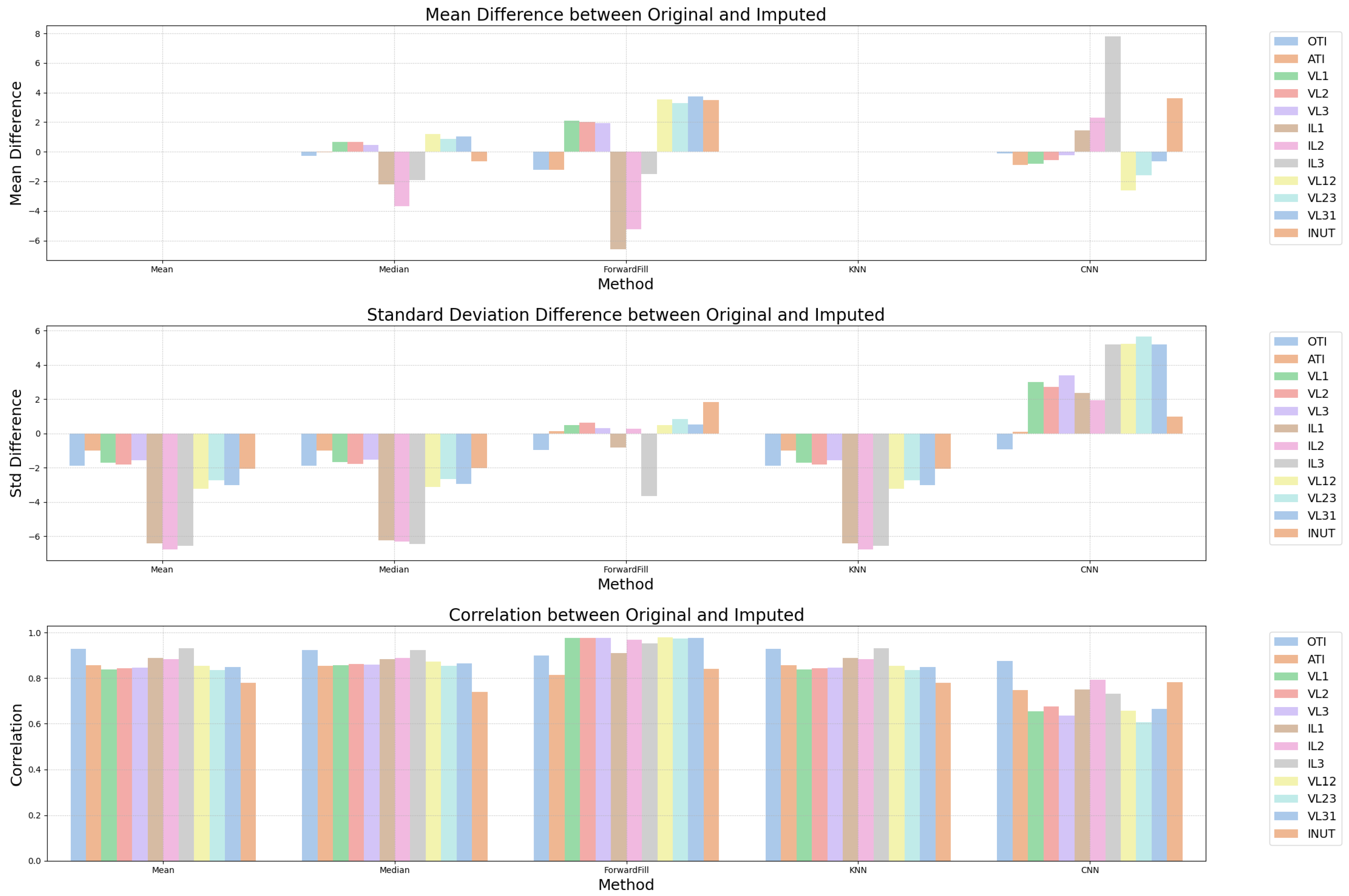
Figure 6 presents a comparative analysis in three parts: (i) the difference between the means before and after imputation, (ii) the difference between the standard deviations, and (iii) the correlation between the original and imputed data. The high correlation coefficients (close to 1.0 for all variables) demonstrate that the imputed values preserve the dynamics of the original signal. Small variations in the means and standard deviations, especially in the current and voltage measurements, reflect the smoothing effect introduced by the model, which contributes to stabilizing the time series without eliminating significant patterns.

4.2. Clustering and Data Analysis in the Frequency Domain

The K-means algorithm was applied to group the numerical data into three clusters, as shown in Figure 7. Next, the Euclidean distance of each point to the centroid of its group was calculated as shown in

Table 4. Power transformer data points by cluster and distance or centroid.

Device Time Stamp	OTI	ATI	VL1	…	IL1	VL12	INUT	Cluster	Distance to Centroid
43,694.46	244.00	33.25	230.88	…	68.85	398.03	14.43	0	217.97
43,694.50	38.75	33.75	229.58	…	31.43	396.15	11.13	1	70.86
43,660.13	0.00	0.00	0.00	…	0.00	0.00	0.00	2	823.23

. The furthest point in each cluster was identified as a potential outlier. The results show the following:

• Cluster 0: Point with high OTI value and high currents.
• Cluster 1: Moderate values, distant but not extreme.
• Cluster 2: Null values in all variables, resulting in the greatest distance proportional to its centroid.

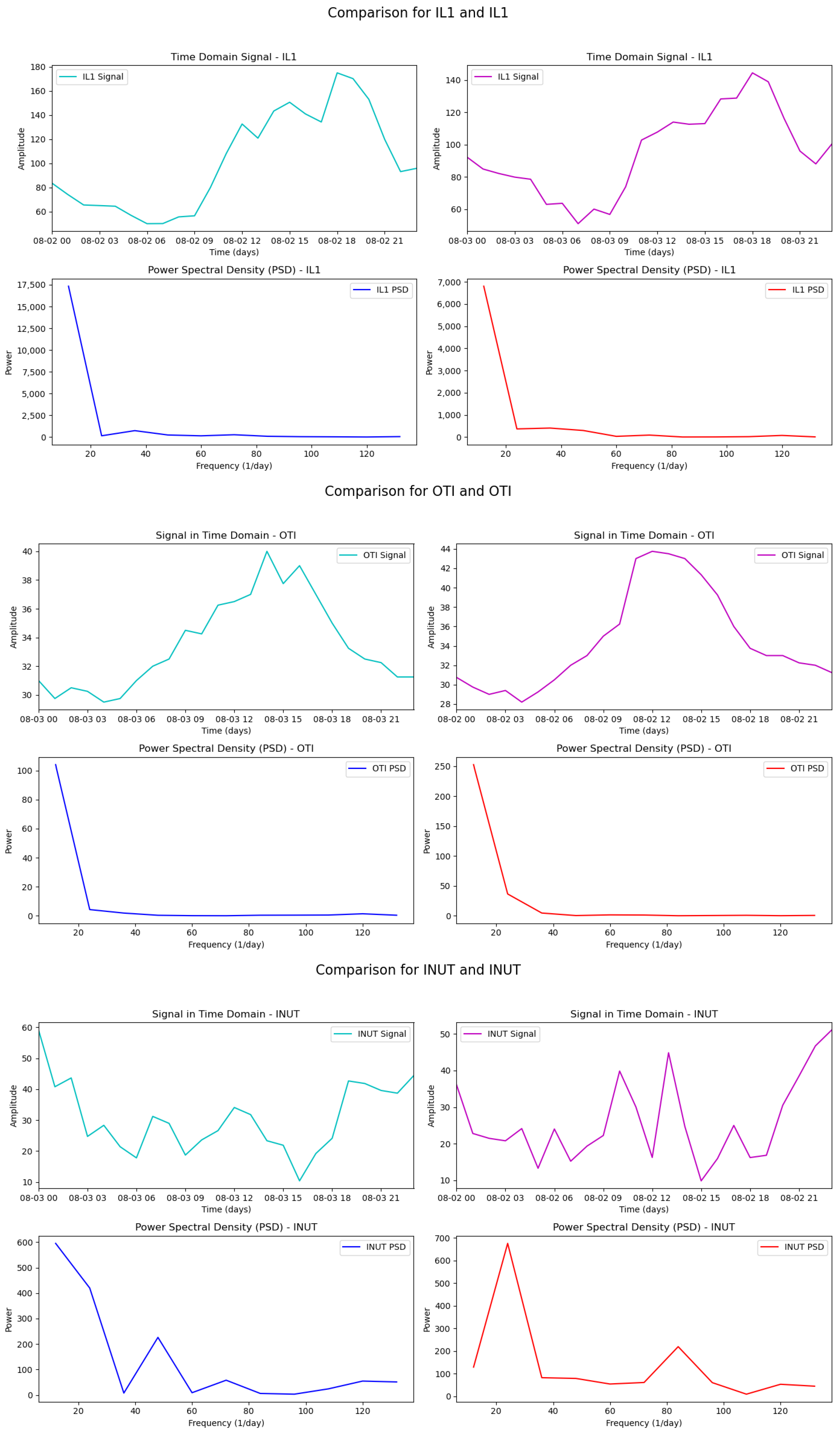
The time-domain analysis in Figure 8 shows that VL2 presents smooth variations (224–240) and a stable cyclical pattern, while INUT exhibits greater irregularity (10–60) and more abrupt oscillations. IL1 presents the highest amplitudes (50–175), with wide variations and a predominance of low frequencies.

In the frequency domain, the PSD of VL2 is strongly concentrated at low frequencies, indicating stable behavior. INUT has multiple peaks, suggesting a mixture of slow and intermediate components. IL1 exhibits much higher power, almost entirely at low frequencies, evidencing large-scale, high-energy events.

4.3. Prediction of Patterns in Power Transformer Data

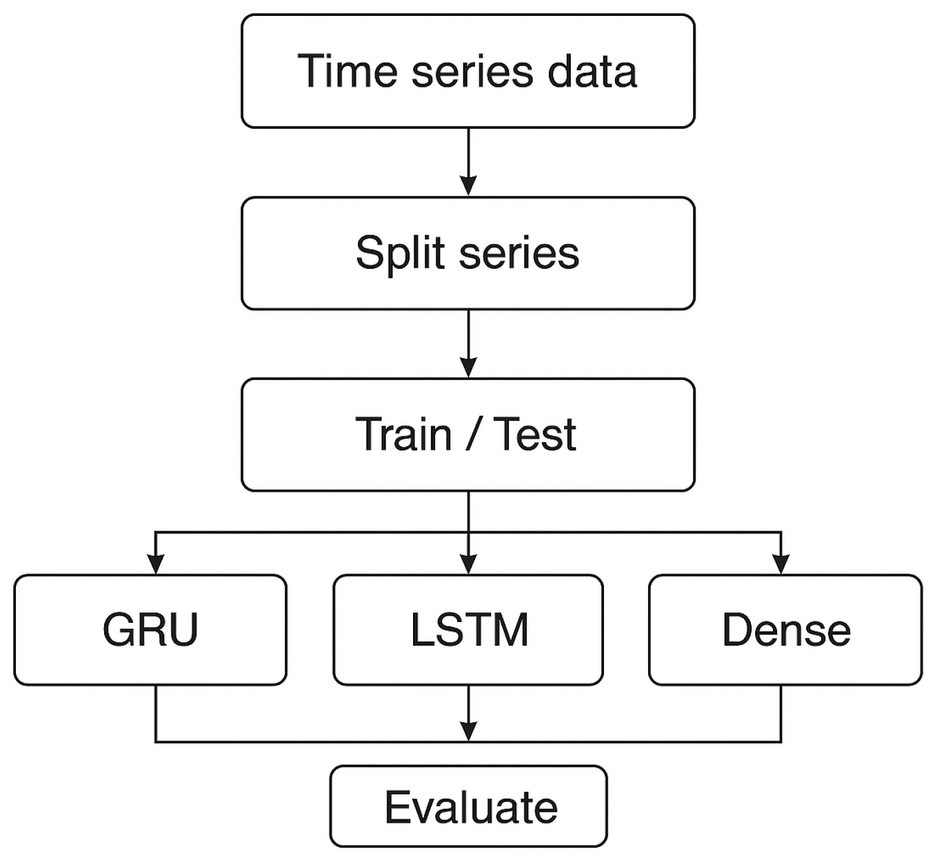
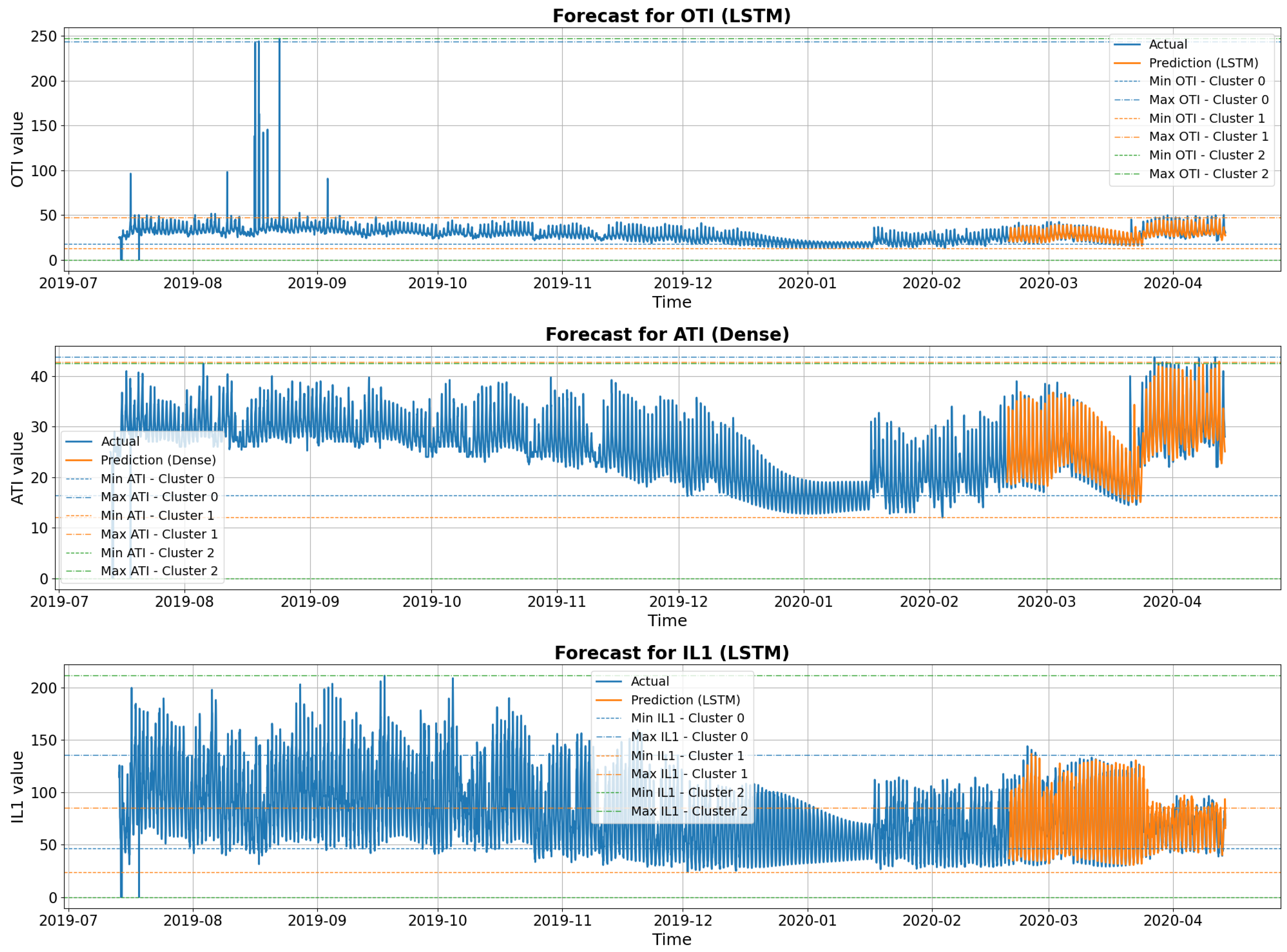
The hourly resolution dataset was organized in the variable df, which included all variables of interest. For data preparation, a sliding window strategy was applied, considering 10 past steps to forecast 20 future steps. The dataset was split preserving temporal order, with 80% of the observations allocated for training and 20% for testing. The experimental design is shown in Figure 9.

Three alternative architectures were implemented: a GRU encoder–decoder with 64 units, an LSTM encoder–decoder, also with 64 units, and a fully connected (Dense) network with 128 hidden units. In the recurrent architectures, the encoder compressed the past sequence into a fixed representation, which was repeated across the forecast horizon and decoded step by step. The Dense model flattened the past sequence and directly mapped it into the forecast horizon. In all cases, outputs were structured as univariate multistep predictions, trained and evaluated independently for each monitored variable. Model selection was performed using the lowest RMSE on the test set, ensuring comparability and robustness in performance evaluation.

Training was conducted for 30 epochs, adopting the Huber loss loss function and the Adam optimizer, with an initial learning rate of $1\times {10}^{-3}$ and a progressive reduction of 10% at each epoch, using the Learning Rate Scheduler strategy.

In the forecast graphs in Figure 9, in addition to the actual time series and the estimates produced by the best selected model (GRU, LSTM, or Dense network, depending on the variable), horizontal lines corresponding to these limits were added. The dashed lines represent the minimum values observed in each cluster, while the dotted lines represent the maximum values.

After the model adjustments, predictions were generated for both the training and test datasets. The performance was quantified for each variable using the metrics mean absolute percentage error (MAPE), root mean square error (RMSE), mean absolute error (MAE), and coefficient of determination ($R^2$).

To complement the quantitative assessment, visual comparisons between the actual and predicted values were performed, allowing a more intuitive analysis of model adherence. The consolidated metric results were summarized in a table and are further discussed in the following section. The comparative evaluation revealed that performance varied depending on the analyzed variable. The LSTM model performed best only for OTI (RMSE = 2.55; $R^2$ = 0.85), whereas the GRU achieved superior results in INUT (RMSE = 6.71; $R^2$ = 0.59). In contrast, the CNN-based model demonstrated overall higher consistency, preserving data dynamics and ensuring robust imputations across variables. Nonetheless, the Dense (MLP) architecture achieved the best numerical accuracy in most cases, particularly for ATI (RMSE = 1.81; $R^2$ = 0.91), and maintained competitive performance in series such as VL1, VL2, and VL31 ($R^2$ ranging from 0.62 to 0.76). Figure 10 presents representative plots illustrating the predictive behavior of the proposed model.

The results, as shown in

Table 5. Performance of prediction models by variable: MAPE, RMSE, MAE, and R² metrics. The best values for each metric are highlighted in bold.

Variable	Best Model	MAPE	RMSE	MAE	R2
OTI	Dense	0.055905	2.678454	1.664657	0.846432
ATI	Dense	0.051844	2.287017	1.364484	0.876268
VL1	Dense	0.007011	2.326546	1.732341	0.745781
VL2	Dense	0.007081	2.590326	1.732341	0.682847
VL3	LSTM	0.011161	3.428184	2.736036	0.454651
IL1	Dense	0.086615	8.875986	6.088209	0.900197
IL2	Dense	0.149841	8.860712	6.012136	0.868971
IL3	Dense	0.096362	11.099322	7.388124	0.892436
VL12	Dense	0.007188	4.140241	3.042514	0.776893
VL23	LSTM	0.007763	4.513046	3.279813	0.673239
VL31	GRU	0.014124	7.268373	5.996321	0.309541
INUT	Dense	0.165428	6.853638	4.934111	0.727558

, for variables such as IL1, IL2, and IL3, show that despite higher RMSE values (8.37–9.25), the coefficients of determination remained high (≈0.88), indicating a good capture of variability. MAPE remained low in almost all series, confirming the relative accuracy of the forecasts.

5. Discussion

The results obtained show that different neural network architectures have complementary performances, highlighting the robustness of the dense architecture (MLP) in several variables and the accuracy of LSTM and GRU in specific cases. This diversity of responses suggests that there is no single model capable of capturing all the dynamics of the transformer, but, rather, there is an ecosystem of techniques that, together, offer greater reliability.

The analysis of critical variables, such as OTI and line currents, confirms that intelligent imputation allows for the reconstruction of time series with high fidelity, enabling subsequent analyses in the time and spectral domains with less risk of bias. This capability is essential for industrial contexts, where sensor failures and data gaps are inevitable.

Another relevant point is the contribution of frequency analysis and clustering to the early identification of anomalous patterns. This approach not only complements time series forecasting but also reinforces the usefulness of hybrid techniques, which cross-reference physical, statistical, and artificial intelligence variables to characterize asset behavior.

This study reinforces the importance of data-driven methodologies in predictive maintenance. The integration of imputation, forecasting, and spectral analysis creates an innovative framework capable of supporting decision making in real industrial environments, with a direct impact on cost reduction, increased reliability, and operational risk mitigation.

6. Conclusions

This study proposed a hybrid framework for imputing and predicting incomplete multivariate time series from real transformers, combining deep learning architectures with temporal, spectral, and clustering analysis. The results showed that LSTM networks achieved the lowest imputation errors in specific cases, while Dense architectures provided more stable performance overall, highlighting their complementary strengths.

By integrating frequency analysis and clustering with imputation and forecasting, the approach revealed hidden patterns and improved failure prediction, demonstrating practical applicability for predictive maintenance in industrial environments. This contribution fills an important gap by addressing data incompleteness with a comprehensive and reliable methodology, supporting cost reduction, improved asset availability, and operational risk mitigation. Future work will focus on extending this framework to real-time monitoring and integration with intelligent maintenance platforms, enhancing responsiveness and decision making in Industry 4.0 contexts.

References

1. Yazdi, M. Maintenance Strategies and Optimization Techniques. In Advances in Computational Mathematics for Industrial System Reliability and Maintainability; Springer Nature: Cham, Switzerland, 2024; pp. 43–58. [Google Scholar] [CrossRef]
2. Sandu, G.; Varganova, O.; Samii, B. Managing physical assets: A systematic review and a sustainable perspective. Int. J. Prod. Res. 2023, 61, 6652–6674. [Google Scholar] [CrossRef]
3. Farinha, J.M.T. Asset Maintenance Engineering Methodologies, 1st ed.; Taylor & Francis Ltd.: Oxfordshire, UK, 2020; p. 336. [Google Scholar]
4. Velmurugan, R.S.; Dhingra, T. Asset Maintenance in Operations-Intensive Organizations. In Asset Maintenance Management in Industry: A Comprehensive Guide to Strategies, Practices and Benchmarking; Springer International Publishing: Cham, Switzerland, 2021; pp. 23–59. [Google Scholar] [CrossRef]
5. Farinha, J.T.; Raposo, H.D.N.; de-Almeida-e Pais, J.E.; Mendes, M. Physical Asset Life Cycle Evaluation Models—A Comparative Analysis towards Sustainability. Sustainability 2023, 15, 15754. [Google Scholar] [CrossRef]
6. Mirshekali, H.; Santos, A.Q.; Shaker, H.R. A Survey of Time-Series Prediction for Digitally Enabled Maintenance of Electrical Grids. Energies 2023, 16, 6332. [Google Scholar] [CrossRef]
7. Balaraman, S.; Kamaraj, N. Cascade BPN based transmission line overload prediction and preventive action by generation rescheduling. Neurocomputing 2012, 94, 1–12. [Google Scholar] [CrossRef]
8. Sharma, S.; Srivastava, L. Prediction of transmission line overloading using intelligent technique. Appl. Soft Comput. 2008, 8, 626–633. [Google Scholar] [CrossRef]
9. Lee, J.; Ni, J.; Singh, J.; Jiang, B.; Azamfar, M.; Feng, J. Intelligent Maintenance Systems and Predictive Manufacturing. J. Manuf. Sci. Eng. 2020, 142, 110805. [Google Scholar] [CrossRef]
10. Sagharidooz, M.; Soltanali, H.; Farinha, J.T.; Raposo, H.D.N.; de-Almeida-e Pais, J.E. Reliability, Availability, and Maintainability Assessment-Based Sustainability-Informed Maintenance Optimization in Power Transmission Networks. Sustainability 2024, 16, 6489. [Google Scholar] [CrossRef]
11. Cachada, A.; Barbosa, J.; Leitño, P.; Gcraldcs, C.A.; Deusdado, L.; Costa, J.; Teixeira, C.; Teixeira, J.; Moreira, A.H.; Moreira, P.M.; et al. Maintenance 4.0: Intelligent and Predictive Maintenance System Architecture. In Proceedings of the 2018 IEEE 23rd International Conference on Emerging Technologies and Factory Automation (ETFA), Torino, Italy, 4–7 September 2018; Volume 1, pp. 139–146. [Google Scholar] [CrossRef]
12. Parpala, R.C.; Iacob, R. Application of IoT concept on predictive maintenance of industrial equipment. MATEC Web Conf. 2017, 121, 02008. [Google Scholar] [CrossRef]
13. Silvestri, L.; Forcina, A.; Introna, V.; Santolamazza, A.; Cesarotti, V. Maintenance transformation through Industry 4.0 technologies: A systematic literature review. Comput. Ind. 2020, 123, 103335. [Google Scholar] [CrossRef]
14. Singh, S.; Galar, D.; Baglee, D.; Björling, S.E. Self-maintenance techniques: A smart approach towards self-maintenance system. Int. J. Syst. Assur. Eng. Manag. 2014, 5, 75–83. [Google Scholar] [CrossRef]
15. Mateus, B.C.; Farinha, J.T.; Mendes, M. Fault Detection and Prediction for Power Transformers Using Fuzzy Logic and Neural Networks. Energies 2024, 17, 296. [Google Scholar] [CrossRef]
16. Martins, A.; Fonseca, I.; Farinha, J.T.; Reis, J.; Cardoso, A.J.M. Prediction maintenance based on vibration analysis and deep learning—A case study of a drying press supported on a Hidden Markov Model. Appl. Soft Comput. 2024, 163, 111885. [Google Scholar] [CrossRef]
17. McKinsey & Company. A Smarter Way to Digitize Maintenance and Reliability. 2021. Available online: https://www.mckinsey.com/capabilities/operations/our-insights/a-smarter-way-to-digitize-maintenance-and-reliability (accessed on 23 May 2025).
18. Crespo Marquez, A.; Gomez Fernandez, J.F.; Martínez-Galán Fernández, P.; Guillen Lopez, A. Maintenance Management through Intelligent Asset Management Platforms (IAMP). Emerging Factors, Key Impact Areas and Data Models. Energies 2020, 13, 3762. [Google Scholar] [CrossRef]
19. Zhang, X.; Li, H.; Wu, P. Data-Driven Construction Safety Information Sharing System Based on Linked Data, Ontologies, and Knowledge Graph Technologies. Int. J. Environ. Res. Public Health 2022, 19, 794. [Google Scholar] [CrossRef]
20. Feng, Y.; Wang, H.; Xia, G.; Cao, W.; Li, T.; Wang, X.; Liu, Z. A machine learning-based data-driven method for risk analysis of marine accidents. J. Mar. Eng. Technol. 2025, 24, 147–158. [Google Scholar] [CrossRef]
21. Dalzochio, J.; Kunst, R.; Pignaton, E.; Binotto, A.P.D.; Sanyal, S.; Favilla, J.; Barbosa, J.L.V. Machine learning and reasoning for predictive maintenance in Industry 4.0: Current status and challenges. Comput. Ind. 2020, 123, 103298. [Google Scholar] [CrossRef]
22. Wan, J.; Tang, S.; Li, D.; Wang, S.; Liu, C.; Abbas, H.; Vasilakos, A.V. A Manufacturing Big Data Solution for Active Preventive Maintenance. IEEE Trans. Ind. Inform. 2017, 13, 2039–2047. [Google Scholar] [CrossRef]
23. Roosefert Mohan, T.; Preetha Roselyn, J.; Annie Uthra, R.; Devaraj, D.; Umachandran, K. Intelligent machine learning based total productive maintenance approach for achieving zero downtime in industrial machinery. Comput. Ind. Eng. 2021, 157, 107267. [Google Scholar] [CrossRef]
24. NP EN 13306:2007; Maintenance Terminology; Portuguese standard based on EN 13306:2007. Instituto Português da. Qualidade: Caparica, Portugal, 2007.
25. Paolanti, M.; Romeo, L.; Felicetti, A.; Mancini, A.; Frontoni, E.; Loncarski, J. Machine Learning approach for Predictive Maintenance in Industry 4.0. In Proceedings of the 2018 14th IEEE/ASME International Conference on Mechatronic and Embedded Systems and Applications (MESA), Oulu, Finland, 2–4 July 2018; pp. 1–6. [Google Scholar] [CrossRef]
26. Malta, A.; Farinha, T.; Mendes, M. Augmented Reality in Maintenance—History and Perspectives. J. Imaging 2023, 9, 142. [Google Scholar] [CrossRef]
27. Compare, M.; Baraldi, P.; Zio, E. Challenges to IoT-Enabled Predictive Maintenance for Industry 4.0. IEEE Internet Things J. 2020, 7, 4585–4597. [Google Scholar] [CrossRef]
28. Javaid, M.; Haleem, A.; Singh, R.P.; Rab, S.; Suman, R. Significance of sensors for industry 4.0: Roles, capabilities, and applications. Sens. Int. 2021, 2, 100110. [Google Scholar] [CrossRef]
29. Mateus, B.; Farinha, J.T.; Cardoso, A.M. Production optimization versus asset availability—A review. WSEAS Trans. Syst. Control 2020, 15, 320–332. [Google Scholar] [CrossRef]
30. Elnahrawy, E.; Nath, B. Cleaning and querying noisy sensors. In Proceedings of the 2nd ACM International Conference on Wireless Sensor Networks and Applications, San Diego, CA, USA, 19 September 2003; WSNA ’03. Association for Computing Machinery: New York, NY, USA, 2003; pp. 78–87. [Google Scholar] [CrossRef]
31. McGrath, M.J.; Scanaill, C.N. Sensing and Sensor Fundamentals. In Sensor Technologies: Healthcare, Wellness, and Environmental Applications; Apress: Berkeley, CA, USA, 2013; pp. 15–50. [Google Scholar] [CrossRef]
32. Fraden, J. Sensor Characteristics. In Handbook of Modern Sensors: Physics, Designs, and Applications; Springer: New York, NY, USA, 2010; pp. 13–52. [Google Scholar] [CrossRef]
33. North, D. An Analysis of the factors which determine signal/noise discrimination in pulsed-carrier systems. Proc. IEEE 1963, 51, 1016–1027. [Google Scholar] [CrossRef]
34. Shuai, M.; Xie, K.; Chen, G.; Ma, X.; Song, G. A Kalman Filter Based Approach for Outlier Detection in Sensor Networks. In Proceedings of the 2008 International Conference on Computer Science and Software Engineering, Wuhan, China, 12–14 December 2008; Volume 4, pp. 154–157. [Google Scholar] [CrossRef]
35. Tan, Y.L.; Sehgal, V.; Shahri, H.H. Sensoclean: Handling Noisy and Incomplete Data in Sensor Networks Using Modeling. Ph.D. Thesis, University of Kaiserslautern, Kaiserslautern, Germany, 2005; pp. 1–18. [Google Scholar]
36. Shao, B.; Song, C.; Wang, Z.; Li, Z.; Yu, S.; Zeng, P. Data Cleaning Based on Multi-sensor Spatiotemporal Correlation. In Machine Learning and Intelligent Communications; Zhai, X.B., Chen, B., Zhu, K., Eds.; Springer International Publishing: Cham, Switzerland, 2019; pp. 235–243. [Google Scholar]
37. Liu, H.; Shah, S.; Jiang, W. On-line outlier detection and data cleaning. Comput. Chem. Eng. 2004, 28, 1635–1647. [Google Scholar] [CrossRef]
38. Hyndman, R.J.; Athanasopoulos, G. Forecasting: Principles and Practice, 3rd ed.; OTexts: Munich, Germany, 2021. [Google Scholar]
39. Keogh, E.; Kasetty, S. On the need for time series data mining benchmarks: A survey and empirical demonstration. In Proceedings of the Ninth ACM SIGKDD International Conference on Knowledge Discovery and Data Mining, ACM, Washington, DC, USA, 24–27 August 2003; pp. 102–111. [Google Scholar]
40. Esling, P.; Agon, C. Time-series data mining. ACM Comput. Surv. (CSUR) 2012, 45, 1–34. [Google Scholar] [CrossRef]
41. Yoon, J.; Jarrett, D.; van der Schaar, M. Semi-supervised learning with deep generative models for high-dimensional missing data imputation. Adv. Neural Inf. Process. Syst. (NeurIPS) 2020, 33, 8050–8060. [Google Scholar]
42. Zhang, Z.; Chen, J.; Yu, T.; Wang, Z. Missing value imputation for microarray gene expression data using a weighted KNN algorithm with truncated normal distribution. BMC Bioinform. 2017, 18, 1–12. [Google Scholar]
43. Dempster, A.P.; Laird, N.M.; Rubin, D.B. Maximum Likelihood from Incomplete Data via the EM Algorithm. J. R. Stat. Soc. Ser. B (Methodol.) 1977, 39, 1–38. [Google Scholar] [CrossRef]
44. Schmitt, M.; Zhu, X.X. Missing Data Imputation for Remote Sensing Time Series by Out-of-Sample EM. In Machine Learning and Knowledge Discovery in Databases; Springer: Berlin/Heidelberg, Germany, 2019; pp. 347–363. [Google Scholar] [CrossRef]
45. Wu, Z.; Li, Z.; Liu, Q. Semi-supervised learning with missing not at random data. arXiv 2023. Available online: https://arxiv.org/abs/2308.08872 (accessed on 1 June 2025).
46. Abdalla, H.I.; Altaf, A. The Impact of Data Normalization on KNN Rendering. In Proceedings of the 9th International Conference on Advanced Intelligent Systems and Informatics, Cairo, Egypt, 20–22 September 2023; Hassanien, A., Rizk, R.Y., Pamucar, D., Darwish, A., Chang, K.C., Eds.; Springer Nature: Cham, Switzerland, 2023; pp. 176–184. [Google Scholar]
47. Pagan, M.; Zarlis, M.; Candra, A. Investigating the impact of data scaling on the k-nearest neighbor algorithm. Comput. Sci. Inf. Technol. 2023, 4, 135–142. [Google Scholar] [CrossRef]
48. Henderi, H.; Wahyuningsih, T.; Rahwanto, E. Comparison of Min-Max normalization and Z-Score Normalization in the K-nearest neighbor (kNN) Algorithm to Test the Accuracy of Types of Breast Cancer. Int. J. Inform. Inf. Syst. 2021, 4, 13–20. [Google Scholar] [CrossRef]
49. Ahmed, H.A.; Ali, P.J.M.; Faeq, A.K.; Abdullah, S.M. An investigation on disparity responds of machine learning algorithms to data normalization method. Aro-Sci. J. Koya Univ. 2022, 10, 29–37. [Google Scholar] [CrossRef]
50. Abid, A.; Khan, M.T.; Iqbal, J. A review on fault detection and diagnosis techniques: Basics and beyond. Artif. Intell. Rev. 2021, 54, 3639–3664. [Google Scholar] [CrossRef]
51. Brito, L.; Susto, G.; Brito, J.; Duarte, M. An explainable artificial intelligence approach for fault detection. Signal Process. Syst. 2022. [Google Scholar] [CrossRef]
52. Shakiba, F.; Azizi, S.; Zhou, M.; Abusorrah, A. Application of machine learning methods in fault detection. Artif. Intell. Rev. 2023. [Google Scholar] [CrossRef]
53. Azamfar, M.; Singh, J.; Bravo-Imaz, I.; Lee, J. Multisensor data fusion for gearbox fault diagnosis. Signal Process. Syst. 2020. [Google Scholar] [CrossRef]
54. Kiranyaz, S.; Ince, T.; Abdeljaber, O.; Avci, O.; Gabbouj, M. 1-D convolutional neural networks for signal processing applications. IEEE Trans. Signal Process. 2019. [Google Scholar]
55. Chen, Y.; Rao, M.; Feng, K.; Zuo, M. Physics-Informed LSTM hyperparameters selection for fault detection. Signal Process. Syst. 2022. [Google Scholar] [CrossRef]
56. Ali, M.; Shabbir, M.; Liang, X.; et al. Machine learning-based fault diagnosis for synchronous motors. IEEE Trans. 2019. [Google Scholar]
57. Kumar, P.; Hati, A. Review on machine learning algorithms for fault detection. Arch. Comput. Methods Eng. 2021. [Google Scholar] [CrossRef]
58. Yu, J.; Zhang, Y. Challenges and opportunities of deep learning-based predictive maintenance. Neural Comput. Appl. 2023. [Google Scholar] [CrossRef]
59. Samanta, A.; Chowdhuri, S.; Williamson, S. Machine learning-based fault detection in electric vehicles. Electronics 2021. [Google Scholar]
60. Kingma, D.P.; Ba, J. Adam: A method for stochastic optimization. arXiv 2014, arXiv:1412.6980. [Google Scholar]
61. Javaid, M.; Khan, M.; Lee, J. Signal processing techniques for condition monitoring of electrical machines. IEEE Access 2021, 9, 12034–12050. [Google Scholar]
Figure 1. Bibliometric analysis using the keywords “fault detection” AND “machine learning” AND “signal processing”.
Energies 18 05634 g001
Figure 2. Encoder–decoder architecture with deep neural networks for data imputation and prediction.
Energies 18 05634 g002
Figure 3. Time series of each transformer variable, with a sampling rate of 15 min.
Energies 18 05634 g003
Figure 4. Time series of each transformer variable, with a sampling rate of 1 h.
Energies 18 05634 g004
Figure 5. Increased data in the time series using different approaches.
Energies 18 05634 g005
Figure 6. Comparison of statistical metrics before and after imputation.
Energies 18 05634 g006
Figure 7. Frequency-domain behavior clustering using K-means.
Energies 18 05634 g007
Figure 8. Comparison of transformer signals in time and frequency domains.
Energies 18 05634 g008
Figure 9. Study architecture structure.
Energies 18 05634 g009
Figure 10. Temporary series with data incrementation.
Energies 18 05634 g010