Abstract
Recent years have seen a considerable increase in clean, green electricity output from wind energy (WE). It is crucial to obtain the optimum parameters of the two-parameter Weibull distribution (TPWD) for wind speed (WS) to calculate the potential WE. This paper proposes to use the superEGO (SEGO) along with maximum likelihood estimation (MLE) to obtain optimum parameters of the TWPD for WS data. The results showed that SEGO provided better results compared other optimization algorithms used in this context. Moreover, the potential WE for Gdańsk, a city located by the Baltic Sea in northern Poland, was calculated using parameters obtained by using SEGO. It was observed that SEGO performs the best among other optimization algorithms to find optimum parameters for the two-parameter Weibull distribution along with MLE for wind speed.
1. Introduction
Energy is an important factor in the advancement of civilization, as every economic process requires an energy supply. Nonetheless, its impact on society and the economy has never been greater. Modern society, individual homes, and the economy cannot run without reliable energy sources. However, using fossil fuels during manufacturing is one of the most important drivers of air pollution, especially the release of greenhouse gases and carbon dioxide [1]. In the absence of significant measures, climate change will intensify, particularly affecting Africa and India. As a result, there will be an increase in the number of people migrating to different places, including Poland and Europe (also known as climate movement) [2].
Renewable energy sources (RESs) are referred to as natural resources that generate energy through processes and are constantly replenished by the International Energy Agency (IEA). These include solar energy, wind, hydropower, biomass, geothermal energy, and tidal power [3]. Solar energy, for instance, is derived from the sun’s rays. With the improved technology of solar panels, nowadays, it is even possible to generate electricity using solar energy during cloudy days [4]. WE is produced by the movement of air. Even though every location in the world has a different WE capacity, the existing global potential WE exceeds today’s global energy production. Hydropower depends on the water cycle. Although hydropower provides sustainable and green energy, it is very much impacted by climate change (e.g., due to global warming leading to less and less rain). Biomass energy is produced by burning organic waste in simple words. However, during biomass energy production, gas emission occurs. Even though this gas emission is lower than that produced by fossil fuels, it is important to carefully plan the usage of biomass energy. While tidal power draws on the moon’s gravitational pull, geothermal energy draws on heat from below the Earth’s surface. The technology used for geothermal energy is fairly well-developed and has been used for over a century. Unlike fossil fuels, which are finite and harmful to the environment, renewable sources are virtually endless and produce less pollution. They are key to combating climate change, boosting energy security, and creating new jobs and technologies. As renewable energy costs continue to drop, it is becoming an increasingly practical and affordable option for communities around the world [5,6,7].
The EU Green Deal aims to neutralize greenhouse gas emissions and transform the economy by 2050 [8]. This document guides EU Member State policy on energy efficiency, climate change, and sustainable development [9,10].
The invasion of Ukraine by Russia brought about a change in the circumstances surrounding energy policy. The conflict highlighted energy independence, renewable energy, and greenhouse gas reduction. In response, the European Commission announced the REPowerEU Action Plan [11] to accelerate investments in renewable energy sources and renewable hydrogen infrastructure to minimize greenhouse gas emissions and the EU’s dependency on Russian fossil fuel imports. This would raise the EU’s binding renewable energy objective from 40% in Fit-for-55 to 42.5%.
The report “Poland’s Energy Policy until 2040”, which was adopted at the end of March 2022, highlights strengthening the country’s energy security and independence. In relation to renewable energy sources, their further development and an increase in their role in the diversification of the electricity mix were announced. According to the report, the goal is to increase the share of renewable energy sources in electricity production to 50%. The need for financial support to achieve energy self-sufficiency for individual households is also foreseen. One of the government’s priorities is to increase the potential for storing electricity and heat at the level of prosumers, renewable energy producers, network operators, and aggregators [12].
Wind turbines, a component of wind power plants, are a very straightforward technical solution for harnessing WE. These plants transform the mechanical or electrical energy contained in the wind’s kinetic energy. Power stations, either standalone or part of larger clusters known as wind parks or farms, are the primary sources of electricity generation [13].
In 2023, the global WE sector increased their capacity by 117 GW, comprising 106.1 GW from onshore installations and 10.9 GW from offshore projects. WE capacity has risen 12.8% year-on-year [7,10]. China dominates the global wind power market, accounting for two-thirds of the newly installed capacity worldwide. China has also broken records for investments in offshore projects and turbine orders, the latter of which will be deployed in 2024. In 2023, wind power accounted for at least 25% of electricity production in several nations, including eight European nations and Uruguay. The “wind” map now includes three more countries: Djibouti, Mauritania, and the UAE [8].
Wind power is projected to expand further in the coming years, as it remains one of the most cost-effective energy sources, driving economic growth, job creation, and enhanced energy security. Over 130 countries aim to triple their renewable energy capacity—primarily solar and wind—by 2030 to cut greenhouse gas emissions and mitigate climate change [14].
The main objective of this paper is to propose a novel approach for obtaining parameters for the two-parameter Weibull distribution (TPWD) for wind speed using SEGO along with MLE.
In pursuit of this objective, the authors provided the subsequent additional contributions. An overview of WE development in Poland, specifically focusing on the Pomeranian Voivodeship, a region identified as having significant WE potential, was provided. A new method for estimating the parameters of the Weibull distribution for WS was introduced to enhance the efficiency of estimating the potential WE. Hourly weather data for Gdańsk, Poland, spanning seven years, was used in this study. SEGO was used along with MLE to fit the two-parameter Weibull distribution (TPWD) to WS and determine the optimum TPWD parameters as a novel approach. Furthermore, the performance of SEGO was compared to the Genetic Algorithm (GA), the Simulated Annealing (SA), Differential Evolution (DE), and Efficient Global Optimization (EGO), which are methods in the literature used to find the optimum parameters of the TPWD for WS along with MLE. In particular, Aydin et al. used EGO to obtain the parameters of the TPWD for wind speed data. They compared the performance of EGO with the GA, the SA, and DE. The coefficient of determination (R2) and root mean-squared error (RMSE) showed that EGO performs better compared to the others. In this study, the SEGO algorithm is proposed and compared with other methods. Using each method, parameters were estimated for each month and on whole data; R2 and RMSE were used to compare the performance of these five different methods [15,16,17]. SEGO is a modified version of EGO that utilizes the DIRECT algorithm. This allows it to perform better to find optimum values. The analysis showed that SEGO performed better for finding the optimum parameters of the TPWD for wind speed. Using these parameters, the potential WE for Gdańsk city center was calculated under the assumption of having a wind turbine designed for urban environments at a certain height.
2. Advancements in Poland’s Wind Energy Market
2.1. Wind Energy in Poland
Since the early 1990s, Poland has been actively investing in WE as a key component of renewable energy by recognizing the potential of it to reduce dependency on fossil fuels. Over the years, increased investment in both onshore and offshore wind farms have contributed to expanding WE capacity in the country. Today, WE plays a crucial role in Poland’s strategy regarding the transition to the usage of more sustainable and environmentally friendly energy, which aligns with the European Union’s regulations and climate act. In 1991, Poland’s first modern wind turbine was installed at the Hydroelectric Power Plant in Żarnowiec. The country’s first industrial wind farm was the Barzowice wind farm in the West Pomeranian Voivodeship, which opened in April 2001. The system comprised six power plants, with a 5 MW capacity collectively [18].
Onshore WE has lost its leading position in the renewable energy sector since 2021 due to PV prosumers, but it is still growing dynamically. At the end of 2024 in Poland, the installed onshore wind capacity was 9.43 GW, and this should soon exceed the 10 GW threshold. For comparison, the installed capacity for the entire national power system was 66.4 GW (conventional energy and RE), so the share of onshore wind farms was 14% of the total capacity [18].
Polish Energy Policy indicates that the anticipated capacity of wind turbines is projected to reach 14 GW by 2030 [18].
2.2. Wind Energy in the Pomeranian Voivodeship
The Pomeranian Voivodeship has a total WE capacity of over 1000 MW [18]. Figure 1 represents a map of wind farms. As can be seen in Figure 1, the majority of them are in the northern and eastern parts of the voivodeship.
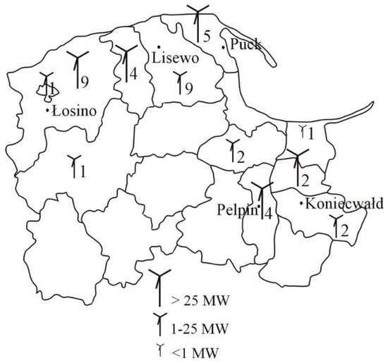
Figure 1.
Wind farm map for Pomeranian Voivodeship (own elaboration based on [5]).
3. Methodology
With advancements in technology, nowadays, it is possible to produce electricity using WE efficiently and cost-effectively. To be able to benefit from WE efficiently, it is crucial to calculate potential WE with high precision. In order to calculate WE with high precision, WS data must be fit to the appropriate statistical distribution and the optimum parameters of the distribution have to be estimated correctly. When calculating potential WE, the TPWD is often used because it provides an efficient way to describe how wind speeds vary over time. This distribution is defined by two key parameters: the shape (k), which shows how wind speeds are spread out, and the scale factor (c), which represents the typical wind speed for a site. These values are usually calculated from historical wind data using statistical methods such as MLE. By using this approach instead of just relying on average wind speed, one can make much more accurate estimates of energy production and choose the best locations for wind turbines.
This study’s scope included gathering WS data for Gdańsk from a third-party vendor for the past seven years. Next, SEGO was used to estimate the optimum parameters of the TPWD through MLE. Finally, the obtained TPWD parameters were used to calculate the potential WE for Gdańsk, a city located in northern Poland.
3.1. Fitting the Statistical Distribution for WS
Since WS is stochastic, it is important to understand and investigate its statistical distribution. Understanding the statistical distribution of WS has a big impact on calculating the potential WE correctly in a given location [19]. The probability distribution function (PDF) shows the statistical characteristics of a random variable. Various PDFs, including Weibull, lognormal, gamma, Rayleigh, and mixed distributions, are used to explain and understand the statistical distribution of WS [20,21,22]. The use of the TPWD for WS is extensively discussed in the literature. The TPWD has two parameters: shape and scale. A comprehensive statistical analysis of these two parameters is essential for the accurate prediction of WE potential and the understanding of WS’s statistical characteristics [20,23,24]. Over the years, researchers have come up with a lot of different ways to find the optimum parameters for the Weibull distribution (WD). The most common methods are the moments method (MOM), the graphics method (GM), the least-squares estimation (LSE), and the maximum likelihood estimation (MLE).
The power density factor and the energy pattern factor were introduced by Akdag and Dinler for WD parameter estimation. These new methods were used for analyzing WE potential for several places in Turkey [23]. Stevens et al. [25] proposed the use of the mean and standard deviation of WS and MLE to find the optimum parameters for WS. Graphical methods and a proposed method called the approximated method were used and compared to estimate WD parameters by Jowder [26]. A study focused on the comparison of empirical methods with graphics methods for estimating the parameters of the WD [27]. In order to estimate TPWD’s shape and size parameters, George compared five different methods [27]. As a conclusion, the MLE provided the best results. Chang ran a comparison for six different numerical methods to estimate the WD’s parameters: GM, MOM, EM, MLE, modified MLE (MMLE), and the energy pattern factor/power density method (EPFPDM). As part of their evaluation for estimating the parameters of the WD, Chang utilized the equivalent energy approach in addition to the six methods that they had previously investigated. Their research indicates that the accuracy of parameter estimation for the WD is correlated with sample size [28]. A metaheuristic optimization technique is another option that can be utilized in addition to numerical methods for the purpose of parameter estimation. In order to predict the parameters of the WD, Chang utilized particle swarm optimization (PSO). This method was then applied on data collected from weather stations located in Taiwan’s several different climate zones. [29]. Rocha et al. compared seven numerical methods for estimating the parameters of the TPWD, using wind speed data collected from the cities of Camocim and Paracuru, State of Ceará, Brazil [30]. Arslan et al. compared the performance of MLE, the Moment Method (MM), and the L-Moment Method (LMM) for estimating the parameters of the TPWD [31]. Usta used probability-weighted moments based on the power density method (PWMBP) to estimate the parameters of the TPWD [32].
Logistic distributions with MLE were used to analyze Inner Mongolia’s potential WE [33]. A new approach to obtain the TPWD parameters with multi-objective moments was proposed by Usta et al. [34]. Tosunoglu et al. compared different methods, including the Method of Moments (MOM), MLE, and Probability-Weighted Moments (PWMs), on different statistical distributions for WS data collected in Türkiye [35]. The TPWD parameters were estimated for analyzing potential wind power in southern India by using nine different computational techniques [15]. Seo et al. used the MLE method for wind turbine power curve modeling [36]. Alrashidi et al. proposed a new method called Social Spider Optimization (SSO) to predict the parameters of the TPWD [37]. Four different numerical approaches were evaluated in terms of their performances to estimate the parameters of the TPWD for Izmir, Türkiye [17]. Kumar et al. used the DE algorithm along with MLE to be able to estimate the TPWD parameters for WS data [38]. Gokcek et al. fit wind data to the WD and Rayleigh distribution in order to investigate the WE potential in Kirklareli, Türkiye [39]. Saxena et al. used the GM and MMLE to estimate wind power density in the Western Rajasthan region in India [40]. To find the most optimum TPWD parameters for calculating Gdansk’s potential WE potential, Aydin et al. used EGO through MLE [41].
When it comes to evaluating the WE potential and statistical distribution of WS, the literature suggests that the TPWD is the most used statistical distribution, and the parameters of the TPWD have been estimated using a variety of optimization algorithms along with MLE. This research study focuses on proposing the use of SEGO with MLE to find the optimum shape and scale parameters of the TPWD.
3.2. Parameter Estimation for the WD Using MLE
Estimation is a technique that is applicable across numerous disciplines, including statistics, economics, engineering design, and others. Estimating the parameters of a statistical distribution is often necessary using a dataset collected through experiments or observations. The literature shows that the most common estimation techniques are MLE, MOM, and GM. However, among these three, MLE is the most frequently preferred one.
MLE is used to determine a set of parameters that maximize the likelihood function. As the literature suggests, WS data typically fits the TPWD. The distribution function of the TPWD is presented in Equation (1), where is the scale and k is the shape parameter of the TPWD and x is an observed value [38,41].
The likelihood function of the TPWD is as follows, where is the scale and k is the shape parameter of the TPWD and x is an observed value:
and the log-likelihood function is shown below, where is the scale and k is the shape parameter of the TPWD and x is an observed value:
3.3. SEGO Algorithm
SEGO was designed for problems where it takes a long time to compute the objective and/or constraint functions by Sasena et al. It fixes these issues by using a Kriging model to obtain a global estimate for each response. As a result of the way the estimates work, SEGO is most suitable for problems with few design variables and few expensive constraints (less than 10). The SEGO algorithm uses Infill Sampling Criteria (ISC), that are obtained using the Expected Improvement approach (EI) [42,43].
Kriging metamodeling is closely linked to SEGO, which is a modified version of EGO. Using an efficient stopping rule based on the EI, EGO requires a low number of evaluations for global optimization problems. The creation of the EI function relies on the Kriging model. Kriging is a mathematical interpolation technique named after mining engineer Krige. He addressed the issue of interpolating findings gained from a restricted number of places in gold mining. Then it has been improved over the years and has become a solid metamodeling technique for many different disciplines.
The Kriging model, in a simple manner, can be formulated as follows:
where and is the mean value, and is the independent error term, which is normally distributed with a zero mean and variance [41,44].
Maximizing the EI function generates a new sampling point. After that, the original set obtains this new data point. This cycle continues until the EI function value remains essentially unchanged. We denote that , where is the minimum response value of . Then the improvement (I) over can be shown as follows:
Under the assumption that y has a normal distribution with a mean equal to and variance equal to , the expected value of I, in other words, the Expected Improvement (EI), is shown in Equations (6) and (7).
where is the cumulative distribution function (CDF) and is the PDF of a standard normal distribution [41,44].
The SEGO starts by taking a small sample of the design domain. Then, it creates a Kriging metamodel. The following step is the optimization of ISC by using an optimization technique called DIRECT. The Kriging metamodel is updated with the new point predicted in each iteration. Continual enhancements to the Kriging metamodels in each iteration facilitate rapid convergence, thereby increasing their accuracy as showed in Figure 2. The global, derivative-free DIRECT algorithm normalizes the feasible region into a unit hyperrectangle and partitions it into smaller hyperrectangles. To solve problems with more than one dimension, the DIRECT method basically evaluates the objective function at the centers of the hyperrectangles. Then it finds and splits the hyperrectangles that have the highest probability of obtaining the lowest objective function value in each iteration based on the Lipschitzian optimization theory [42].
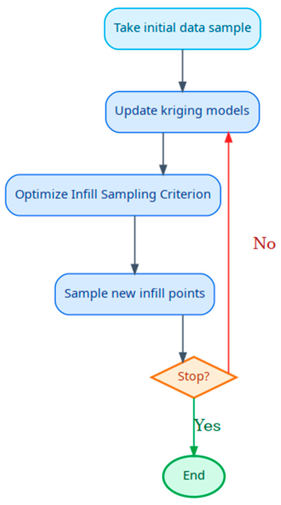
Figure 2.
Flowchart of SEGO (own elaboration based on [43]).
4. Results
A dataset containing hourly WS observations for Gdańsk (latitude: 54.352° N, longitude: 18.646° E, 10 m height) was obtained from the Open Weather Map for the period spanning 1 January 2015 to 26 July 2021 [45]. Then parameters of the TPWD were estimated for WS data on monthly and the whole data separately. With the intention of estimating the parameters of the TPWD, the GA, DE, the SA, EGO and SEGO were used, and a detailed evaluation for each method was provided. Using SEGO, the predicted TPWD parameters were used to evaluate the potential WE and electricity output for Gdańsk.
Table 1 highlights the monthly summary statistics of the dataset, which has 56,880 observations. The table indicates that August is the warmest month in Gdańsk, while January is the coldest. Table 1 additionally displays the average wind speed (m/s) for each month in Gdańsk. The table indicates that April, December, and May are the months with the stronger wind observed, whereas August is the month with the least wind.

Table 1.
Summary statistics.
To determine the optimal TPWD parameters for the WS data, this study utilized thelatest available open source R packages “DiceOptim” for EGO, “DEoptim” for DE, “GA” for the GA, and “optimization” for the SA using R version 4.4.2 [46,47,48,49]. The SEGO MATLAB extension version 4.1 open sourced by Sasena was used for SEGO on MATLAB R2021b [43]. As shown in Table 2, there are not huge differences between the shape (k) and scale (c) parameters estimations obtained by different methods.
Table 2.
Shape (k) and scale (c) parameter estimations on monthly data.
The histogram of WS observations and the estimated PDF curve based on the TPWD for the five techniques for each month of the year are depicted in Figure 3 and Figure 4. The efficacy of the techniques is illustrated in Table 3 and Figure 5 and Figure 6, which are based on two distinct metrics, RMSE and R2, shown in Equations (8) and (9), respectively, where is the observed value, is the predicted value, and is the mean value of observed values. These two metrics are common metrics in statistics used to measure the prediction error. In the literature regarding predicting TPWD parameters, these metrics are also commonly used.
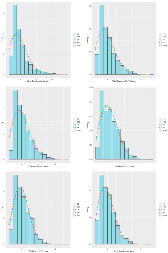
Figure 3.
TPWD fit per month using different techniques (from January to June) (own elaboration).
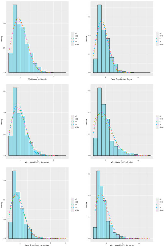
Figure 4.
TPWD fit per month using different techniques (from July to December) (own elaboration).
Table 3.
Performance comparison for different methods.
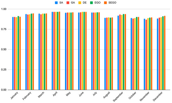
Figure 5.
R-square value per month (own elaboration).
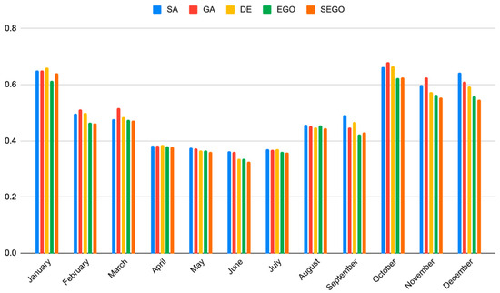
Figure 6.
RMSE value for each technique and for each month (own elaboration).
The RMSE seems to be lower mid-year and higher towards the end of the year. The highest R2 values are observed mid-year. DE and EGO also perform well, especially for mid-year months. However, SEGO outperforms other methods in most cases for the estimation of TPWD parameters, achieving the lowest RMSE and highest R2 values, as evidenced by Table 3 and Figure 5 and Figure 6. The R2 for TPWD parameter estimations for SEGO is higher than for the other techniques for the most months. The RMSE was calculated for estimations based on SEGO is lower than for the other methods.
Table 4 presents the shape (k) and scale (c) parameter estimations on the whole data. The histogram for the WS data and the PDF curve for the TPWD fitted to the WS data using five different methods for the whole data are shown on Figure 7.
Table 4.
Performance comparison and parameter estimation on whole data.
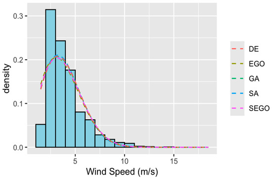
Figure 7.
Distribution fit for each technique on whole data (own elaboration).
The effectiveness of techniques is additionally shown in Table 4, which is based on the two separate metrics: R2 and RMSE.
The lowest RMSE and the maximum R2 are provided by SEGO, as indicated by Table 4 and Figure 8 and Figure 9. In other words, SEGO performs better than all the other techniques in terms of estimating the shape (k) and scale (c) parameters of the TPWD.
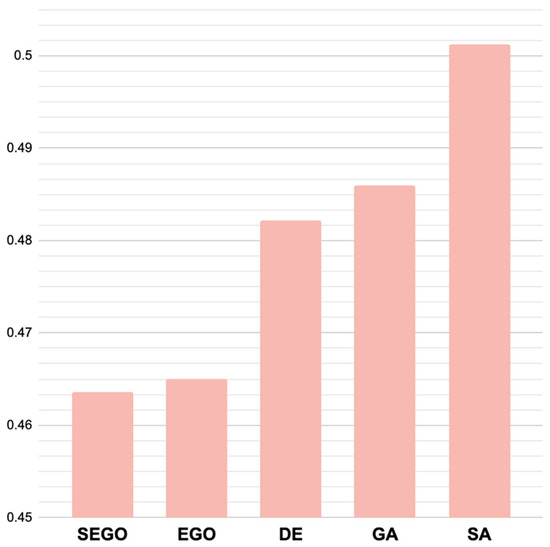
Figure 8.
RMSE for whole data (own elaboration).
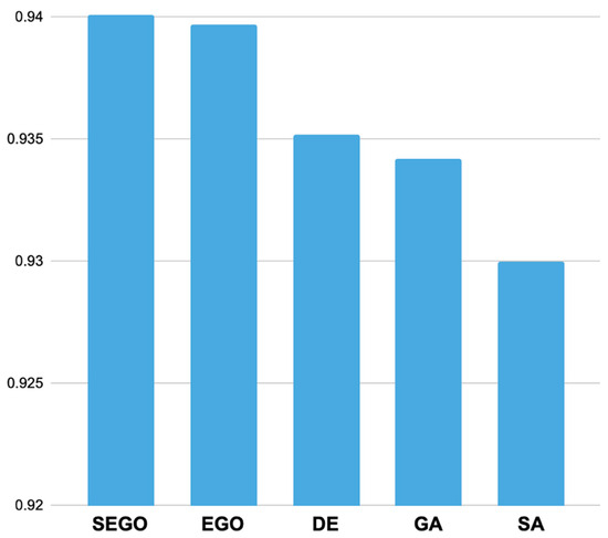
Figure 9.
R2 for whole data (own elaboration).
When the TPWD is used as the PDF of the WS data, the average wind power density per square meter can be calculated using Equation (10), where c is the scale and k is the shape parameter of the TPWD, and is the standard air density, which is assumed to be 1.225 kg/m3 [39,50].
k is estimated as 2.08, and c is estimated as 4.31. Then the wind power density is calculated as 90.47 W/m2.
The Small Wind Guide Book from the U.S. Department of Energy, Office of Energy Efficiency and Renewable Energy, identifies the Skystream 3.7 as a wind turbine well-suited for urban environments. Designed for residential and small commercial applications, the Skystream 3.7 is a grid-connected turbine that operates efficiently even in moderate wind conditions. It has a rated capacity of 1.8 kW and features an advanced inverter that enables its seamless integration into existing electrical systems. According to performance assessments, the Skystream 3.7 can supply between 40% and 90% of the total energy demand of households and small enterprises, depending on local wind resources and energy consumption patterns. Its relatively low noise levels and compact design make it particularly suitable for urban and suburban settings, where space and noise restrictions often limit the feasibility of larger wind turbines [51]. Widespread adoption of small wind turbines like the Skystream 3.7 can contribute to decentralized renewable energy generation, reducing reliance on traditional power grids and lowering carbon emissions. However, the effectiveness of such systems depends on various factors, including local wind speed, zoning regulations, and installation height, which must be carefully evaluated to maximize performance and economic viability. Considering this information, the potential WE is computed based on the setup of a Skystream 3.7 wind turbine in the old town of Gdańsk.
To calculate the potential wind power produced () by the wind turbine mentioned, it is essential to know the swept area (A) and power coefficient () of the wind turbine [52].
The SWA and maximum PC of the Skystream 3.7 are 10.87 m2 and 0.4, respectively [51]. is calculated as 393.3918 W. In order to calculate the potential energy generated annually, , the following formula can be used. in Equation (10) is given in hours [53]. Since in a year there are 8760 h, the yearly average energy that could be produced using the wind turbine is calculated as 3446.112 kWh
To have a precise evaluation of potential WE, seasonal weather conditions and cut-in/cut-out wind speeds for the given wind turbine should be taken into consideration. These assumptions were not considered in this research study.
5. Conclusions and Recommendations
This article presents an analysis of potential WE, which is an important and topical issue related to the global energy transition [54]. Among the many forms of renewable energy, wind power is among the fastest growing. When it comes to the development of renewable energy technology, including WE, attention should be paid to the issue of preparing adequate financing for projects supporting the use of renewable sources [55] and promoting entrepreneurship focused on sustainable development [56].
The analysis and evaluation of potential WE depend on the precision of the fit of the WS data to an appropriate statistical distribution. This can act as the basis for decision-making based on partial knowledge, since the statistical distribution of the WS is known and the wind power can be calculated [57]. In this context, the potential wind power and WE were calculated for Gdańsk, the capital of the Pomeranian Voivodeship. For this purpose, a dataset with hourly WS data for Gdansk was used. This dataset covers observations for seven years so that different patterns of wind speed are captured in it. The TPWD was then fitted using MLE with SEGO and using MLE with other methods, such as EGO, the SA, DE, and the GA, which are methods used by other researchers, along with MLE, to fit the TPWD to the wind speed data on both monthly and whole datasets. The performance of SEGO was compared with that of other techniques using RMSE and R2 metrics, which are metrics used by other researchers to compare the performance of distribution fitting. A comparative analysis indicated that SEGO gives better results compared to the other techniques. SEGO provided the lowest RMSE and the highest R2. Since SEGO leverages the DIRECT algorithm, it was able to find the parameters that maximize the log-likelihood function of the TPWD with higher precision compared to other techniques found in the literature for obtaining the parameters of the TPWD with MLE for wind speed data. Using the TPWD parameters obtained by SEGO and MLE, under the assumption of having a Skystream 3.7 wind turbine in the center of Gdansk, the yearly average potential WE was calculated as 3446.112 kWh. This highlights the potential and environmental benefits of using small-scale wind turbines in urban areas. The results further suggest that urban-type wind turbines can play a significant role in the WE generation system, especially in densely populated locations where traditional large-scale wind farms are not feasible. However, the construction of larger wind turbines often faces various challenges due to regulatory constraints, such as the minimum distances required from residential and commercial buildings, noise regulations, and concerns over the impact on the local landscape. In contrast, the installation of smaller urban-type wind turbines, such as Skystream 3.7, on residential, commercial, or office rooftops offers a practical solution. This strategy would significantly aid in minimizing the city’s carbon emissions, while also creating an innovative way to supply a portion of the buildings’ energy needs through renewable sources. By adopting such a model, the city could foster a more sustainable future, combining environmental responsibility with practical energy solutions for urban development. By integrating such turbines into existing infrastructure, cities can benefit from decentralized energy production, reducing electricity costs and increasing energy security. Moreover, the proximity to consumption points further increases the efficiency of the energy distribution, minimizing energy losses associated with transmission over long distances. It is important to mention that the selection of appropriate wind turbines is crucial to be able to obtain the maximum benefit from WE. It is also worth mentioning that the wind turbine referred to in this study is just an example and the authors did not focus on technical limitations, cut-in/cut-out wind speeds, challenges that might be connected to the type of wind turbine, and the location of the wind turbine while calculating potential wind power.
The observations used in this study were collected through a single sensor at a specific location, which is seen as a disadvantage. WS data for other heights or other areas of the city were unavailable. Access to such information would have enabled a broader generalization of the results for the entire city.
To address the aforementioned limitations, the researchers intend to build databases from multiple sources, including municipal sources and other external institutions, for further research. In order to calculate potential wind power, the authors would also like to take into account other environmental factors such as temperature, air pressure, height, wind angle, and cut-in/cut-out wind speeds. Therefore, the authors also intend to calculate the potential wind power for multiple locations in each city in northern Poland. All these steps should enable the best possible results and increase the practical value of the analyses carried out. They could also provide a starting point or inspiration for other researchers.
Author Contributions
Conceptualization, O.A. and B.I.; methodology, O.A. and B.I.; software, O.A. and B.I.; validation, O.A. and B.I.; formal analysis, O.A. and B.I.; investigation, O.A. and B.I.; resources, O.A. and B.I.; data curation, O.A. and B.I.; writing—original draft preparation, O.A., B.I. and J.K.; writing—review and editing, O.A., B.I. and J.K.; visualization, O.A. and B.I.; supervision, B.I.; project administration, O.A. and B.I. All authors have read and agreed to the published version of the manuscript.
Funding
This research received no external funding.
Data Availability Statement
Data available on request due to restrictions. The data presented in this study are available on request from the corresponding author.
Conflicts of Interest
The authors declare no conflicts of interest.
References
- Nihal, A.; Areche, F.O.; Araujo, V.G.S.; Ober, J. Synergistic evaluation of energy security and environmental sustainability in BRICS geo-political entities: An integrated index framework. Equilib. Q. J. Econ. Econ. Policy 2024, 19, 793–839. [Google Scholar] [CrossRef]
- Igliński, B.; Pietrzak, M.B.; Kiełkowska, U.; Skrzatek, M.; Gajdos, A.; Zyadin, A.; Natarajan, K. How to meet the Green Deal objectives—Is it possible to obtain 100% RES at the regional level in the EU? Energies 2022, 15, 2296. [Google Scholar] [CrossRef]
- Niță, D.; Stoicuța, N.; Nițescu, A.; Dobre-Baron, O.; Isac, C. Constructing a quantification tool of the progress towards the green economy: Aggregation perspective. Equilib. Q. J. Econ. Econ. Policy 2024, 19, 1139–1184. [Google Scholar] [CrossRef]
- Uddin, G.S.; Abdullah-Al-Baki, C.; Donghyun, P.; Ahmed, A.; Shu, T. Social benefits of solar energy: Evidence from Bangladesh. Oeconomia Copernic. 2023, 14, 861–897. [Google Scholar] [CrossRef]
- Igliński, B.; Flisikowski, K.; Pietrzak, M.B.; Kiełkowska, U.; Skrzatek, M.; Zyadin, A.; Natarajan, K. Renewable energy in the Pomeranian voivodeship—institutional, economic, environmental and physical aspects in light of EU energy transformation. Energies 2021, 14, 8221. [Google Scholar] [CrossRef]
- Jakubelskas, U.; Skvarciany, V. Circular economy practices as a tool for sustainable development in the context of renewable energy: What are the opportunities for the EU? Oeconomia Copernic. 2023, 14, 833–859. [Google Scholar] [CrossRef]
- Balcerzak, A.; Uddin, G.S.; Dutta, A.; Pietrzak, M.B.; Igliński, B. Energy mix management: A new look at the utilization of renewable sources from the perspective of the global energy transition. Equilib. Q. J. Econ. Econ. Policy 2024, 19, 379–390. [Google Scholar] [CrossRef]
- Janowski, M. Generacja wiatrowa w KSE—diagnoza funkcjonowania w latach 2010–2018. Elektroenerg. Współczesność Rozw. 2019, 2, 18–24. [Google Scholar]
- Olabi, A.G.; Abdelkareem, M.A. Renewable energy and climate change. Renew. Sustain. Energy Rev. 2022, 158, 112111. [Google Scholar] [CrossRef]
- Brodny, J.; Tutak, M. The level of implementing sustainable development goal “Industry, innovation and infrastructure” of Agenda 2030 in the European Union countries: Application of MCDM methods. Oeconomia Copernic. 2023, 14, 47–102. [Google Scholar] [CrossRef]
- European Commission. REPowerEU. Available online: https://commission.europa.eu/strategy-and-policy/priorities-2019-2024/european-green-deal/repowereu-affordable-secure-and-sustainable-energy-europe_en (accessed on 24 February 2025).
- Założenia do Aktualizacji Polityki Energetycznej Polski do 2040 r. Available online: https://www.gov.pl/web/klimat/zalozenia-do-aktualizacji-polityki-energetycznej-polski-do-2040-r (accessed on 24 February 2025).
- Chang, L.; Saydaliev, H.B.; Meo, M.S.; Mohsin, M. How renewable energy matter for environmental sustainability: Evidence from top-10 wind energy consumer countries of European Union. Sustain. Energy Grids Netw. 2022, 31, 100716. [Google Scholar] [CrossRef]
- REN21. Renewables 2024 Global Status Report—Renewables in Energy Supply. Paris, France. 2024. Available online: https://www.ren21.net/gsr-2024/ (accessed on 1 December 2024).
- Chaurasiya, P.K.; Ahmed, S.; Warudkar, V. Study of different parameters estimation methods of Weibull distribution to determine wind power density using ground based Doppler SODAR instrument. Alex. Eng. J. 2018, 57, 2299–2311. [Google Scholar] [CrossRef]
- Guedes, K.S.; De Andrade, C.F.; Rocha, P.A.; Mangueira, R.S.; Moura, E.P. Performance analysis of metaheuristic optimization algorithms in estimating the parameters of several wind speed distributions. Appl. Energy 2020, 268, 114952. [Google Scholar] [CrossRef]
- Gungor, A.; Gokcek, M.; Uçar, H.; Arabacı, E.; Akyüz, A. Analysis of wind energy potential and Weibull parameter estimation methods: A case study from Turkey. Int. J. Environ. Sci. Technol. 2020, 17, 1011–1020. [Google Scholar] [CrossRef]
- Wind Energy in Poland Report. 2024. Available online: https://psew.pl/wp-content/uploads/2024/06/Wind-energy-in-Poland-Report-2024-2.pdf (accessed on 30 November 2024).
- Carta, J.A.; Ramirez, P.; Velazquez, S. A review of wind speed probability distributions used in wind energy analysis: Case studies in the Canary Islands. Renew. Sustain. Energy Rev. 2009, 13, 933–955. [Google Scholar] [CrossRef]
- Celik, A.N. A statistical analysis of wind power density based on the Weibull and Rayleigh models at the southern region of Turkey. Renew. Energy 2004, 29, 593–604. [Google Scholar] [CrossRef]
- Elmahdy, E.E.; Aboutahoun, A.W. A new approach for parameter estimation of finite Weibull mixture distributions for reliability modeling. Appl. Math. Model. 2013, 37, 1800–1810. [Google Scholar] [CrossRef]
- Mathew, S. Wind Energy: Fundamentals, Resource Analysis and Economics; Springer: Berlin/Heidelberg, Germany, 2006; Volume 1. [Google Scholar]
- Akdag, S.A.; Dinler, A. A new method to estimate Weibull parameters for wind energy applications. Energy Convers. Manag. 2009, 50, 1761–1766. [Google Scholar] [CrossRef]
- Stevens, M.J.M.; Smulders, P.T. The estimation of the parameters of the Weibull wind speed distribution for wind energy utilization purposes. Wind Eng. 1979, 3, 132–145. [Google Scholar]
- Justus, C.; Hargraves, W.; Mikhail, A.; Graber, D. Methods for estimating wind speed frequency distributions. J. Appl. Meteorol. 1978, 17, 350–353. [Google Scholar] [CrossRef]
- Jowder, F.A. Wind power analysis and site matching of wind turbine generators in Kingdom of Bahrain. Appl. Energy 2009, 86, 538–545. [Google Scholar] [CrossRef]
- George, F. A comparison of shape and scale estimators of the two-parameter Weibull distribution. J. Mod. Appl. Stat. Methods 2014, 13, 3. [Google Scholar] [CrossRef]
- Chang, T.P. Performance comparison of six numerical methods in estimating Weibull parameters for wind energy application. Appl. Energy 2011, 88, 272–282. [Google Scholar] [CrossRef]
- Chang, T.P. Wind energy assessment incorporating particle swarm optimization method. Energy Convers. Manag. 2011, 52, 1630–1637. [Google Scholar] [CrossRef]
- Rocha, P.A.C.; De Sousa, R.C.; De Andrade, C.F.; da Silva, M.E.V. Comparison of seven numerical methods for determining Weibull parameters for wind energy generation in the northeast region of Brazil. Appl. Energy 2012, 89, 395–400. [Google Scholar] [CrossRef]
- Arslan, T.; Bulut, Y.M.; Yavuz, A.A. Comparative study of numerical methods for determining Weibull parameters for wind energy potential. Renew. Sustain. Energy Rev. 2014, 40, 820–825. [Google Scholar] [CrossRef]
- Usta, I. An innovative estimation method regarding Weibull parameters for wind energy applications. Energy 2016, 106, 301–314. [Google Scholar] [CrossRef]
- Wu, J.; Wang, J.; Chi, D. Wind energy potential assessment for the site of Inner Mongolia in China. Renew. Sustain. Energy Rev. 2013, 21, 215–228. [Google Scholar] [CrossRef]
- Usta, I.; Arik, I.; Yenilmez, I.; Kantar, Y.M. A new estimation approach based on moments for estimating Weibull parameters in wind power applications. Energy Convers. Manag. 2018, 164, 570–578. [Google Scholar] [CrossRef]
- Tosunoglu, F. Accurate estimation of T year extreme wind speeds by considering different model selection criterions and different parameter estimation methods. Energy 2018, 162, 813–824. [Google Scholar] [CrossRef]
- Seo, S.; Oh, S.D.; Kwak, H.Y. Wind turbine power curve modeling using maximum likelihood estimation method. Renew. Energy 2019, 136, 1164–1169. [Google Scholar] [CrossRef]
- Alrashidi, M.; Rahman, S.; Pipattanasomporn, M. Metaheuristic optimization algorithms to estimate statistical distribution parameters for characterizing wind speeds. Renew. Energy 2020, 149, 664–681. [Google Scholar] [CrossRef]
- Kumar, R.; Kumar, A. Application of differential evolution for wind speed distribution parameters estimation. Wind Eng. 2021, 45, 1544–1556. [Google Scholar] [CrossRef]
- Gökçek, M.; Bayülken, A.; Bekdemir, Ş. Investigation of wind characteristics and wind energy potential in Kirklareli, Turkey. Renew. Energy 2007, 32, 1739–1752. [Google Scholar] [CrossRef]
- Saxena, B.K.; Rao, K.V.S. Estimation of wind power density at a wind farm site located in Western Rajasthan region of India. Procedia Technol. 2016, 24, 492–498. [Google Scholar] [CrossRef]
- Aydin, O.; Igliński, B.; Krukowski, K.; Siemiński, M. Analyzing wind energy potential using efficient global optimization: A case study for the City Gdańsk in Poland. Energies 2022, 15, 3159. [Google Scholar] [CrossRef]
- Siah, E.S.; Sasena, M.; Volakis, J.L.; Papalambros, P.Y.; Wiese, R.W. Fast parameter optimization of large-scale electromagnetic objects using DIRECT with Kriging metamodeling. IEEE Trans. Microw. Theory Tech. 2004, 52, 276–285. [Google Scholar] [CrossRef]
- Sasena, M.J. Flexibility and Efficiency Enhancements for Constrained Global Design Optimization with Kriging Approximations. Ph.D. Thesis, University of Michigan, Ann Arbor, MI, USA, 2002. [Google Scholar]
- Aydin, L.; Aydin, O.; Artem, H.S.; Mert, A. Design of dimensionally stable composites using efficient global optimization method. Proc. Inst. Mech. Eng. Part L J. Mater. Des. Appl. 2019, 233, 156–168. [Google Scholar] [CrossRef]
- Open Weather Map. Available online: openweathermap.org (accessed on 24 October 2021).
- Roustant, O.; Ginsbourger, D.; Deville, Y. DiceKriging, DiceOptim: Two R packages for the analysis of computer experiments by kriging-based metamodeling and optimization. J. Stat. Softw. 2012, 51, 1–55. [Google Scholar] [CrossRef]
- Scrucca, L. GA: A Package for Genetic Algorithms in R. J. Stat. Softw. 2013, 53, 1–37. [Google Scholar] [CrossRef]
- Mullen, K.; Ardia, D.; Gil, D.L.; Windover, D.; Cline, J. DEoptim: An R package for global optimization by differential evolution. J. Stat. Softw. 2011, 40, 1–26. [Google Scholar] [CrossRef]
- Husmann, K.; Lange, A.; Spiegel, E. The R Package Optimization: Flexible Global Optimization with Simulated-Annealing. 2017. Available online: https://cran.r-project.org/web/packages/optimization/vignettes/vignette_master.pdf (accessed on 23 October 2025).
- Bharani, R.; Sivaprakasam, A. A meteorological data set and wind power density from selective locations of Tamil Nadu, India: Implication for installation of wind turbines. Total Environ. Res. Themes 2022, 22, 423–424. [Google Scholar] [CrossRef]
- WINDExchange: Small Wind Guidebook. Wind Exchange. Available online: https://windexchange.energy.gov/small-wind-guidebook (accessed on 12 September 2024).
- Royal Academy of Engineering. Wind Turbine Power Calculations. RWE Npower Renewables, Mechanical and Electrical Engineering Power Industry; Royal Academy of Engineering: London, UK, 2010. [Google Scholar]
- Penn State University. Wind Energy and Power Calculations. Available online: https://www.e-education.psu.edu/emsc297/node/649 (accessed on 30 June 2025).
- Balcerzak, A.P.; Uddin, G.S.; Igliński, B.; Pietrzak, M.B. Global energy transition: From the main determinants to economic challenges. Equilib. Q. J. Econ. Econ. Policy 2023, 18, 597–608. [Google Scholar] [CrossRef]
- Zheng, M.; Feng, G.-F.; Chang, C.P. Is green finance capable of promoting renewable energy technology? Empirical investigation for 64 economies worldwide. Oeconomia Copernic. 2023, 14, 483–510. [Google Scholar] [CrossRef]
- Zinecker, M.; Pěnčík, J.; Kocmanová, A.; Meluzín, T.; Balcerzak, A.P.; Pietrzak, M.B. Exploring the approaches towards support of academic entrepreneurship: Evidence from an emerging market. Technol. Econ. Dev. Econ. 2024, 30, 1890–1919. [Google Scholar] [CrossRef]
- Tasabat, S.E.; Ozkan, T.K.; Aydin, O. Addressing the Weaknesses of Multi-Criteria Decision-Making Methods Using Python; Peter Lang Publishing Group: New York, NY, USA, 2024; pp. 20–21. [Google Scholar]


Disclaimer/Publisher’s Note: The statements, opinions and data contained in all publications are solely those of the individual author(s) and contributor(s) and not of MDPI and/or the editor(s). MDPI and/or the editor(s) disclaim responsibility for any injury to people or property resulting from any ideas, methods, instructions or products referred to in the content. |
© 2025 by the authors. Licensee MDPI, Basel, Switzerland. This article is an open access article distributed under the terms and conditions of the Creative Commons Attribution (CC BY) license (https://creativecommons.org/licenses/by/4.0/).