Abstract
Last-mile logistics is a critical operational and environmental challenge in urban areas. This paper introduces an intelligent path planning system using the Resistive Grid Path Planning Methodology (RGPPM) to optimize distribution based on energy and environmental metrics. The foundational innovation is the integration of electrical-circuit analogies, modeling the distribution network as a resistive grid where optimal routes emerge naturally as current flows, offering a paradigm shift from conventional algorithms. Using a multi-connected grid with georeferenced resistances, RGPPM estimates minimum and maximum paths for various starting points and multi-agent scenarios. We introduce five key performance indicators (KPIs)—Percentage of Distance Savings (PDS), Coefficient of Savings (CS), Coefficient of Global Savings (CGS), Percentage of Load Imbalance (PLI), and Percentage of Deviation with Multi-Agent (PDM)—to evaluate system performance. Simulations for textbook delivery to 129 schools in the Veracruz–Boca del Río area show that RGPPM significantly reduces travel distances. This leads to substantial savings in energy consumption, CO2 emissions, and operating costs, particularly with electric vehicles. Finally, the results validate RGPPM as a flexible and scalable strategy for sustainable urban logistics.
1. Introduction
Logistics is a term with roots dating back to the Roman Empire and Greece [1]. Some historians trace its etymology to the Greek word “logistikos,” meaning reasoning or calculation. According to the Council of Supply Chain Management Professionals (CSCMP), logistics is a key component of supply chain management, involving the planning, implementation, and control of the movement and strategic storage of merchandise, services, and information from the origin to the destination in order to meet consumer requirements.
The concept of logistics in the context of merchandise production and distribution has evolved significantly into an interconnected, multidimensional process aimed at optimizing operational and economic activities [2,3]. This transformation is driven by the expansion of distribution logistics and advancements in transportation services. Distribution logistics coordinates all processes necessary for delivering goods to the recipient or point of sale. In contrast, transportation logistics focuses on supplying merchandise to factories, warehouses, and retail outlets by generating efficient transport grids through infrastructure and planning strategies. This study contributes to the development of innovative path planning strategies for distribution and transportation logistics.
Last-mile logistics refers to the management of goods transport from the final distribution point (e.g., store or warehouse) to the end-user’s location (e.g., customer). Because this phase typically occurs in urban or metropolitan areas, it significantly contributes to urban problems such as traffic congestion, pollution, and public health concerns [4,5]. The nature of last-mile logistics varies depending on supply chain characteristics and distribution strategies. It faces multiple challenges [6], including increasing volume due to urbanization and e-commerce, the need for sustainability in reducing environmental impact, high costs associated with traffic jams and lack of parking, failed deliveries due to recipient absence, and scalability issues caused by variable workloads.
Despite these challenges, last-mile logistics in Mexico have shown marked improvements in recent years, driven by technologies such as GPS tracking, mobile apps, and real-time analytics. These tools support traditional couriers, SMEs, and multinational logistics providers alike. In parallel, several startups have emerged in Mexico, offering innovative solutions to optimize the last-mile delivery process. This study presents an intelligent system designed to address last-mile logistics challenges faced by both public and private organizations.
Growing global concern over climate change has prompted companies, governments, and consumers to explore decarbonization mechanisms. Supply chains account for approximately 60% of global carbon emissions [7], and customers are increasingly demanding reductions in emissions and carbon footprint tracking for products and services. Last-mile delivery—essentially performed by gasoline-powered vehicles—poses a serious environmental challenge, especially in densely populated areas [8,9,10]. These vehicles emit substantial quantities of carbon dioxide (), nitrogen oxides (), and other pollutants contributing to climate change, air quality deterioration, and health risks. Additionally, combustion engines are energy-inefficient in stop-and-go traffic and often operate on suboptimal routes. This not only raises operational costs but also exacerbates environmental degradation, underscoring the urgent need for sustainable alternatives such as electric vehicles and intelligent path planning systems.
Although electric vehicles significantly reduce direct emissions, they are not free from indirect environmental impacts [11,12,13]. Their battery charging often depends on electricity generated from fossil fuels, such as coal or natural gas. Moreover, battery production and disposal involve substantial energy consumption and waste generation [14]. As such, integrating intelligent path planning systems represents a more holistic and sustainable solution to last-mile delivery challenges [15].
Path planning methods [16] offer powerful tools for solving complex navigation problems by determining the optimal path from a starting point to a destination while minimizing cost and avoiding obstacles. Widely applied in robotics, autonomous vehicles, and AI, these methods are valued for their efficiency, reliability, and ease of implementation. Dijkstra’s algorithm, in particular, is a foundational approach for shortest-path search in graph theory. However, last-mile delivery requires more versatile methodologies capable of handling longer paths, multiple agents, and KPI-based evaluations related to energy efficiency and carbon footprint. This study adopts RGPPM as a path planning framework capable of estimating novel performance indicators to support energy-efficient logistics and reduction in last-mile scenarios and therefore; it addresses the following research question: how can a physics-inspired resistive grid model be developed to generate optimal delivery routes that simultaneously minimize travel distance, energy usage, and emissions, while also enabling effective coordination of multiple delivery agents in large-scale urban logistics networks?
Finally, while this research has been focused on the macroscopic optimization of logistics grids, the underlying principles of the RGPPM methodology reveal promising potential for broader interdisciplinary applications. The central challenge of finding optimal routes through a complex network while minimizing energy expenditure directly parallels ongoing research in fields such as energy-efficient catalysis and nanoconfined systems [17].
2. Intelligent System for Last-Mile Logistics
In this section, the strategies for path planning are described in depth. Figure 1 provides a structural overview of the intelligent system framework, depicting how its core components interconnect to address different logistical challenges through a unified physics-based approach. Initially, the core intelligent process is introduced. RGPPM provides a robust framework for optimizing logistics movements and leverages a resistive grid model to facilitate path planning in navigating complex scenarios, such as merchandise delivery in urban areas.
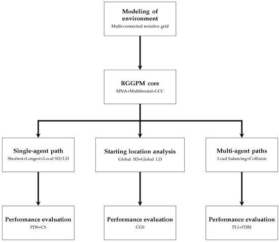
Figure 1.
Structural overview of the intelligent system framework.
Subsequently, several critical factors in logistics path optimization are addressed, including the shortest path, the longest path, the location of the starting point, and the coordination of the multi-agent system. Each of these items is examined by evaluating a logistics scenario for merchandise delivery. It is essential to note that determining the shortest path is crucial for minimizing delivery times and reducing energy consumption, while establishing the longest path is helpful for testing system capabilities and resource allocation strategies. Furthermore, the location of the starting point directly affects the efficiency of the entire delivery process, particularly in grids with multiple delivery points. Ultimately, the integration of multi-agent systems facilitates distributed problem-solving, allowing agents to communicate and collaborate to achieve optimal path planning, adapt to real-time changes, and circumvent obstacles.
During the exploration of these logistical factors, a set of KPIs is used to evaluate the effectiveness of path planning strategies. These KPIs offer valuable insights into operational efficiency, resource utilization, and delivery accuracy, making them essential for continuous improvement and data-driven decision-making in innovative logistics systems. Using the RGPPM approach, this research aims to establish a comprehensive and adaptable model for path planning in logistics environments.
It is important to mention that RGPPM has been positioned within the landscape of logistics optimization tools [18]. While classic graph-based algorithms and specialized vehicle routing problem (VRP) solvers excel at finding uniquely optimal routes under specific constraints, RGPPM offers a distinctive, physics-based paradigm for strategic logistics analysis. This methodology’s main strength is not based on replacing traditional methods, but rather on complementing them by providing a holistic view of the entire logistics network and exploring the possibility of finding indicators beyond the shortest route.
2.1. RGPPM as Intelligent Core Process
Since 2018, the Resistive Grid Path Planning Methodology (RGPPM) has emerged as a novel strategy offering reduced computational time for modeling and simulation in path planning. This deterministic methodology has successfully explored the sequence of movements from one point to another in robotic systems. However, for planning logistics trajectories in merchandise delivery, slight modifications are required.
Firstly, it is necessary to identify and geolocate the delivery points for merchandise to generate a multi-connected grid, as shown in Figure 2. In Figure 2a, ten delivery points have been georeferenced within the Veracruz–Boca del Río metropolitan area. Based on this set of locations, it is possible to generate a grid that connects each point with all other available positions, as illustrated in Figure 2b.
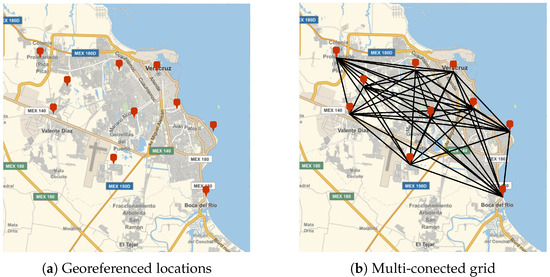
Figure 2.
Multi-connected grid using georeferenced locations.
After establishing the multi-connected grid using the georeferenced locations, it is necessary to convert it into a multi-connected resistive grid. To achieve this, each location is considered a node, and the straight-line connections between them are substituted with resistive elements, as shown in Figure 3.
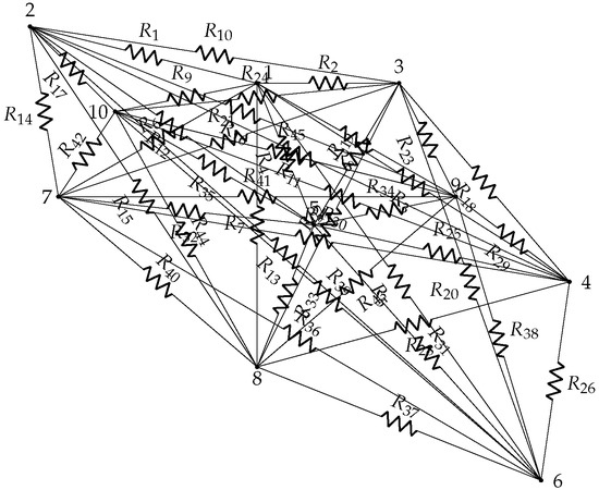
Figure 3.
Multi-connected resistive grid.
As shown in Figure 3, forty-five resistors have been incorporated into the grid. The resistance values of these elements are determined based on the distances between the merchandise delivery locations. For computing these distances, the Haversine formula is used, which estimates the distance between two points on the Earth’s surface. Table 1 shows the numerical values of the resistors (in ).

Table 1.
Resistor values for Figure 3.
Following the assignment of the resistive values to the elements of the grid, it is necessary to connect a set of power supplies to each of the nodes . All power supplies are set to 0 V, except for the one connected to the starting node for merchandise delivery. In the case shown in Figure 3, a 10 V power supply is connected to node 5.
From this configuration onward, the path planning methodology is capable of addressing three principal challenges: determining the shortest and longest paths, selecting the optimal starting point, and coordinating multiple agents.
2.2. Shortest and Longest Path
When the characterization stage of the resistive grid shown in Figure 3 has been reached, the formulation of the equilibrium equations is carried out using the procedure of Modified Nodal Analysis (MNA) [19], leading to the construction of a linear system of equations of the form that is solved using the Multifrontal method [20]. Once the nodal voltages of the resistive grid are obtained, the methodology is capable of estimating the local currents in the starting node with the following mathematical expression:
being the local current of the k-branch connected to the starting node, the resistance value of the k-branch, and the potential difference between the voltage of the starting node and that of the neighboring node connected by the k-branch.
Given that the starting node is connected to nine neighboring nodes through nine branches, nine local currents must be estimated using the expression in (1). Once these local currents are calculated, the branch with the highest current is identified through a numerical comparison.
After identifying the most conductive branch, the new location is updated to the corresponding neighboring node, and the power supply at this new node is set to 10V. From here, an iterative process begins: reformulating the equilibrium equations, estimating the local currents in the new node, and identifying the next branch with the most significant current. This iterative procedure continues until all locations in the resistive grid have been reached. It is essential to mention that the sequence of connections between nodes and their corresponding highest-current branches defines the shortest path for delivering merchandise.
Figure 4 shows the shortest path for delivering merchandise in a single path starting from a single location. According to the results, the starting node is number five, which generates a connection tree composed of the blue-highlighted resistors and a path sequence . The total length of this shortest path has been calculated around 45.22 km, as shown in Table 2.
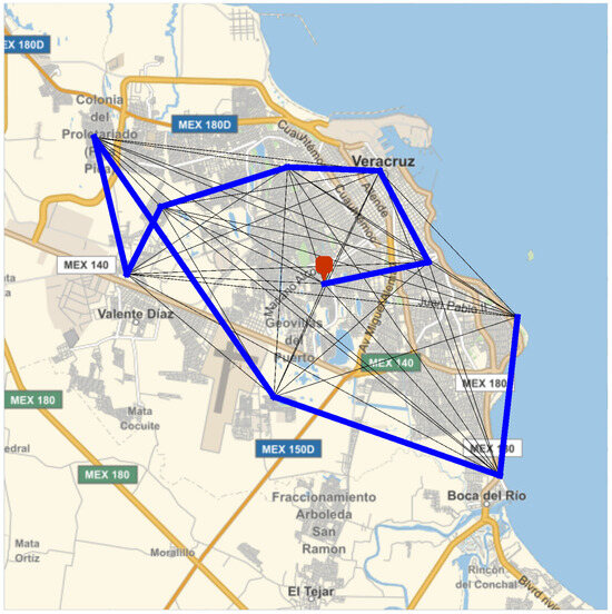
Figure 4.
Shortest path for delivering merchandise.
Table 2.
Shortest path metrics.
For the longest path case, the characterization stage of the resistive grid is carried out in the same way as in the shortest path, using Modified Nodal Analysis (MNA) and the Multifrontal method. However, the numerical comparison of all the local currents obtained from (1) must focus on identifying the smallest nonzero current, as opposed to the largest one used for the shortest path calculation.
Figure 5 shows the longest path for delivering merchandise in a single path and starting from a single location. According to the results, the starting node is node 5, which generates a connection tree formed by the resistors in red and a path sequence . The total length of the longest path has been estimated around 94.31 km, as shown in Table 3.
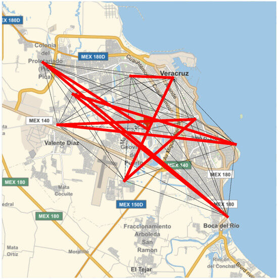
Figure 5.
Longest path for delivering merchandise.
Table 3.
Longest path metrics.
With the estimation of the shortest and longest paths for delivering merchandise using a simple path and a single starting location, the first key performance indicator for last-mile logistics with the RGPPM methodology has been defined as follows:
with PDS being the Percentage of Distance Savings, SD the shortest distance (in km), and LD the longest distance (in km).
According to the results shown in Figure 4 and Figure 5, PDS equals 52.05%. This indicates that the distance savings due to the use of RGPPM is approximately 52% compared to the worst-case scenario. PDS quantifies the efficiency of selecting the shortest possible path compared to the longest one. This is crucial for demonstrating tangible benefits in distance reduction, which are directly correlated with lower energy consumption, reduced emissions, and cost savings. This KPI provides a universal metric for comparing performance between different techniques.
Additionally, it is possible to establish a second key performance indicator related to the shortest path, the longest path, and the current path for last-mile logistics using the RGPPM methodology. This indicator calculates a performance coefficient that indicates how close the current path is to the optimal or worst-case scenario, using the following mathematical expression:
where CS is the Coefficient of Savings, and CD is the current distance (in km). Table 4 presents the classification categories for the numerical values of the CS KPI.
Table 4.
Classes for CS KPI.
CS quantifies the proximity of a path to the shortest and longest paths, thus offering insights into operational efficiency. This KPI is valuable for real-time decision-making, as it can inform path adjustments during active logistics operations. Moreover, its adaptive capability makes it relevant for various algorithms, ranging from heuristic methods to AI-driven optimizations, thereby enabling dynamic performance evaluation.
It is important to note that the classification ranges for the CS KPI are non-uniform to reflect a performance sensitivity scale. The intervals are narrower near the optimal (CS ≈ 0) and worst-case (CS ≈ 1) scenarios to provide high granularity for identifying near-optimal routes and critical inefficiencies, where small changes are most significant. The intervals are wider in the mid-range (CS ≈ 0.4–0.7), where the system is more tolerant to performance variations. This structure allows for more nuanced decision-making at the performance extremes.
2.3. Starting Location
Searching for strategic paths for delivering merchandise is strongly related to the starting location. RGPPM is capable of progressively changing the starting conditions to determine the shortest and longest paths across the entire resistive grid for merchandise delivery. Essentially, this challenge involves estimating the shortest and longest local paths from each potential starting location in the resistive grid, and subsequently selecting the overall shortest and longest global paths. Based on the characteristics of the resistive grid shown in Figure 2, it is possible to ensure that there are ten shortest local paths and ten longest local paths.
Figure 6 shows the evaluation of the lengths of the shortest and longest paths from different starting locations. As observed in Figure 6a, the shortest distance among the shortest local paths is obtained when starting at node 6, with a length of 35.39 km. Similarly, the longest distance among the longest local paths is reached when starting at node 9, with a length of 97.96 km, as shown in Figure 6b.
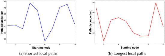
Figure 6.
Shortest and longest paths using different starting location.
Based on these global path length measurements, the KPI PDS can be recalculated, yielding a new value of 63.87%. This represents an additional savings of more than 10% compared to the previously calculated local PDS, highlighting the advantage of identifying optimal delivery paths by varying the starting location.
Finally, it is possible to define a third key performance indicator related to the shortest path, the longest path, and the different starting locations for last-mile logistics using the RGPPM methodology. This indicator measures a global performance coefficient that quantifies how closely the current path aligns with the global shortest and longest paths. The mathematical expression for this KPI is
where CGS is the Coefficient of Global Savings, GSD is the Global Shortest Distance, GLD is the Global Longest Distance, and CD is the Current Distance (in km). As with the CS KPI, different performance classes can be defined based on the numerical values of CGS. Table 4 can be adapted accordingly.
CGS extends the concept of the CS metric to a global level by incorporating variations in starting locations. This KPI is particularly valuable for assessing the strategic placement of distribution centers or warehouses. By optimizing starting points, companies can enhance overall grid efficiency, which has a significant impact on large-scale logistics operations.
2.4. Multi-Agents
Multi-agent trajectory planning is a field of artificial intelligence research that focuses on designing algorithms to plan and coordinate the actions of multiple agents in both simple and complex environments. It encompasses a wide variety of fields, from robotics and industrial automation to transportation systems and logistics.
Multi-agent path planning algorithms enable multiple agents to interact safely and efficiently in a shared environment, avoiding collisions and satisfying specific goals and constraints. These algorithms can also consider various factors, such as the size and shape of the agents, their maximum speed and acceleration, visibility, and communication limitations, among others. The pursuit of efficient decentralized coordination is a central challenge in them. RGPPM approach addresses this by using a physics-based model to implicitly coordinate agents via the circuit’s equilibrium state. This offers a distinct alternative to other decentralized strategies, such as the pivoting-based method for self-reconfigurable systems [21]. While methods like PO-SRPP often rely on local rules and geometric manipulations for modules in direct contact, RGPPM provides a global perspective derived from the electrical analogy, allowing for the simultaneous coordination of multiple independent agents in a connected grid and the inherent generation of system-wide performance metrics (KPIs).
Multi-agent systems [22] comprise multiple autonomous agents that make decisions while interacting within a shared environment to achieve common objectives. In this case, the use of multi-agents is applied to logistics for last-mile merchandise delivery. To implement this, RGPPM follows the steps described below:
First, it is necessary to determine the number of agents required to deliver the merchandise. Since all agents depart from a single location (the distribution center), the total number of delivery points is reduced by one to determine the number of possible divisions. Each division represents an alternative configuration for distributing routes in a balanced manner. In the case of the ten georeferenced locations from Figure 2a, this results in one valid division with three agents. Therefore, a balanced distribution of delivery locations is achieved, assigning an equal number of locations to each agent.
Once the starting point, the number of agents, and the number of delivery locations per agent have been defined, the process of transforming the georeferenced points into a multi-connected resistive grid is performed. Subsequently, the linear system is formulated using MNA, and the nodal voltages are computed, as previously described.
Finally, the logistics path search for the agents is conducted. To perform this, the local currents at the starting node are estimated using the expression in (1). Then, for the multi-agent case, the list of local currents is sorted from highest to lowest, and each agent selects the highest available current that does not lead to a node already assigned to another agent. This procedure continues until all agents have collectively covered all the delivery locations on the grid.
Figure 7 shows the logistical trajectories for the agents in the multi-connected grid from Figure 2. As previously mentioned, all agents begin their routes from a common starting point (in this case, node five), resulting in three connection trees formed by the resistor sets , , and . The corresponding path sequences and the local distances covered by each agent are shown in Table 5.
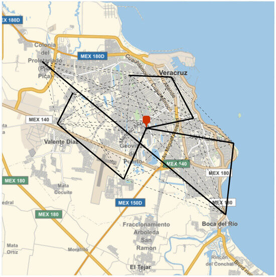
Figure 7.
Multi-agent paths for delivering merchandise.
Table 5.
Agent distances in multi-agent scenario.
And finally, the total length of the combined trajectories is 52.19 km.
Based on the estimation of the local path lengths for each agent, the fourth key performance indicator (KPI) for last-mile logistics using the RGPPM methodology can be defined as follows:
with PLI being the Percentage of Load Imbalance, LDA the Longest Distance for Agents (in km), SDA the Shortest Distance for Agents (in km), and ADA the Average Distance for Agents (in km).
According to the results shown in Figure 7 and the agents’ path lengths, the values of LDA, SDA, and ADA are calculated as 29.26, 10.01, and 17.39 km, respectively. Therefore, the PLI is 110.65%.
It is important to note that when PLI is close to 0%, the distances traveled by all agents are very similar, indicating an equal distribution of workload. Conversely, a high PLI value indicates a significant imbalance in distances traveled among agents, leading to unequal workload distribution.
High PLI values suggest that some agents are covering considerably longer distances than others, which increases energy consumption and accelerates wear on those agents.
PLI serves as a measure of workload distribution across multiple agents, helping ensure fair and efficient task allocation. This KPI is crucial in multi-agent systems, where imbalance can lead to inefficiencies, excessive energy consumption, and uneven resource allocation.
Additionally, a fifth key performance indicator can be defined, based on the total distance covered by all agents compared to the global shortest path, within the context of last-mile logistics using the RGPPM methodology. This indicator quantifies the percentage deviation between the multi-agent paths and the shortest possible global path from the exact starting location. The mathematical expression is as follows:
where PDM is the Percentage of Deviation with Multi-agent and MD is the Multi-agent Distance (in km).
In this case, MD = 52.19 km and GSD = 35.39 km; thus, PDM = 47.47%.
PDM quantifies the extent to which the total distance traveled by multiple agents deviates from the globally shortest possible path. This KPI is crucial for evaluating and refining the coordination of multi-agent systems, ensuring that overall performance remains closely aligned with optimal efficiency targets.
For ease of understanding, the key mathematical notations and KPIs introduced in this section are summarized in Table 6.
Table 6.
Summary of key mathematical notations.
3. Simulation Results
The National Commission for Free Textbooks (CONALITEG) is a non-centralized public body within the Federal Public Administration that produces and distributes free textbooks, established by the Secretary of Public Education (SEP), for students enrolled in the Mexican Educational System.
CONALITEG is responsible for delivering textbooks to the warehouses of state educational authorities, who then distribute them to individual schools.
Therefore, the governments of each Mexican state must design and implement logistics strategies for transporting textbooks from warehouses to public schools.
To address this task, the intelligent system proposed in this work was applied to a sample of 129 georeferenced locations corresponding to public elementary schools in the Veracruz–Boca del Río metropolitan area.
The aim was to develop energy-efficient paths and motion planning strategies for delivering textbooks in this urban region.
As shown in Figure 8, the georeferenced positions of elementary schools have been mapped in the Veracruz–Boca del Río metropolitan area. Additionally, a multi-connected grid was constructed based on these geospatial locations.
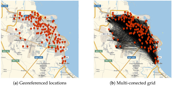
Figure 8.
Multi-connected grid using georeferenced locations from public elemental level schools.
This grid is then transformed into a multi-connected resistive network, where resistive values are assigned according to the distances between the nodes. Once the resistive grid has been characterized, it becomes necessary to identify the optimal starting position for textbook delivery.
To achieve this, the shortest and longest paths are estimated for each potential starting location, allowing for the selection of the most efficient delivery point.
Figure 9 displays the results for the shortest and longest delivery path distances (in kilometers) as the starting location varies. According to Figure 9a, the shortest local path is obtained when starting from node 119. Similarly, the longest local path originates from node 16, as illustrated in Figure 9b.
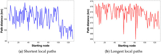
Figure 9.
Shortest and longest paths using different starting location in Figure 8.
Based on the identification of the starting nodes for the shortest and longest paths, the corresponding delivery sequences can be analyzed, as shown in Figure 10. According to the results, the shortest global route originates from node 119 and has an approximate length of 95.8 km. In contrast, the longest global path starts at node 16 and extends to about 977.5 km.
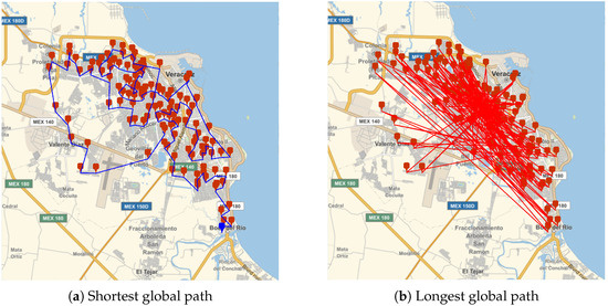
Figure 10.
Shortest and longest global paths for delivering textbooks.
Now, with the determination of the lengths for the shortest and longest paths, it is possible to estimate the value of PDS using (2). Given that SD = 95.8 km and LD = 977.5 km, as shown in Figure 9, the resulting PDS is 90.2%. This percentage indicates a substantial difference between the global shortest path and the worst-case scenario represented by the global longest path.
At this stage, it is also possible to estimate energy consumption and emissions during textbook delivery for both LD and SD values. To perform these estimations, the vehicle characteristics must first be defined, as presented in Table 7.
Table 7.
Vehicle characteristics.
According to Table 7, the vehicles considered are the 2022 Renault Traffic (diesel) and the Ruvian EDV 700 (electric). The energy consumption and emission characteristics of the Renault vehicle are based on manufacturer data. For the Ruvian vehicle, emissions were estimated using the emission factor from the Mexican National Electric System, published in 2021 by the Ministry of Environment and Natural Resources (SEMARNAT). This emission factor corresponds to 423 g of equivalent per kilowatt-hour. Additionally, the diesel price was set using the current average for the state of Veracruz, while the electricity price per kWh corresponds to the excess consumption tariff.
Table 8 shows the estimates of energy consumption, emissions (in kg), and economic cost in Mexican pesos for the global trajectories of the shortest (SD) and longest (LD) paths. It is essential to highlight the differences in performance between diesel and electric vehicles, both in terms of economic and environmental considerations. The Ruvian EDV demonstrates superior performance, emitting up to 30% less and significantly reducing operating costs in both scenarios.
Table 8.
Estimations for SD and LD paths.
Finally, the multi-agent strategy has been carried out for delivering textbooks in the Veracruz–Boca del Río area. To accomplish this, the agents’ starting location was set to node 119, as it corresponds to the shortest path in the global network. Additionally, the number of agents was configured into teams of 2, 4, 8, 16, 32, and 64. As shown in Figure 11, the logistical trajectories for the different groupings of agents have been generated. For each configuration, the total path length was calculated and is presented in Table 9.
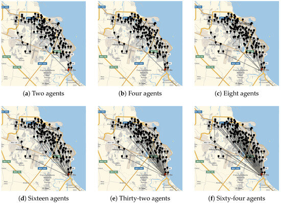
Figure 11.
Multi-agent paths for delivering textbooks.
Table 9.
Path length for agents.
Table 9 shows the path lengths for the different numbers of agents. It can be observed that the total distance traveled to deliver the textbooks increases as the number of agents increases.
Using this information and the value of GSD = 95.8 km, the Percentage of Deviation with Multi-agent (PDM) can be calculated for each configuration, as shown in Table 10.
Table 10.
PDM for agents.
In addition, based on the estimated local path lengths of the agents, the Percentage of Load Imbalance (PLI) KPI can be calculated, as shown in Table 11.
Table 11.
PLI for agents.
Eventually, Table 8 can be expanded by incorporating the vehicle characteristics presented in Table 7 and applying them to the multi-agent trajectories described in Table 9. Consequently, Table 12 shows the energy consumption, emissions, and associated costs for the multi-agent path lengths.
Table 12.
Estimations for multi-agent paths.
It is essential to note that the PLI KPI measures the gap in total travel distances (in kilometers) covered by individual agents, rather than an imbalance in the volume or weight of merchandise delivered. A high PLI indicates that some agents have been allocated longer routes than others, leading to unequal resource utilization and potential inefficiencies in energy consumption and time management.
Looking forward, to mitigate this load distance imbalance, a threshold-based dynamic reassignment mechanism should be explored. This strategy would operate in two phases: first, the standard multi-agent RGPPM would generate an initial solution. Second, if the resulting PLI exceeds a predefined tolerance threshold (e.g., 30–40%), an iterative balancing loop would be triggered. In this loop, the system would recalculate routes while dynamically incorporating the real-time accumulated distance of each agent. Agents with longer partial routes would be penalized during the path selection of subsequent iterations, promoting a more equitable distribution of travel distances and ensuring the final solution adheres to the desired balance criteria.
4. Discussion
Logistics has evolved from a straightforward supply process to a multifaceted system that reflects the growing demands and complexities of modern urban environments. Today, last-mile logistics faces unprecedented challenges due to increasing urbanization and environmental concerns over pollution levels. Traditional last-mile delivery methods, which often rely on gasoline-powered vehicles, exacerbate these challenges by contributing significantly to carbon emissions and air pollutants such as and , leading to negative impacts on both climate and public health. Although electric vehicles offer a promising alternative towards reducing direct emissions, their environmental benefits are limited by the dependence on fossil-fuel-based power grids and the ecological impact associated with lithium battery production. Therefore, it is essential for intelligent last-mile logistics systems to incorporate measurement strategies that assess the current performance of distribution grids, intending to reduce emissions and improve energy efficiency.
A critical feature of deploying path planning methodologies in large-scale logistics is its computational scalability. Traditional methods for solving the systems of equilibrium equations derived from MNA, such as those used in standard circuit simulators (e.g., SPICE), typically exhibit a computational complexity of for the matrix factorization step, where N is the number of nodes in the grid. This cubic complexity poses a significant bottleneck, making these methods impractical for large networks as the computation time becomes exceedingly long. In contrast, the RGPPM methodology strategically employs the Multifrontal method (via UMFPACK) [23] to solve the sparse linear system . This method is a highly efficient sparse direct solver that exploits the inherent sparsity and the planar structure of the grid-based MNA matrix. As it has been established in [20,24], the computational complexity of the multifrontal method for solving systems arising from two-dimensional planar graphs is approximately . This represents a substantial reduction from the complexity of dense solvers and it is the foundational reason for the scalability of the RGPPM, as confirmed by the prior empirical results in [25].
RGPPM’s strength lies in its ability to identify optimal and suboptimal delivery paths, determine strategic starting points, and support the coordination of multi-agent systems. Knowing the shortest path for deliveries optimizes route efficiency, resulting in lower fuel consumption and reduced delivery times—key factors for minimizing operational costs and environmental impacts. Furthermore, the methodology’s capacity to evaluate the longest possible paths acts as a stress test for system resilience, ensuring robust logistics performance even under adverse conditions. Its multi-agent features enable decentralized decision-making, allowing agents to adapt in real-time and avoid congestion, thereby enhancing overall system flexibility.
The five KPIs—Percentage of Distance Savings (PDS), Coefficient of Savings (CS), Coefficient of Global Savings (CGS), Percentage of Load Imbalance (PLI), and Percentage of Deviation with Multi-agent (PDM)—introduced in this research provide a robust framework for evaluating the efficiency and effectiveness of last-mile logistics operations. These indicators extend beyond the scope of RGPPM and offer value to a wide range of path planning and logistics optimization techniques. By providing standardized metrics for benchmarking, they foster methodological comparison and support the development of more efficient algorithms. Furthermore, these KPIs can be integrated into real-time monitoring systems to generate actionable insights that promote ongoing improvement and adaptability across diverse logistical contexts, including urban, suburban, and rural environments. Despite their advantages, effective implementation of these KPIs poses the following challenges:
- ▪
- Data: KPIs require access to accurate, high-quality, and real-time data on distances, energy consumption, and agent performance to ensure their reliability, especially in dynamic and unpredictable urban environments [26].
- ▪
- Scalability: Scaling the use of KPIs to large and complex logistics grids involving numerous agents may introduce significant computational and coordination challenges [27].
- ▪
- Integration with existing systems: Integrating these KPIs into conventional logistics frameworks may require substantial adaptations in infrastructure, data acquisition methods, and algorithmic compatibility [28].
Therefore, it is possible to state that the application of these KPIs transcends the RGPPM methodology and offers potential benefits for a wide range of techniques in the logistics literature.
As part of this research, a formal request for access to public information was submitted to the Secretary of Education of the State of Veracruz, seeking data on the logistical procedures for the delivery of free textbooks at the elementary level during the 2019–2020, 2020–2021, 2021–2022, and 2022–2023 academic periods. Additionally, information regarding fuel consumption associated with the distribution process was requested.
In response, the Undersecretary of Educational Development of the State of Veracruz, through the State Coordination of Support for Educational Improvement, reported that textbook distribution is carried out by official educational personnel, including sector chiefs, school supervisors, and principals. These personnel must travel from their schools to one of nineteen regional warehouses to collect the textbooks and then return to their respective institutions to complete the distribution.
However, the request for fuel consumption data was left unanswered, with the state authority indicating that such information is the responsibility of the Federal Government. Conversely, the Federal Government, through the General Directorate of Educational Materials, asserted that this information falls under the jurisdiction of the State of Veracruz. This bureaucratic impasse suggests that fuel consumption and pollutant emissions related to textbook distribution are not considered priorities in current Mexican public policy.
Based on the official logistics process described and the specific case of the 129 georeferenced locations of public elementary schools in the Veracruz–Boca del Rio area, it is possible to reconstruct the trajectory grid used for textbook collection, as shown in Figure 12.
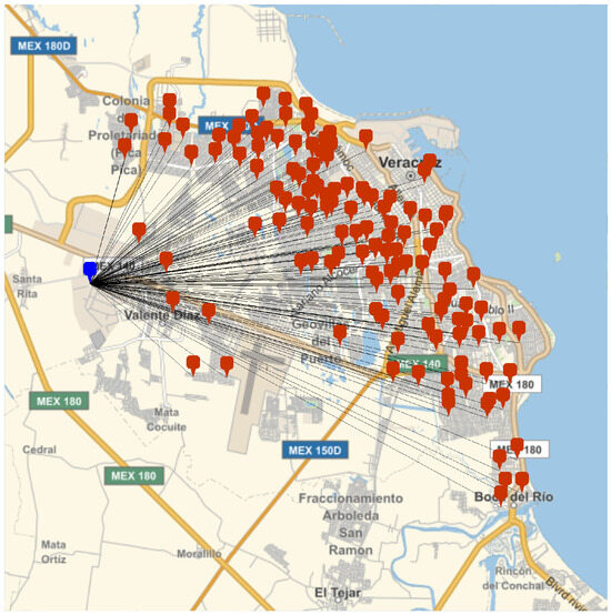
Figure 12.
Federal government’s logistics strategy for delivering textbooks.
It is essential to note that the Federal Government’s logistics strategy for delivering free textbooks in the Veracruz–Boca del Río area requires vehicles to cover a total distance of 2437 km. This distance is nearly three times greater than the longest global path estimated using the RGPPM methodology, as shown in Figure 10b. In contrast, the energy-efficient last-mile logistics strategy based on RGPPM demonstrates a significant reduction in distance, with up to 96% using a single agent and 93% with eight agents, as illustrated in Figure 10a and Figure 11c, respectively.
Moreover, it is possible to estimate the energy consumption, emissions, and associated costs of the Federal Government’s current delivery strategy. Using the vehicle characteristics established in Table 7, the corresponding estimates are presented in Table 13.
Table 13.
Estimations for the federal government’s strategy.
It is essential to mention that the emission of 448.40 kg of is approximately equivalent to the amount of carbon dioxide that twenty-one adult trees can absorb in one year.
Finally, the significant reductions in energy consumption and emissions demonstrated in this case study position the RGPPM as a concrete technological pathway for decarbonizing last-mile logistics. This aligns directly with broader carbon neutrality frameworks for industrial economies [7,29], which identify transportation and logistics as key leverage points for emission reductions. The methodology provides a quantifiable and scalable strategy for companies and policymakers to transition towards net-zero supply chains, moving beyond theoretical commitments to implementable, data-driven solutions that directly contribute to nationally determined contributions and corporate carbon neutrality targets.
5. Conclusions
This work has presented an intelligent path planning methodology for last-mile logistics based on the Resistive Grid Path Planning Methodology (RGPPM). Using a multi-connected model of georeferenced nodes and distance-proportional resistances, the methodology established optimized logistical routes for both diesel and electric vehicles, demonstrating significant improvements in energy efficiency, emissions reduction, and operating costs. Additionally, the system introduced five key performance indicators (KPIs) that enabled the quantitative assessment of the generated paths under various distribution scenarios.
Simulation results from the case study—textbook distribution in 129 public schools in Veracruz–Boca del Río—demonstrated that RGPPM-based planning reduced the total travel distance by up to 96% compared to the traditional government strategy, representing a substantial improvement in sustainability and operational performance. Moreover, electric vehicles outperformed diesel vehicles, achieving reductions of up to 70% in carbon emissions and over 70% in energy-related costs. Furthermore, the PLI and PDM indicators helped identify load imbalances and route deviations in multi-agent scenarios, opening up the possibility of further optimizing agent-based route allocation.
Despite the robustness of the proposed approach, certain limitations remain that offer guidance for future research. Due to the fact that the current intelligent system operates under static conditions and does not incorporate critical real-world dynamic constraints, it is necessary to establish a research path for the transition of RGPPM from a strategic planning tool to a dynamic logistics optimization framework. In order to do this, future work should focus on the following challenges:
- ▪
- Dynamic constraints on vehicle capacity and load [30]: A fixed resistive network can be extended to a dynamic network model where resistance values modulate based on an agent’s current load. As a vehicle delivers its payload, the local resistances connected to its node decrease, making it a more attractive path for other agents and therefore imposing capacity limits while promoting load balancing in the multi-agent system.
- ▪
- Integration of time windows and traffic conditions [30]: In order to model time-dependent routing, the framework can incorporate time-varying resistance values. This opens the possibility of simulating traffic congestion (e.g., increased resistance during peak hours) and the application of handover windows. The resistances associated with a node could become highly resistive outside of their allowed time window, thus blocking late access. Integration with real-time traffic data APIs is a straightforward way to introduce these dynamic resistance values.
In accordance with the above challenges, the idea of a dynamic resistive grid, where the resistance value along a path increases or decreases according to the constraints of a real-world environment, should be considered as a natural extension of the physical model. Unlike other methods that require complex additional layers of constraint programming, RGPPM can integrate the capability directly into the physics of the model, while maintaining its computational efficiency. In order to achieve the incorporation of dynamic constraints, RGPPM must strategically explore the use of memristors [31,32] in the resistive grid because they are elements that dynamically change the resistive value based on the history of current that has flowed through it [33].
Author Contributions
Conceptualization, C.H.-M.; data curation, E.E.G.-G.; formal analysis, D.T.-M.; funding acquisition, E.I.-G.; investigation, C.S.-L.; methodology, C.H.-M. and S.H.-M.; project administration, E.I.-G.; resources, E.E.G.-G.; software, D.T.-M. and C.M.-M.; supervision, E.E.G.-G. and E.I.-G.; validation, S.H.-M. and C.S.-L.; visualization, E.I.-G. and E.E.G.-G.; writing—original draft, C.H.-M.; writing—review and editing, E.I.-G. and E.E.G.-G. All authors have read and agreed to the published version of the manuscript.
Funding
This research was funded by the Universidad Autónoma de Baja California (UABC) through the 25th internal call for research projects with grant number 402/6/C/53/25.
Data Availability Statement
The original contributions presented in the study are included in the article, further inquiries can be directed to the corresponding author.
Acknowledgments
The authors thank the editors and reviewers of this manuscript.
Conflicts of Interest
The authors declare no conflicts of interest. The founding sponsors had no role 571 in the design of the study, in the collection, analysis, or interpretation of data, in the writing of the 572 manuscript, or in the decision to publish the results.
References
- Zijm, H.; Klumpp, M.; Regattieri, A.; Heragu, S.; Regattieri, A. Operations, Logistics and Supply Chain Management; Springer: Berlin/Heidelberg, Germany, 2019. [Google Scholar] [CrossRef]
- Gleissner, H.; Femerling, J. Logistics: Basics Exercises Case Studies; Springer: Berlin/Heidelberg, Germany, 2014. [Google Scholar] [CrossRef]
- Rushton, A.; Croucher, P.; Baker, P. The Handbook of Logistics and Distribution Management: Understanding the Supply Chain, 7th ed.; Kogan Page: London, UK, 2022. [Google Scholar]
- Fahimnia, B.; Bell, M.; Hensher, D.; Sarkis, J. Green Logistics and Transportation: A Sustainable Supply Chain Perspective; Springer: Berlin/Heidelberg, Germany, 2015. [Google Scholar] [CrossRef]
- Psaraftis, H. Green Transportation Logistics: The Quest for Win-Win Solutions; Springer: Berlin/Heidelberg, Germany, 2016. [Google Scholar] [CrossRef]
- Festini, A.; Roth, D. The Last Mile Problem and Its Innovative Challengers. In Disrupting Logistics: Startups, Technologies, and Investors Building Future Supply Chains; Wurst, C., Graf, L., Eds.; Springer: Berlin/Heidelberg, Germany, 2021; pp. 79–91. [Google Scholar] [CrossRef]
- World Economic Forum. Net-Zero Challenge: The Supply Chain Opportunity; In collaboration with Boston Consulting Group; World Economic Forum: Geneva, Switzerland, 2021. [Google Scholar]
- Tran, T.; Dinh Thi, T.B. Impacts of Last Mile Delivery on Environment in Urban Areas: Hanoi Case Study. In CIGOS 2021, Emerging Technologies and Applications for Green Infrastructure; Ha-Minh, C., Tang, A.M., Bui, T.Q., Vu, X.H., Huynh, D.V.K., Eds.; Springer: Singapore, 2021; pp. 1653–1661. [Google Scholar]
- Xiaohong, J.; Ma, J.; Zhu, H.; Guo, X.; Huang, Z. Evaluating the Carbon Emissions Efficiency of the Logistics Industry Based on a Super-SBM Model and the Malmquist Index from a Strong Transportation Strategy Perspective in China. Int. J. Environ. Res. Public Health 2020, 17, 8459. [Google Scholar] [CrossRef]
- Grondys, K. The impact of freight transport operations on the level of pollution in cities. Transp. Res. Procedia 2019, 39, 84–91. [Google Scholar] [CrossRef]
- Manojlovic, A.; Medar, O.; Andelkovic, A.; Tomic, M. Environmental impact assessment of the electric vehicles: A case study. Energy Sources Part A Recover. Util. Environ. Eff. 2023, 45, 1007–1016. [Google Scholar] [CrossRef]
- Albrechtowicz, P. Electric vehicle impact on the environment in terms of the electric energy source Case study. Energy Rep. 2023, 9, 3813–3821. [Google Scholar] [CrossRef]
- Glitman, K.; Farnsworth, D.; Hildermeier, J. The role of electric vehicles in a decarbonized economy: Supporting a reliable, affordable and efficient electric system. Electr. J. 2019, 32, 106623. [Google Scholar] [CrossRef]
- Raza, H.; Bai, S.; Cheng, J.; Majumder, S.; Zhu, H.; Liu, Q.; Zheng, G.; Li, X.; Chen, G. Li-S Batteries: Challenges, Achievements and Opportunities. Electrochem. Energy Rev. 2023, 6, 29. [Google Scholar] [CrossRef]
- Li, B.; Wang, X.; Khurshid, A.; Saleem, S. Environmental governance, green finance, and mitigation technologies: Pathways to carbon neutrality in European industrial economies. Int. J. Environ. Sci. Technol. 2025, 22, 14899–14912. [Google Scholar] [CrossRef]
- Ben Jmaa, Y.; Duvivier, D. A Review of Path Planning Algorithms. In Proceedings of the 23rd International Conference on Intelligent Systems Design and Applications ISDA 2023, Online, 11–13 December 2023; Abraham, A., Bajaj, A., Hanne, T., Siarry, P., Ma, K., Eds.; Springer: Berlin/Heidelberg, Germany, 2024; pp. 119–130. [Google Scholar] [CrossRef]
- Fang, Q.; Sun, Q.; Ge, J.; Wang, H.; Qi, J. Multidimensional Engineering of Nanoconfined Catalysis: Frontiers in Carbon-Based Energy Conversion and Utilization. Catalysts 2025, 15, 477. [Google Scholar] [CrossRef]
- Hernández-Mejía, C.; Torres-Muñoz, D.; Inzunza-González, E.; Sánchez-López, C.; García-Guerrero, E.E. A Novel Green Logistics Technique for Planning Merchandise Deliveries: A Case Study. Logistics 2022, 6, 59. [Google Scholar] [CrossRef]
- Ho, C.W.; Ruehli, A.; Brennan, P. The modified nodal approach to network analysis. IEEE Trans. Circuits Syst. 1975, 22, 504–509. [Google Scholar] [CrossRef]
- Davis, T.A. Direct Methods for Sparse Linear Systems; SIAM: Philadelphia, PA, USA, 2006. [Google Scholar] [CrossRef]
- Ye, D.; Wang, B.; Wu, L.; Del Rio-Chanona, E.A.; Sun, Z. PO-SRPP: A Decentralized Pivoting Path Planning Method for Self-Reconfigurable Satellites. IEEE Trans. Ind. Electron. 2024, 71, 14318–14327. [Google Scholar] [CrossRef]
- Dorri, A.; Kanhere, S.S.; Jurdak, R. Multi-Agent Systems: A Survey. IEEE Access 2018, 6, 28573–28593. [Google Scholar] [CrossRef]
- Davis, T.A. Algorithm 832: UMFPACK V4.3-an unsymmetric-pattern multifrontal method. ACM Trans. Math. Softw. 2004, 30, 196–199. [Google Scholar] [CrossRef]
- Davis, T.A.; Rajamanickam, S.; Sid-Lakhdar, W.M. A survey of direct methods for sparse linear systems. Acta Numer. 2016, 25, 383–566. [Google Scholar] [CrossRef]
- Hernández-Mejía, C.; Vázquez-Leal, H.; Sánchez-González, A.; Corona-Avelizapa, Á. A Novel and Reduced CPU Time Modeling and Simulation Methodology for Path Planning Based on Resistive Grids. Arab. J. Sci. Eng. 2019, 44, 2321–2333. [Google Scholar] [CrossRef]
- Mourtzis, D.; Angelopoulos, J.; Panopoulos, N. A Literature Review of the Challenges and Opportunities of the Transition from Industry 4.0 to Society 5.0. Energies 2022, 15, 6276. [Google Scholar] [CrossRef]
- Koç, Ç.; Laporte, G.; Tükenmez, İ. A review of vehicle routing with simultaneous pickup and delivery. Comput. Oper. Res. 2020, 122, 104987. [Google Scholar] [CrossRef]
- Ivanov, D.; Dolgui, A.; Das, A.; Sokolov, B. Digital Supply Chain Twins: Managing the Ripple Effect, Resilience, and Disruption Risks by Data-Driven Optimization, Simulation, and Visibility. In Handbook of Ripple Effects in the Supply Chain; Springer: Berlin/Heidelberg, Germany, 2019. [Google Scholar] [CrossRef]
- IPCC. Climate Change 2022—Mitigation of Climate Change: Working Group III Contribution to the Sixth Assessment Report of the Intergovernmental Panel on Climate Change; Cambridge University Press: Cambridge, UK, 2023. [Google Scholar] [CrossRef]
- Merchán, D.; Arora, J.; Pachon, J.; Konduri, K.; Winkenbach, M.; Parks, S.; Noszek, J. 2021 Amazon Last Mile Routing Research Challenge: Data Set. Transp. Sci. 2024, 58, 8–11. [Google Scholar] [CrossRef]
- Chua, L. Memristor-The missing circuit element. IEEE Trans. Circuit Theory 1971, 18, 507–519. [Google Scholar] [CrossRef]
- Chua, L.; Kang, S.M. Memristive devices and systems. Proc. IEEE 1976, 64, 209–223. [Google Scholar] [CrossRef]
- Hernández-Mejía, C.; Sarmiento-Reyes, A.; Vázquez-Leal, H. A Novel Modeling Methodology for Memristive Systems Using Homotopy Perturbation Methods. Circuits Syst. Signal Process. 2017, 36, 947–968. [Google Scholar] [CrossRef]


Disclaimer/Publisher’s Note: The statements, opinions and data contained in all publications are solely those of the individual author(s) and contributor(s) and not of MDPI and/or the editor(s). MDPI and/or the editor(s) disclaim responsibility for any injury to people or property resulting from any ideas, methods, instructions or products referred to in the content. |
© 2025 by the authors. Licensee MDPI, Basel, Switzerland. This article is an open access article distributed under the terms and conditions of the Creative Commons Attribution (CC BY) license (https://creativecommons.org/licenses/by/4.0/).