Abstract
This study addresses the limitations of traditional coal calorific value prediction models, which primarily rely on linear regression and single-source proximate analysis data. Based on 465 Chinese coal samples and integrating proximate analysis, ultimate analysis, and constructed derived indicators (combustible content—CC, carbon–hydrogen index—CHI, carbon in combustibles—CIC), a nonlinear modeling method combining mean impact value (MIV) feature selection and support vector regression (SVR) is proposed. The results show that the Pearson correlation coefficients between the derived indicators and net calorific value (NCV) all exceed 0.93, outperforming the original items. Using CC–CHI–CIC–FCad as characteristic variables, the established SVR model achieved a mean absolute percentage error (MAPE), root mean square error (RMSE), and coefficient of determination (R2) of 1.838%, 0.544 MJ/kg, and 0.962, respectively, with exceptionally high statistical significance (F = 1485.96, p < 0.001). The predictive accuracy of this model is significantly superior to traditional linear models, while the proposed linear model based on the derived indicators (R2 > 0.900) can serve as an alternative for rapid estimation. This method effectively enhances the accuracy and robustness of coal calorific value prediction.
1. Introduction
The calorific value of coal refers to the amount of heat released when a unit mass of coal is completely burned. The calorific value is often reported as either the higher heating value, which includes the latent heat of vaporization of water in the combustion products, or the lower heating value (also known as net calorific value), which excludes it [1]. In the process of coal production and trade settlement, net calorific value is increasingly used for evaluating coal quality. As one of the most important indicators of coal quality, the calorific value not only determines the value of coal products but also significantly influences coal deep-processing and utilization processes [2,3]. Currently, the determination of coal’s calorific value primarily relies on analytical testing methods such as the oxygen bomb method, which has limitations in industrial applications such as coal blending or online calorific value prediction [4]. These methods are time-consuming, costly, and difficult to adapt for real-time monitoring, making them unable to meet the demands of coal blending optimization or real-time combustion process control. To address these shortcomings, researchers have conducted extensive “soft measurement” studies on the prediction and modeling of coal’s calorific value. This “soft measurement” approach not only significantly reduces testing time and lowers costs, but can also be integrated into production line systems to achieve online estimation and prediction of calorific value, thereby providing critical parameter support for the optimized control of coal utilization processes.
Following a long line of research on coal calorific value prediction, Mason and Given et al. [5,6] in the 1980s established a multivariate linear regression model based on proximate and ultimate analysis results. Kucukbayrak et al. [7] utilized proximate analysis data from 24 sets of Turkish brown coal, and employed the least squares regression method to construct a regionalized calorific value prediction model. The average relative error between the calculated value and the measured value is 3.78% to 7.56%. Majumder et al. [8] established a calorific value prediction model using multiple linear regression based on 250 sets of Indian coal proximate analysis data, with an average relative error of 1.49%. Chelgani et al. [9] established a multiple linear prediction model for calorific value based on proximate analysis and ultimate analysis using linear regression based on 83 sets of Afghan coal quality data. Akhtar [10] established a multiple linear regression model to predict the calorific value of high-ash brown coal in Pakistan based on data from four regions, including Khushab. The model was validated through variance analysis and error testing, which indicated that the three-variable model (volatile matter, ash content, and fixed carbon) and the two-variable model (ash content/fixed carbon) yielded the lowest error. Mesroghli et al. [11] used data from 4540 coal samples from the United States to regression and artificial neural networks (ANN) to predict calorific value. The regression results showed the best prediction, with minimum and maximum errors of −23.6% and +11.9%, respectively. Although the above linear modeling methods achieved satisfactory prediction results, they are mostly limited to a single coal type in a specific mining area or region, with restricted application scope. Particularly, when faced with special situations such as the calorific value calibration of port coal from complex sources, the limitations of such prediction methods become even more pronounced.
Studies by Patel and Mesroghli et al. [11,12] have shown that the calorific value of coal from different origins is not completely linearly correlated with proximate analysis and ultimate analysis items. In particular, the moisture content, volatile matter, nitrogen and hydrogen in coal have a nonlinear discrete relationship with calorific value. Khandelwal et al. [13] employed ANN combined with proximate and ultimate analysis of coal to efficiently predict the concentration of microscopic components in Indian coal. Compared with traditional multiple regression analysis (MVRA), ANN demonstrated higher prediction accuracy (the R2 values for vitrinite, liptinite, and inertinite were 0.9684, 0.9500, and 0.9602, respectively) and lower error rates. Mondal et al. [14] utilized machine learning models such as XGBoost to predict calorific value using coal proximate analysis parameters (moisture content, volatile matter, etc.) The results indicated that the XGBoost model performed optimally (R2 = 99.87%). Akkaya et al. [15] proposed a combined equation for coal calorific value prediction through a two-stage modeling approach (GMDH neural network). In the first stage, a high-precision single equation was developed based on near-quality analysis. In the second stage, the top three optimal models were integrated to construct a combined equation, which was validated using 8501 coal sample data, significantly improving the prediction performance. Kavsek et al. [16] used multiple linear regression and ANN methods based on proximate analysis items to model and predict the calorific value of Slovenian coal, with a relative average deviation of less than 2%. Tan Peng et al. [17] based their study on proximate analysis data from 167 samples of Chinese coal and 4540 samples of American coal. They then utilized the support vector regression (SVR) method to predict and model coal calorific values, finding that the SVR calorific value prediction model was more accurate than conventional linear regression methods.
Akkaya [18] employed Gaussian process regression (GPR) to construct a global prediction model for the high heating value (HHV) of coal. The results demonstrate that the GPR model (test set R2 = 0.9833, error 2.5%) significantly outperforms traditional multiple linear regression (MLR), validating its effectiveness as a high-precision HHV prediction tool. Li et al. [19] proposed a sparse online multi-output LS-SVR algorithm for modeling multi-input multi-output systems. Experiments show that compared to traditional methods, this algorithm reduces the number of support vectors by about 50%. while maintaining a similar root mean square error (RMSE).
It is evident that calorific value prediction methods based on nonlinear modeling concepts such as SVR and ANN are gradually replacing traditional linear modeling methods, and their prediction results are more accurate and applicable to a wider range of cases [20]. Although the aforementioned studies primarily rely on proximate analysis or regional data for modeling, it is a well-established consensus in academia that the calorific value of coal is essentially determined by its elemental composition and the thermodynamic characteristics of the combustion process [21]. To accurately predict the calorific value of solid fuels, numerous studies have been dedicated to developing correlation models based on ultimate analysis. The review by Channiwala and Parikh [22] systematically organizes classical equations in this field and proposes a unified correlation for predicting the higher heating value based on the elemental composition of fuels.
Among the many classical equations, the most representative is the Dulong formula [23]. Derived from coal characteristics, it is based on relevant combustion reactions and the concept of effective hydrogen. Its prediction accuracy for low-oxygen coals is approximately ±1.5%, while the prediction deviation for high-oxygen coals can be as high as 5–7%. Subsequent research has conducted in-depth expansions on this basis. The improved models developed by Strache and Lant [24], based on the Dulong formula, achieved prediction errors for the higher heating value of less than 2% across the entire range of coal types. Meanwhile, Wilson [25] proposed a correlation for municipal solid waste based on thermochemical principles, the calorific values of carbon and sulfur, the types of carbon present, and the formation process.
It is important to note that most of these traditional correlations were established for the organic matter of coal on a dry, ash-free basis. When applied to fuels with special compositions (such as high-carbon coke, graphite, etc.), their predictive performance can show significant deviations [21,22]. This reveals the inherent limitations of traditional methods in covering all types of solid fuels and highlights the urgent need to develop more universal prediction models.
Mesroghli et al. [11] clearly demonstrated that incorporating ultimate items such as carbon (C), hydrogen (H), and oxygen (O) into an artificial neural network model significantly surpassed the predictive accuracy for calorific value compared to models relying solely on proximate analysis data. This is primarily because oxygen (O) content exhibits a strong negative correlation with calorific value [26], while hydrogen (H) content contributes importantly to it due to its high combustion energy. Parikh et al. [27] also indicated that although formulas based on proximate analysis are more convenient, their predictive accuracy ceiling is generally lower than that of models based on ultimate analysis. Chelgani et al. [28] found that the content of ultimate such as carbon, hydrogen, and oxygen significantly affects the calorific value of coal, with carbon content playing a decisive role. Therefore, omitting ultimate analysis data equates to losing these critical chemical structural insights, potentially preventing the model from accurately capturing the intrinsic chemical essence influencing calorific value. Additionally, during the construction of calorific value prediction models, most researchers failed to screen and select the validity of model input features, instead relying on subjective experience to arbitrarily choose or exclude independent variables, leading to redundancy or omission of certain model features.
As discussed earlier, researchers both domestically and internationally have constructed various forms of linear regression models for calorific value prediction under different conditions. These models can be categorized into three types: calorific value prediction models based on proximate analysis, calorific value prediction models based on ultimate analysis, and hybrid prediction models combining proximate analysis and ultimate analysis items. Typical linear regression models are shown in Table 1.

Table 1.
Typical linear regression model of coal calorific value prediction.
In summary, although nonlinear machine learning methods have demonstrated significant potential in calorific value prediction, existing studies still exhibit two notable shortcomings. First, model inputs predominantly rely on proximate analysis items, while neglecting ultimate analysis data equates to losing critical chemical structural information, which may prevent the models from accurately capturing the intrinsic chemical essence that influences calorific value. Second, during the construction of calorific value prediction models, most researchers fail to screen the validity of input features, instead relying on subjective experience to arbitrarily select or exclude independent variables, leading to redundancy or omission of certain model features. To address these issues, this study, based on 465 coal quality analysis samples collected from different regions in China, innovatively introduces three derived indicators: Combustible Content (CC), Carbon-Hydrogen Index (CHI), and Carbon in Combustibles (CIC). It simultaneously considers the influence of proximate analysis items, ultimate analysis items, and these three derived indicators on calorific value. A method combining characteristic variable selection with Support Vector Regression (SVR) is employed to model and predict coal calorific value.
2. Materials and Methods
2.1. Nonlinear Relationship Between Proximate Analysis, Ultimate Analysis Items, and Calorific Value
The coal quality index data used in this calorific value prediction were collected from the Inner Mongolia, Shanxi, Shaanxi, and Xinjiang Uygur Autonomous Regions in China. The coal samples are predominantly low-rank coal, including lignite, long-flame coal, non-caking coal, and so on. The sample collection locations are shown in Figure 1. In Figure 1, 252 datapoints of coal quality sample data were collected from Inner Mongolia, 77 datapoints from Shanxi, 95 datapoints from Shaanxi, and 41 datapoints from Xinjiang, for a total of 465 datapoints.
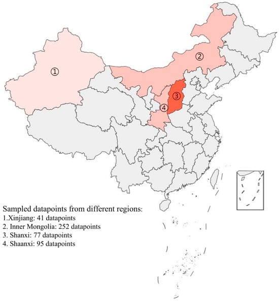
Figure 1.
Distribution of coal sample collection sites.
The sample data include proximate analysis items, ultimate analysis items, and net calorific value, as shown in Table 2. Table 2 uses Mad, Aad, VMad, and FCad to represent moisture, ash, volatile matter, and fixed carbon in proximate analysis, respectively, while Cad, Had, Nad, Sad, and Oad represent the contents of the five elements—carbon, hydrogen, nitrogen, sulfur, and oxygen—in ultimate analysis. The calibration standard for calorific value is net calorific value (NCV) [29]. Unless otherwise specified, NCV represents the net calorific value on the air-dried basis in the construction of the calorific value prediction model.
Table 2.
Samples used for calorific value prediction.
During sample collection, there were some differences in the reference standards used for coal quality indexes across different regions. Some of the data use proximate analysis and ultimate analysis items based on the air-dried basis (ad) [30]; others use the as-received basis (ar) [31]; and a portion use the dry-ash-free basis (daf) [32]. To ensure the accuracy of modeling and prediction results, some coal quality indexes need to be uniformly converted to air-dried basis indicators.
Based on Table 2, scatter plots of Mad, Aad, VMad, FCad, Cad, Had, Nad, Sad, Oad, and NCV were generated to examine the linear correlation between each coal quality index and calorific value, as shown in Figure 2.
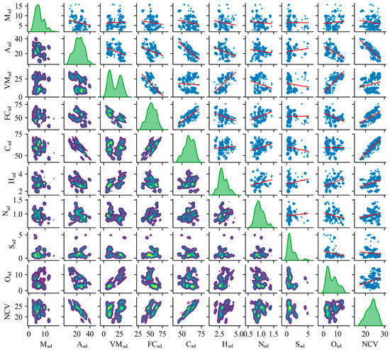
Figure 2.
Linear correlation between various coal quality indexes and NCV.
As shown in Figure 2, the off-diagonal subplots display the bivariate relationships between different coal quality parameters, where the red line represents the linear regression fit. The diagonal subplots show the univariate kernel density estimation for each variable, illustrating its distribution profile (e.g., skewness, modality) instead of a trivial perfect linear relationship with itself. The analysis of this figure reveals that only Aad and Cad exhibit moderate linear correlation with NCV, while the remaining indicators show poor linear correlation with NCV. Additionally, the linear correlation among the nine items of coal-Mad, Aad, VMad, FCad, Cad, Had, Nad, Sad, and Oad is also relatively low.
To further investigate the linear correlation between various coal quality indexes and calorific value, Pearson correlation analysis was employed to quantitatively describe the linear correlation between the parameters [33]. The Pearson correlation matrix was calculated based on the coal quality data in Table 2, as shown in Figure 3.
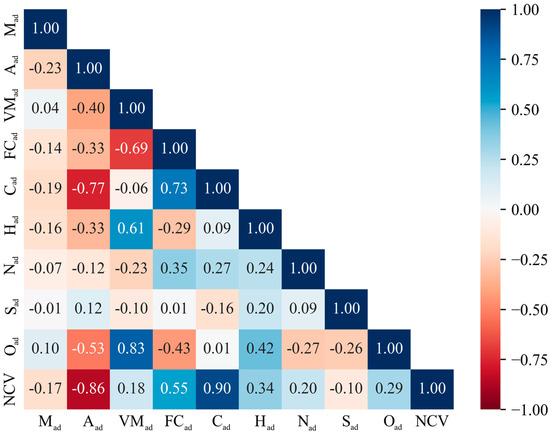
Figure 3.
Pearson correlation analysis between various items.
In Figure 3, the closer the Pearson correlation coefficient is to 1, the stronger the linear correlation between the two items. When the correlation coefficient is positive, the two are positively correlated; when the correlation coefficient is negative, the two are negatively correlated [34]. Based on this, it can be observed that among the items of coal’s proximate analysis and ultimate analysis, only the correlation coefficients between Aad and NCV and between Cad and NCV are greater than 0.85, indicating a certain degree of linear correlation, while the correlation coefficients between the remaining items and NCV are all below 0.60, indicating weak linear correlation. Therefore, when predicting calorific value based on proximate analysis and ultimate analysis, nonlinear modeling methods should be prioritized.
2.2. Derived Indicators Based on Proximate Analysis and Ultimate Analysis Items
Although the linear correlation between the original coal quality indexes (Mad, Aad, VMad, FCad, Cad, Had, Nad, Sad, Oad, etc.) and calorific value is relatively weak. For all that, coal chemistry and coal combustion characteristics indicates that the calorific value of coal is essentially results from the combined effects of its combustible components (carbon, hydrogen, volatile matter, etc.) and inert components (ash, moisture) [35]. Therefore, based on combustion chemical reaction equations and energy contribution weights, this paper constructs three derived indicators for coal calorific value prediction using proximate analysis and ultimate analysis items, namely the following:
Combustible Content (CC): Since Aad and Mad do not release heat during combustion, the sum of fixed carbon and volatile matter is defined as the total combustible material, as shown in Equation (1). This excludes the interference of inert non-combustible substances and directly reflects the positive contribution of the total combustible material to the calorific value.
Carbon-Hydrogen Index (CHI): Although the hydrogen content in coal is relatively low and exists primarily in bound forms within the organic matrix (e.g., in functional groups), its effective contribution to the calorific value per unit mass remains significantly higher than that of carbon due to the high heat release upon oxidation of hydrogen bonds. Therefore, the CHI can weight and integrate the synergistic effects of carbon and hydrogen-thereby enhancing the characterization of high-calorific components. The specific equation is as follows:
Carbon in Combustibles (CIC):This indicator estimates the mass of carbon present in the combustible portion of an air-dried coal sample. It is calculated by removing the diluting effects of the primary inert components (moisture and ash) from the total carbon content, thereby more directly representing the carbon mass available for energy release during combustion. The specific equation is as follows:
To validate the linear enhancement effect of the above three derived indicators, the Pearson correlation coefficients r between these three derived indicators and NCV were calculated, as shown in Figure 4. The results in Figure 4 indicate that the Pearson correlation coefficients r between CC, CHI, CIC, and NCV are 0.935, 0.935, and 0.951, respectively. This value significantly exceeds the correlation between any individual original indicator and NCV (the highest previously being that of ash content (Aad) and carbon content (Cad), with correlation coefficients only slightly above 0.85). This indicates that constructing derived indicators through physical–chemical mechanisms can effectively extract latent linear features, providing an optimal set of input variables for subsequent linear-nonlinear mixed modeling.
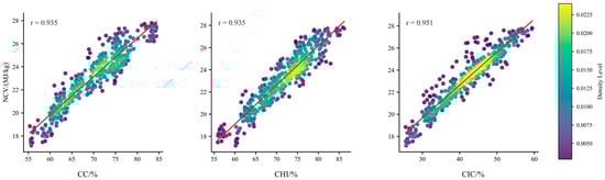
Figure 4.
Correlation between derived indicators CC, CHI, CIC and NCV.
2.3. Construction of a Calorific Value Prediction Model
2.3.1. Linear Regression Model
For the coal quality index samples in Table 2, in order to compare the linear and nonlinear modeling method for predicting calorific value, linear regression and nonlinear regression analysis conducted on the calorific value prediction process.
As can be seen from Table 1, the linear regression models can be unified and organized as follows:
In the equation, is the i-th coal quality index in Mad, Aad, VMad, FCad, Cad, Had, Nad, Sad, Oad, CC, CHI, and CIC, where i = 0 to n, and n is the maximum value of 12. When , ; is the linear coefficient of the i-th coal quality index.
If let , , , , the linear regression model in Table 1 can be uniformly expressed as a (n + 1)-dimensional hyperplane, with the specific equation as follows:
In the equation, is the linear coefficient; is the characteristic variable.
For a given proximate analysis, ultimate analysis, and calorific value sample, the set T composed of x and y can be obtained, with the specific equation as follows:
To obtain the specific form of the linear function, simply take the w and b corresponding to the minimum of the sum of the squares of the errors between the actual y values and the predicted y values. Therefore, the linear regression model for coal calorific value prediction can be converted into an optimization problem, with the specific equation as follows:
2.3.2. Nonlinear ε-SVR Model
In the process of solving the above linear regression model for calorific value, the squared loss function is used to determine the deviation between and . In fact, after normalizing the set T, if the optimal hyperplane is to be solved, only must be maximized, i.e., must be minimized [36]. Introducing the tolerance parameter , the solution of the linear regression model in Equation (7) can be converted into an optimization problem, with the specific equation as follows:
Considering that some points in set T will always appear outside hyperplane , a loss function is introduced to determine the deviation between and [37]. The specific equation is as follows:
Equation (9) can also be expressed as:
The physical meaning of this loss function is that if the distance from a point to the hyperplane is less than , the deviation between and can be considered to be 0, i.e., there is no loss. Further considering the slack variables (upper slack factor) and (lower slack factor), which have the following constraints:
The solution of Equation (11) can be further converted into an optimization problem, with the specific equations as follows:
In the formula, C is the penalty coefficient.
Generally, for convenience of solution, the Lagrange dual transformation is introduced to cancel and [38], and Equation (12) is transformed into the following formula:
In the formula, is Lagrange multiplier vector.
is also known as the ε-insensitive loss function. Its characteristic is that only points where the difference between the actual value and the predicted value is greater than ε have an effect on the model solution process. Such points are called Support Vectors [39]. Therefore, by introducing the ε-insensitive loss function , the linear regression model in Equation (7) can be transformed into a linear ε-support vector regression model, i.e., a linear ε-SVR model.
Considering that there is no strict linear relationship between the proximate analysis, ultimate analysis items, and calorific value of coal, the kernel function can be further introduced to extend Equation (13) to a nonlinear regression problem. The specific equation is as follows:
Equation (14) represents the nonlinear ε-SVR model for predicting coal calorific value. The SVR method, as a type of machine learning theory support vector machine (SVM), was first proposed by Vapnik [40]. This method introduces the kernel function to map the sample space to a higher-dimensional space, thereby achieving the goal of solving nonlinear problems using linear programming methods. It is important to note that the SVM model utilized in this study, particularly with its nonlinear radial basis function (RBF) kernel, operates by mapping data into a high-dimensional feature space to identify an optimal separating hyperplane. Consequently, the model does not yield a traditional explicit equation in the form of a linear combination of the original variables, which is a common characteristic of parametric models like linear regression. This property enhances the model’s capacity to capture complex nonlinear relationships but results in the absence of a straightforward equation form.
2.4. Ranking the Importance of Characteristic Variables in the Prediction Model
2.4.1. MIV Characteristic Variable Importance Ranking Method
For the two models used to predict coal calorific value, the linear regression model in Equation (7) and the nonlinear ε-SVR model in Equation (14), the key to determining the accuracy of the predictions is whether the input characteristic variables are selected appropriately. If all proximate analysis and ultimate analysis items are used as characteristic variables for coal calorific value prediction, not only will modeling efficiency be reduced, but model prediction accuracy may also decline significantly. Therefore, it is necessary to select the model characteristic variables. Currently, there is no clear theoretical mechanism explaining the interrelationship between coal calorific value and proximate analysis and ultimate analysis items. As a result, previous selections of characteristic variables have largely been based on correlation analysis or human experience, leading to redundant or missing model features and reducing model reliability [41,42].
This paper proposes the selection of model characteristic variables: through specific methods, variables that significantly affect calorific value are screened out as input parameters for the prediction model, while variables with less influence are eliminated. For this purpose, the mean impact value (MIV) method proposed by Dombi et al. [43] was used to select the characteristic variables for the prediction model. The main principle is as follows: select sample T to train model Ptrain; Take each characteristic variable value in the training sample T and shift it by ±10% to obtain new samples T1 and T2. Use model Ptrain to perform regression analysis on T1 and T2, yielding two regression results A1 and A2. Let E = A1 − A2 represent the change in the output result caused by the change in the characteristic variable. Further average E across the sample size to obtain the MIV. Sort the variables based on the MIVs to determine the influence of each characteristic variable on the calorific value. The flowchart of the MIV method is shown in Figure 5.
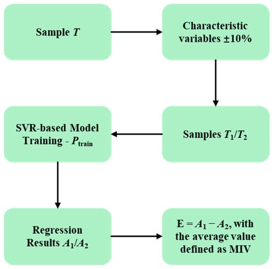
Figure 5.
Flowchart of the MIV method.
Currently, the MIV method is mainly applied in fields such as artificial neural networks [44,45,46]. This paper draws on this idea and applies it to the construction of a calorific value SVR prediction model.
2.4.2. Optimization of Model Training Parameters
Based on the MIV method, a nonlinear ε-SVR model (Equation (14)) is first used to construct the training model Ptrain. Normalize the coal original items and derived indicators in Table 2 within the range of 0 to 1 according to Equation (15) to ensure the accuracy of the prediction model. Among them, 80% of the samples are training set, which are used as input samples for model establishment T; the remaining 20% of the samples are test set, which are used as samples for model verification Ttest.
In the formula, is the scaled value of characteristic variable ; is the i-th value in characteristic variable ; is the minimum value of ; is the maximum value of .
The radial basis RBF kernel function was selected as the kernel function [47].
In the formula, is the width parameter of the kernel function.
In the nonlinear ε-SVR model (Equation (14)), parameters C and σ play an important role in the training results of the model. Therefore, C and σ need to be optimized to ensure the reliability of the trained model Ptrain. This paper employs the particle swarm optimization (PSO) algorithm to optimize C and σ [48]. During the parameter optimization process using this method, parameter searches were conducted within the ranges of C = 0.1 to 100 and σ = 0.001 to 10. The final optimized results were C = 13.798 and σ = 0.020.
2.4.3. Characteristic Variable Sorting Results
By combining the MIV algorithm with SVR, the coal original items and derived indicators in the calorific value prediction process were screened, and the MIVs of different characteristic variables and their influence weights on calorific value were calculated. The results are shown in Figure 6.
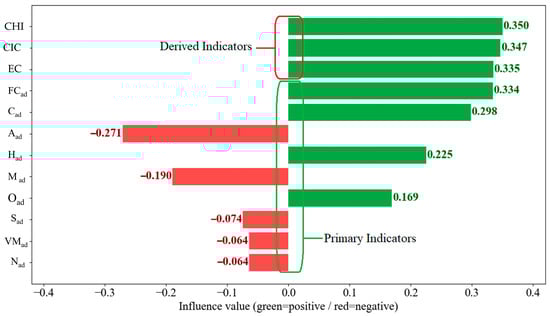
Figure 6.
MIVs and ranking of original items and derived indicators of coal.
As shown in Figure 6, the MIVs of different items vary greatly. The MIVs of items Aad, Mad, Sad, VMad, and Nad are all negative, indicating that these items are negatively correlated with calorific value. The MIVs for CHI, CC, CIC, FCad, Cad, Had, and Oad are all positive, indicating that these items are positively correlated with calorific value. Furthermore, among the coal original items, only the MIVs of the Cad, Aad, and Had items are higher than 0.200, while the MIVs of other coal original items are lower than 0.200. Meanwhile, all derived indicators such as CHI, CC, and CIC rank highly in terms of importance, and their MIVs are all higher than 0.200.
Therefore, when predicting coal calorific value, it is essential to select derived indicators as characteristic variables for the coal calorific value prediction model.
2.5. Model Development, Validation, and Software
2.5.1. Model Development
The development of both the linear regression and nonlinear SVR models followed a structured workflow. For the linear regression model (Equation (7)), the ordinary least squares method was employed to solve for the coefficients that minimize the sum of squared errors between the predicted and measured calorific values. For the more complex nonlinear ε-SVR model (Equation (14)), the development process involved several key steps:
Data Preprocessing: The entire dataset of coal quality items (Table 2) was first normalized to a [0, 1] range using Equation (15) to ensure equal weighting of all features during model training.
Data Splitting: The dataset was randomly divided into a training set (80% of samples) for model construction and a test set (the remaining 20%) for independent evaluation of the model’s predictive performance.
Kernel Selection: The RBF kernel (Equation (16)) was selected for the SVR model due to its proven effectiveness in handling complex, nonlinear relationships.
Hyperparameter Optimization: The critical hyperparameters of the SVR model, namely the penalty parameter C and the kernel width parameter σ, were optimized using the PSO algorithm. The search was conducted within the ranges of C = 0.1 to 100 and σ = 0.001 to 10, with the final optimal values determined as C = 13.798 and σ = 0.020.
2.5.2. Model Adequacy Checking
The adequacy and predictive performance of the developed models were rigorously evaluated using multiple statistical metrics calculated on the independent test set. The primary evaluation criteria were:
MAPE: To measure the average magnitude of relative prediction errors (Equation (17)).
RMSE: To quantify the absolute average prediction error, giving higher weight to large errors (Equation (18)).
R2: To assess the proportion of variance in the calorific value that is explained by the model (Equation (19)).
Furthermore, the statistical significance of the linear regression model was validated using Fisher’s F-test (Equation (20)), providing evidence that the relationship between the independent variables and the calorific value is statistically significant and not due to chance.
2.5.3. Software Information
All data preprocessing, feature selection (MIV algorithm), model development (both linear and SVR), hyperparameter optimization (PSO), and statistical analysis were performed using the Python programming language (version 3.9). The machine learning models were implemented primarily using the scikit-learn library (version 1.2.0). Numerical computations were supported by PyCharm Integrated Development Environment (version 3.1.2).
3. Results and Discussion
3.1. Evaluation Criteria for Prediction Results
The evaluation indicators for the calorific value prediction in this paper are: Mean Absolute Percentage Error (MAPE), Root Mean Square Error (RMSE), Coefficient of Determination R2, and Fisher’s criterion (F-test) [49,50,51,52]. The formulas for these calculations are as follows:
In the formula, is the measured calorific value, MJ/kg; is the predicted calorific value, MJ/kg; is the average of the measured calorific values, MJ/kg; p is the number of characteristic independent variables in the model.
3.2. Predictive Model Characteristic Variable Selection
To verify the rationality of the selected derived indicators, they needs to be evaluated. To this end, based on the nonlinear ε-SVR model in Equation (14), calorific value predictions are made for the following six combinations of characteristic variables, and the prediction results are compared:
Feature 1: Four proximate analysis items (Mad-Aad-VMad-FCad) are used as characteristic variables.
Feature 2: Five ultimate analysis items (Cad-Had-Nad-Sad-Oad) are used as characteristic variables.
Feature 3: Three derived indicators (CC-CHI-CIC) are used as characteristic variables.
Feature 4: All original items and derived indicators (Mad-Aad-VMad-FCad-Cad-Had-Nad-Sad-Oad-CC-CHI-CIC) are used as characteristic variables.
Feature 5: The top four mixed features (CC-CHI-CIC-FCad) ranked by MIV are used as characteristic variables.
Feature 6: The top five mixed features (CC-CHI-CIC-FCad-Cad) ranked by MIV are used as characteristic variables.
The PSO method was used to optimize the parameters C and σ under different characteristic variables combinations, and the calorific values were predicted. Meanwhile, to more comprehensively assess the adequacy of the regression model, this study conducted an analysis based on Fisher’s criterion (F-test) [52]. The F-test is used to validate the overall statistical significance of the model, with its null hypothesis (H0) stating that the regression coefficients of all independent variables are zero. The prediction results are shown in Table 3.
Table 3.
Calorific value prediction results by different characteristic variables combination conditions.
As shown in Table 3, when using features 1, 2, 3, and 6 to predict the calorific value of coal, the MAPE and RMSE are generally higher than those of features 4 and 5, and the R2 is generally lower than that of features 4 and 5. This indicates that when only proximate analysis, ultimate analysis, or derived indicators are used to predict the calorific value of coal, the prediction accuracy R2 is lower than 0.950, which does not meet the accuracy requirements of production practice. When using characteristic variable selection to screen out derived indicators and original items with high influence to form a mixed indicators for predicting the calorific value of coal, the prediction effect can be improved. Furthermore, when using the mixed indicators composed of the indicators in feature 5 (CC-CHI-CIC-FCad) for prediction, the prediction accuracy is not significantly different from that obtained using all indicators.
From the perspective of Fisher’s criterion (F-test), the SVM model based on Feature 5 in this study yields a remarkably high F-statistic of 1485.96, with a corresponding p-value (Prob (F-statistic)) of 1.92 × 10−261, which is far below the significance level of 0.001. This result provides extremely compelling evidence to reject the null hypothesis, indicating that the regression model constructed in this study, using CC, CHI, CIC, and FCad as input features, is highly significant. The independent variables, as a whole, possess a strong explanatory power for the dependent variable (NCV), demonstrating that the model is statistically sufficient and effective.
Compared to models using only proximate analysis (Feature 1) or ultimate analysis (Feature 2) items, the SVM model based on Feature 5 achieves a significantly higher F-value. This confirms that the combined use of derived indicators and key original items substantially enhances the model’s explanatory power and statistical significance. When compared to the model using only derived indicators (Feature 3), the introduction of fixed carbon (FCad) led to a substantial increase in the F-value from 672.41 to 1485.96. This indicates a significant synergistic effect between FC and the derived indicators, thereby optimizing model performance. Furthermore, compared to the model utilizing all indicators (Feature 4), the model presented here achieves a comparable F-value and predictive accuracy while using only 4 input variables instead of 12. This fully demonstrates that feature selection via the MIV method can ensure high model significance while substantially reducing model complexity, mitigating the risk of overfitting, and enhancing the model’s conciseness and generalizability.
Therefore, considering both prediction accuracy and model simplicity, the feature set 5 (CC-CHI-CIC-FCad) based on coal quality-derived indicators yields the best results for predicting coal calorific value. Under this condition, the MAPE, RMSE, and R2 are 1.838%, 0.544 MJ/kg, and 0.962, respectively.
In addition, when using feature 5 (CC-CHI-CIC-FCad) for NCV prediction, the relative deviation between the predicted values and the measured values is shown in Figure 7. As shown in Figure 7, when using the four indicators CC-CHI-CIC-FCad as characteristic variables for coal calorific value prediction, the relative error between the predicted values and the measured values of NCV is within ±5%, meeting the requirements of engineering practice. In summary, when using feature 5 (CC-CHI-CIC-FCad) as the input characteristic variables for the SVR method to predict NCV, the prediction accuracy is high and the model is reliable.
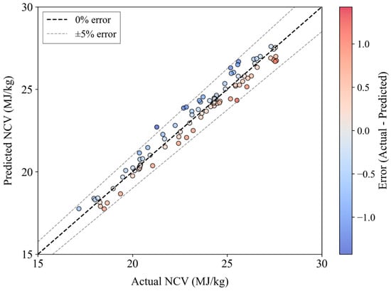
Figure 7.
Relative deviation between NCV predicted values and measured values.
3.3. Comparison of Prediction Results from Different Models
To compare the above nonlinear ε-SVR model with different linear regression models, using the data in Table 2 as the sample, the derived indicator CIC as the characteristic variable, and the linear regression method in Equation (7), a linear model for coal calorific value prediction based on derived indicators was constructed. The formulas for these calculations are as follows:
The linear correlation coefficient R2 of Equation (21) is 0.924.
Based on this, we compared the NCV prediction performance using the typical Majumder model and Chelgani model in Table 1 as reference models. The prediction accuracy is shown in Table 4, and the prediction values are compared in Figure 8.
Table 4.
Comparison of prediction accuracy of NCV by different models.
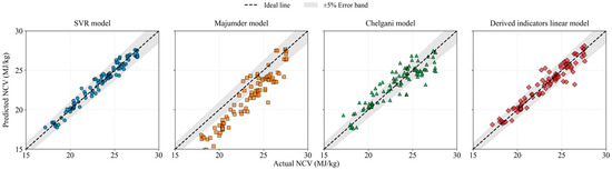
Figure 8.
Predicted values of NCV by different models.
As shown in Table 4 and Figure 8, for the process of predicting the calorific value of coal, the SVR model established in this paper has high prediction accuracy, with all prediction points evenly distributed around the 0% error line, indicating the best overall prediction performance. The Majumder model and Chelgani model both show significant deviations from the 0% error line, with the Majumder model in particular showing overall predictions that are lower than the actual measured values. The SVR model predicted lower MAPE and RMSE values and higher R2 correlation coefficients. In addition, although the accuracy of the derived indicators linear model is lower than that of the SVR model, its R2 is still above 0.90. Under conditions where accuracy requirements are not high, it can serve as an alternative model for preliminary prediction of coal calorific value.
4. Conclusions
(1) Based on 465 Chinese coal samples, this study innovatively constructed three derived indicators—CC, CHI, and CIC—for high-precision prediction of coal calorific value. By integrating nonlinear SVR with the MIV feature selection method, the study found that the linear correlation (r > 0.93) between the derived indicators and NCV was significantly stronger than that of traditional industrial and ultimate analysis items, demonstrating superior feature representation capability.
(2) The SVR prediction model established in this study demonstrated excellent performance on the test set, with the MAPE, RMSE, and R2 reaching 1.838%, 0.544 MJ/kg, and 0.962, respectively. The prediction accuracy was significantly higher than that of traditional linear models such as those proposed by Majumder and Chelgani, and the relative error of the vast majority of predicted values was controlled within ±5%. Meanwhile, the SVM model based on feature 5 yielded an F-statistic as high as 1485.96, with a corresponding p-value (Prob (F-statistic)) of 1.92 × 10−261, far below the significance level of 0.001, indicating that the model is highly statistically significant and effective. Furthermore, a simplified linear model derived from the obtained indicators was provided, offering a rapid estimation tool for field applications where lower accuracy requirements apply.
(3) The main limitation of this study lies in the fact that all samples were sourced from China; the model’s generalizability to regions with different coal-forming geological backgrounds requires further validation. Future work will focus on expanding the sample set to include global sources to verify the model’s generalizability and promote its integration into industrial online analysis systems.
Author Contributions
Conceptualization, X.W. and D.L.; methodology, X.W., D.L., Y.J. and Y.Y.; software, Y.J. and Y.Y.; validation, Y.J. and Y.Y.; formal analysis, X.W.; investigation, X.W. and D.L.; resources, Z.C.; data curation, X.W. and Y.J.; writing—original draft preparation, X.W.; writing—review and editing, D.L.; visualization, Y.J.; supervision, D.L.; project administration, D.L. and Z.C.; funding acquisition, Z.C. All authors have read and agreed to the published version of the manuscript.
Funding
This work was supported by the Key Research and Development and Achievement Transformation Plan Project of Inner Mongolia Autonomous Region [grant number 2025KJHZ0004], the First-Class Discipline Research Special Project of Inner Mongolia Autonomous Region [grant number YLXKZX-NKD-054], the Natural Science Foundation of Inner Mongolia of China [grant number 2023MS05007], and the Basic Research Business Foundation of Administrated Universities of Inner Mongolia of China [grant number 2023QNJS100], and the Inner Mongolia Natural Science Foundation [grant number 2023MS05010].
Data Availability Statement
The dataset of proximate analysis, ultimate analysis, and net calorific value for the 465 coal samples supporting this study have been deposited in the Figshare repository [https://doi.org/10.6084/m9.figshare.30391066].
Conflicts of Interest
The authors declare no competing financial interest.
Abbreviations
| Abbreviation/Symbol | Full Name/Explanation |
| ANN | Artificial Neural Network |
| GCV | Gross Calorific Value (synonymous with HHV) |
| GPR | Gaussian Process Regression |
| MAPE | Mean Absolute Percentage Error |
| MIV | Mean Impact Value |
| MLR | Multiple Linear Regression |
| MVRA | Multiple Variable Regression Analysis |
| NCV | Net Calorific Value |
| PSO | Particle Swarm Optimization |
| R2 | Coefficient of Determination |
| RBF | Radial Basis Function (Kernel) |
| RMSE | Root Mean Square Error |
| SVM | Support Vector Machine |
| SVR | Support Vector Regression |
| Nomenclature | Full Name/Explanation |
| Aad | Ash content (proximate analysis) |
| Cad | Carbon content (ultimate analysis) |
| CC | Combustible Content (derived indicator) |
| CHI | Carbon-Hydrogen Index(derived indicator) |
| CIC | Carbon in Combustibles (derived indicator) |
| FCad | Fixed Carbon (proximate analysis) |
| Had | Hydrogen content (ultimate analysis) |
| Mad | Moisture content (proximate analysis) |
| Nad | Nitrogen content (ultimate analysis) |
| Oad | Oxygen content (ultimate analysis) |
| Sad | Sulfur content (ultimate analysis) |
| VMad | Volatile Matter (proximate analysis) |
| a(*) | Lagrange multiplier vector |
| C | Penalty coefficient (SVR model) |
| p | Number of characteristic independent variables in the model |
| r | Pearson correlation coefficients |
| w | Linear coefficient |
| x | Characteristic variable. |
| I-th value in characteristic variable | |
| Minimum value of | |
| Maximum value of | |
| Scaled value of characteristic variable | |
| Received basis moisture content of the coal sample | |
| ε-insensitive loss function | |
| Measured calorific value | |
| Predicted calorific value | |
| Average of the measured calorific values | |
| Upper slack factor | |
| Lower slack factor | |
| Greek symbols | Full Name/Explanation |
| σ | Width parameter of the RBF kernel function (sigma) |
| ε | Tolerance parameter in ε-SVR (epsilon) |
| Width parameter of the kernel function | |
| Subscripts | Full Name/Explanation |
| ad | Air-dried basis |
| ar | As-received basis |
| daf | Dry ash-free basis |
References
- Erdoğan, S. LHV and HHV prediction model using regression analysis with the help of bond energies for biodiesel. Fuel 2021, 301, 121065. [Google Scholar] [CrossRef]
- Yerel, S.; Ersen, T. Prediction of the Calorific Value of Coal Deposit Using Linear Regression Analysis. Energy Sources Part A-Recovery Util. Environ. Eff. 2013, 35, 976–980. [Google Scholar] [CrossRef]
- Heriawan, M.N.; Koike, K. Identifying spatial heterogeneity of coal resource quality in a multilayer coal deposit by multivariate geostatistics. Int. J. Coal Geol. 2008, 73, 307–330. [Google Scholar] [CrossRef]
- Bech, N.; Jensen, P.A.; Dam-Johansen, K. Determining the elemental composition of fuels by bomb calorimetry and the inverse correlation of HHV with elemental composition. Biomass Bioenergy 2009, 33, 534–537. [Google Scholar] [CrossRef]
- Mason, D.M.; Gandhi, K.N. Formulas for calculating the calorific value of coal and coal chars: Development, tests, and uses. Fuel Process. Technol. 1983, 7, 11–22. [Google Scholar] [CrossRef]
- Given, P.H.; Weldon, D.; Zoeller, J.H. Calculation of calorific values of coals from ultimate analyses: Theoretical basis and geochemical implications. Fuel 1986, 65, 849–854. [Google Scholar] [CrossRef]
- Küçükbayrak, S.; Dürüs, B.; Meríçboyu, A.E.; Kadioglu, E. Estimation of calorific values of Turkish lignites. Fuel 1991, 70, 979–981. [Google Scholar] [CrossRef]
- Majumder, A.K.; Jain, R.; Banerjee, P.; Barnwal, J.P. Development of a new proximate analysis based correlation to predict calorific value of coal. Fuel 2008, 87, 3077–3081. [Google Scholar] [CrossRef]
- Chelgani, S.C.; Makaremi, S. Explaining the relationship between common coal analyses and Afghan coal parameters using statistical modeling methods. Fuel Process. Technol. 2013, 110, 79–85. [Google Scholar] [CrossRef]
- Akhtar, J.; Naseer, S.; Munir, S. Linear regression-based correlations for estimation of high heating values of Pakistani lignite coals. Energy Sources Part A Recovery Util. Environ. Eff. 2017, 39, 1063–1070. [Google Scholar] [CrossRef]
- Mesroghli, S.; Jorjani, E.; Chelgani, S.C. Estimation of gross calorific value based on coal analysis using regression and artificial neural networks. Int. J. Coal Geol. 2009, 79, 49–54. [Google Scholar] [CrossRef]
- Patel, S.U.; Kumar, B.J.; Badhe, Y.P.; Sharma, B.K.; Saha, S.; Biswas, S.; Chaudhury, A.; Tambe, S.S.; Kulkarni, B.D. Estimation of gross calorific value of coals using artificial neural networks. Fuel 2007, 86, 334–344. [Google Scholar] [CrossRef]
- Khandelwal, M.; Singh, T.N. Prediction of macerals contents of Indian coals from proximate and ultimate analyses using artificial neural networks. Fuel 2010, 89, 1101–1109. [Google Scholar] [CrossRef]
- Mondal, C.; Pandey, A.; Pal, S.K.; Samanta, B.; Dutta, D. Prediction of gross calorific value as a function of proximate parameters for Jharia and Raniganj coal using machine learning based regression methods. Int. J. Coal Prep. Util. 2022, 42, 3763–3776. [Google Scholar] [CrossRef]
- Akkaya, A.V.; Cetin, B. Formulating a novel combined equation for coal calorific value estimation by group method data handling type neural network. Energy Sources Part A-Recovery Util. Environ. Eff. 2024, 46, 15492–15505. [Google Scholar] [CrossRef]
- Kavsek, D.; Bednarova, A.; Biro, M.; Kranvogl, R.; Voncina, D.B.; Beinrohr, E. Characterization of Slovenian coal and estimation of coal heating value based on proximate analysis using regression and artificial neural networks. Cent. Eur. J. Chem. 2013, 11, 1481–1491. [Google Scholar]
- Tan, P.; Zhang, C.; Xia, J.; Fang, Q.Y.; Chen, G. Estimation of higher heating value of coal based on proximate analysis using support vector regression. Fuel Process. Technol. 2015, 138, 298–304. [Google Scholar] [CrossRef]
- Akkaya, A.V. Coal higher heating value prediction using constituents of proximate analysis: Gaussian process regression model. Int. J. Coal Prep. Util. 2022, 42, 1952–1967. [Google Scholar] [CrossRef]
- Li, L.J.; Su, H.Y.; Chu, J. Modeling of Isomerization of C8 Aromatics by Online Least Squares Support Vector Machine. Chin. J. Chem. Eng. 2009, 17, 437–444. [Google Scholar] [CrossRef]
- Chen, J.; He, Y.; Liang, Y.; Wang, W.; Duan, X. Estimation of gross calorific value of coal based on the cubist regression model. Sci. Rep. 2024, 14, 23176. [Google Scholar] [CrossRef] [PubMed]
- Sciazko, M. Rank-dependent formation enthalpy of coal. Fuel 2013, 114, 2–9. [Google Scholar] [CrossRef]
- Channiwala, S.A.; Parikh, P.P. A unified correlation for estimating HHV of solid, liquid and gaseous fuels. Fuel 2002, 81, 1051–1063. [Google Scholar] [CrossRef]
- Selvig, W.A.; Gibson, I.H. Calorifc value of coal. In Chemistry of Coal Utilization; Lowry, H.H., Ed.; Wiley: New York, NY, USA, 1945; Volume 1, p. 139. [Google Scholar]
- Strache, H.; Lant, R. Kohlenchemie; Akademische Verlags-Gesellschaft: Leipzig, Germany, 1924; p. 476. [Google Scholar]
- Wilson, D.L. Prediction of heat of combustion of solid wastes from ultimate analysis. Environ. Sci. Technol. 1972, 6, 1119–1121. [Google Scholar] [CrossRef]
- Speight, J.G. Handbook of Coal Analysis; John Wiley & Sons: Hoboken, NJ, USA, 2015; pp. 144–169. [Google Scholar]
- Parikh, J.; Channiwala, S.A.; Ghosal, G.K. A correlation for calculating HHV from proximate analysis of solid fuels. Fuel 2005, 84, 487–494. [Google Scholar] [CrossRef]
- Chelgani, S.C.; Mesroghli, S.; Hower, J.C. Simultaneous prediction of coal rank parameters based on ultimate analysis using regression and artificial neural network. Int. J. Coal Geol. 2010, 83, 31–34. [Google Scholar] [CrossRef]
- Kowalik-Klimczak, A.; Lozynska, M.; Zycki, M.; Wozniak, B. The Effect of the Pyrolysis Temperature of a Leather-Textile Mixture from Post-Consumer Footwear on the Composition and Structure of Carbonised Materials. Materials 2024, 17, 5649. [Google Scholar] [CrossRef] [PubMed]
- Ai, Z.P.; Xiao, Z.F.; Liu, M.H.; Zhou, L.Q.; Yang, L.J.; Huang, Y.J.; Xiong, Q.Q.; Li, T.; Liu, Y.H.; Xiao, H.W.; et al. Evaluation of innovative drying technologies in Gardenia jasminoides Ellis drying considering product quality and drying efficiency. Food Chem.-X 2024, 24, 102052. [Google Scholar] [CrossRef]
- Wang, Y.C.; Liu, Z.L.; Chen, F.; Xiong, X.C. MSA-Net: A Precise and Robust Model for Predicting the Carbon Content on an As-Received Basis of Coal. Sensors 2024, 24, 4607. [Google Scholar] [CrossRef] [PubMed]
- Yu, S.; Kim, H.; Park, J.; Lee, Y.; Park, Y.K.; Ryu, C. Relationship between torrefaction severity, product properties, and pyrolysis characteristics of various biomass. Int. J. Energy Res. 2022, 46, 8145–8157. [Google Scholar] [CrossRef]
- Forman, J.L.; Sorensen, M. The pearson diffusions: A class of statistically tractable diffusion processes. Scand. J. Stat. 2008, 35, 438–465. [Google Scholar] [CrossRef]
- Bishara, A.J.; Hittner, J.B. Testing the significance of a correlation with nonnormal data: Comparison of Pearson, Spearman, transformation, and resampling approaches. Psychol. Methods 2012, 17, 399–417. [Google Scholar] [CrossRef] [PubMed]
- Alekhnovich, A.N. Estimating the Heating Value of Coals Based on the Composition. Power Technol. Eng. 2020, 53, 724–730. [Google Scholar] [CrossRef]
- Vapnik, V.N.; Chervonenkis, A.Y. On the Uniform Convergence of Relative Frequencies of Events to Their Probabilities. Theory Probab. Appl. 1971, 16, 264–280. [Google Scholar] [CrossRef]
- Kozan, E. A New Estimation Approach in Machine Learning Regression Model. Int. J. Ind. Eng. Theory Appl. Pract. 2024, 31, 830–837. [Google Scholar]
- Smola, A.J.; Schölkopf, B. A tutorial on support vector regression. Stat. Comput. 2004, 14, 199–222. [Google Scholar] [CrossRef]
- Luo, H.C.; Zhou, P.J.; Cui, J.Y.; Wang, Y.; Zheng, H.S.; Wang, Y.T. Energy performance prediction of centrifugal pumps based on adaptive support vector regression. Eng. Appl. Artif. Intell. 2025, 145, 110247. [Google Scholar] [CrossRef]
- Vapnik, V.; Golowich, S.E.; Smola, A. Support vector method for function approximation, regression estimation and signal processing. In Proceedings of the 10th International Conference on Neural Information Processing Systems, Denver, CO, USA, 3–5 December 1996; MIT Press: Denver, CO, USA, 1996; pp. 281–287. [Google Scholar]
- Chelgani, S.C.; Shahbazi, B.; Hadavandi, E. Support vector regression modeling of coal flotation based on variable importance measurements by mutual information method. Measurement 2018, 114, 102–108. [Google Scholar] [CrossRef]
- Xu, S.; Lu, B.; Baldea, M.; Edgar, T.F.; Nixon, M. An improved variable selection method for support vector regression in NIR spectral modeling. J. Process Control 2018, 67, 83–93. [Google Scholar] [CrossRef]
- Dombi, G.W.; Nandi, P.; Saxe, J.M.; Ledgerwood, A.M.; Lucas, C.E. Prediction of rib fracture injury outcome by an artificial neural network. J. Trauma 1995, 39, 915–921. [Google Scholar] [CrossRef]
- Chen, Z.; Jia, K.; Xiao, C.; Wei, D.; Zhao, X.; Lan, J.; Wei, X.; Yao, Y.; Wang, B.; Sun, Y.; et al. Leaf Area Index Estimation Algorithm for GF-5 Hyperspectral Data Based on Different Feature Selection and Machine Learning Methods. Remote Sens. 2020, 12, 2110. [Google Scholar] [CrossRef]
- Liu, Z.; Yang, B.; Ma, C.; Wang, S.; Yang, Y. Thermal error modeling of gear hobbing machine based on IGWO-GRNN. Int. J. Adv. Manuf. Technol. 2020, 106, 5001–5016. [Google Scholar] [CrossRef]
- Zheng, J.; Lan, Q.; Zhang, X.; Kainz, W.; Chen, J. Prediction of MRI RF Exposure for Implantable Plate Devices Using Artificial Neural Network. IEEE Trans. Electromagn. Compat. 2020, 62, 673–681. [Google Scholar] [CrossRef]
- Huang, Y.; Lu, T.; Ding, X.; Gu, N. Campus Building Energy Usage Analysis and Prediction: A SVR Approach Based on Multi-scale RBF Kernels. In Proceedings of the Human Centered Computing: First International Conference, HCC 2014, Phnom Penh, Cambodia, 27–29 November 2014; Revised Selected Papers. Springer: Phnom Penh, Cambodia, 2014; pp. 441–452. [Google Scholar]
- Mahapatra, A.K.; Panda, N.; Mahapatra, M.; Jena, T.; Mohanty, A.K. A fast-flying particle swarm optimization for resolving constrained optimization and feature selection problems. Clust. Comput.-J. Netw. Softw. Tools Appl. 2025, 28, 91. [Google Scholar] [CrossRef]
- De Myttenaere, A.; Golden, B.; Le Grand, B.; Rossi, F. Mean Absolute Percentage Error for regression models. Neurocomputing 2016, 192, 38–48. [Google Scholar] [CrossRef]
- Taraji, M.; Haddad, P.R.; Amos, R.I.J.; Talebi, M.; Szucs, R.; Dolan, J.W.; Pohl, C.A. Error measures in quantitative structure-retention relationships studies. J. Chromatogr. A 2017, 1524, 298–302. [Google Scholar] [CrossRef] [PubMed]
- Xu, X.B.; Du, H.; Lian, Z.W. Discussion on regression analysis with small determination coefficient in human-environment researches. Indoor Air 2022, 32, 13117. [Google Scholar] [CrossRef]
- Pyshyev, S.; Prysiazhnyi, Y.; Bilushchak, H.; Korchak, B.; Pochapska, I.; Yavorskyi, O. Creation of experimental-statistical and kinetic models of the coumarone-indene-carbazole resin production process. Results Eng. 2025, 25, 103689. [Google Scholar] [CrossRef]


Disclaimer/Publisher’s Note: The statements, opinions and data contained in all publications are solely those of the individual author(s) and contributor(s) and not of MDPI and/or the editor(s). MDPI and/or the editor(s) disclaim responsibility for any injury to people or property resulting from any ideas, methods, instructions or products referred to in the content. |
© 2025 by the authors. Licensee MDPI, Basel, Switzerland. This article is an open access article distributed under the terms and conditions of the Creative Commons Attribution (CC BY) license (https://creativecommons.org/licenses/by/4.0/).