Abstract
In response to the limitations of traditional single-signal approaches, which fail to comprehensively reflect fault conditions, and the difficulties of existing feature extraction methods in capturing subtle fault patterns in transformer fault diagnosis, this paper proposes an innovative fault diagnosis methodology. Initially, to address common severe faults in excitation transformers, Principal Component Analysis (PCA) is applied to reduce the dimensionality of multi-source feature data, effectively eliminating redundant information. Subsequently, to mitigate the impact of non-stationary noise interference in voiceprint signals, a Deep Belief Network (DBN) optimized using the Hunter–Prey Optimization (HPO) algorithm is employed to automatically extract deep features highly correlated with faults, thus enabling the detection of complex, subtle fault patterns. For temperature and electrical parameter signals, which contain abundant time-domain information, the Random Forest algorithm is utilized to evaluate and select the most relevant time-domain statistics. Nonlinear dimensionality reduction is then performed using an autoencoder to further reduce redundant features. Finally, a multi-classifier model based on Adaptive Boosting with Support Vector Machine (Adaboost-SVM) is constructed to fuse multi-source heterogeneous information. By incorporating a pseudo-label self-training strategy and integrating a working condition awareness mechanism, the model effectively analyzes feature distribution differences across varying operational conditions, selecting potential unseen condition samples for training. This approach enhances the model’s adaptability and stability, enabling real-time fault diagnosis. Experimental results demonstrate that the proposed method achieves an overall accuracy of 96.89% in excitation transformer fault diagnosis, outperforming traditional models such as SVM, Extreme Gradient Boosting with Support Vector Machine (XGBoost-SVM), and Convolutional Neural Network (CNN). The method proves to be highly practical and generalizable, significantly improving fault diagnosis accuracy.
1. Introduction
The generator excitation system provides excitation current to the generator, playing a crucial role in maintaining its normal and stable operation [1]. As a three-phase alternating current excitation power device in large generator excitation systems, the excitation transformer is exposed to the combined effects of alternating voltage and pulse voltage during operation, resulting in a complex insulation aging process. Furthermore, due to prolonged high-load operation and harsh environmental conditions, excitation transformers are susceptible to various faults, including partial discharge [2], grounding faults [3], and direct current bias magnetization [4]. The safe and stable operation of the excitation transformer is essential for the reliability of the self-excitation system and is a prerequisite for ensuring safe electricity production and full-capacity generation in power plants. Therefore, real-time monitoring and precise fault diagnosis of excitation transformers are critical for ensuring the safe operation of the unit and facilitating planned maintenance.
Existing transformer fault diagnosis methods can be broadly categorized into offline testing and online monitoring techniques [5]. Offline testing methods include low-voltage pulse testing, short-circuit impedance testing, and frequency response analysis [6,7]. While these methods are well-established, they require the transformer to be shut down for implementation, which disrupts production schedules and incurs high labor costs. In contrast, online monitoring involves the real-time collection of data on parameters such as vibration [8], partial discharge [9,10], electrical characteristics [11], and dissolved gases in oil [12], all of which provide insights into the transformer’s operational status and potential faults. However, for dry-type transformers, the absence of cooling oil data limits the development of online fault diagnosis techniques. Additionally, in power plant monitoring systems, the diversity of data types and their often nonlinear interdependencies present challenges. Effectively extracting valuable information from the large volume of operational data, while mitigating issues such as the incompleteness of single-signal diagnostics and interference from environmental noise [13], is crucial for reducing both misdiagnoses and missed diagnoses of faults.
Transformers typically exhibit changes in the electromagnetic field under fault conditions [14], which in turn influence the vibration and acoustic characteristics of the components. Vibration and voiceprint signals contain rich information regarding the equipment’s operational status, and by analyzing these signals, effective fault diagnosis of transformers can be achieved. In recent years, extensive research has been conducted both domestically and internationally on transformer condition monitoring techniques based on vibration and voiceprint signals. Compared to vibration signals, voiceprint signals offer several advantages, including non-contact measurement, making them particularly promising for application. Zhang et al. [15] proposed a method for estimating the internal aging degree of transformers by collecting acoustic signals from both the high and low voltage sides and combining these signals with a backpropagation neural network. Li et al. [16] addressed the challenge of diagnosing faults in converter transformers by proposing a fault diagnosis method that integrates multi-strategy enhanced Mel-Frequency Cepstral Coefficients (MFCC) feature extraction with Improved Hunter–Prey Optimization-optimized (IHPO-optimized) time convolution networks, thereby improving feature representation and model recognition capabilities. Yu et al. [17] explored the voiceprint features of internal vibration sound signals in power transformers under various operating conditions and developed an automatic, non-invasive condition monitoring and fault diagnosis system based on acoustic characteristics. This system is capable of rapidly distinguishing fault operating conditions across different noise environments and diagnosing six typical faults, as well as mixed faults, in power transformers.
However, under complex operating conditions, fault diagnosis methods based on single signals still face limitations in terms of identification capability and stability. Additionally, the types and degrees of interference factors in on-site operating environments are highly uncertain. To address these challenges, multi-sensor information fusion technology has gained widespread application in fault diagnosis in recent years, achieving significant results in areas such as dissolved gas detection in transformer oil. For instance, Gong et al. [18] proposed a novel multi-source information fusion strategy that combines a hierarchical vision transformer with a wavelet time-frequency architecture. By extracting and integrating features from vibration and current signals, this method enhances the stability of diagnostic performance. Cui et al. [19] introduced an intelligent fault diagnosis method based on multi-source data fusion and correlation analysis, utilizing an improved entropy-weighted method to fuse and predict data related to the load rate of dissolved gases in transformers, upper oil temperature, winding temperature, and the melting index of dissolved gas components. Hou et al. [20] developed a fault diagnosis method based on transformer information fusion technology, which combines a probabilistic extreme learning machine with an improved Dempster–Shafer (D-S) evidence theory. This method applies the enhanced D-S evidence theory algorithm to fuse multiple evidence bodies, enabling comprehensive transformer diagnostics. Tests on real fault data have demonstrated that this approach significantly improves the accuracy of diagnostic results.
Feature extraction, as a core element of fault diagnosis, aims to transform raw monitoring signals into feature information that possesses clear physical meaning or strong discriminatory power. Common signal processing methods currently include Fourier decomposition, wavelet analysis, and others. Zhu et al. [21] extracted time-frequency features of azimuth signals using Wavelet Packet Transform (WPT), forming a time-frequency feature matrix. The features of the matrix obtained by WPT were then further processed, with irrelevant features removed and fault-sensitive features retained. The resulting feature matrix was used as input to a classifier for bearing fault diagnosis. However, traditional signal feature extraction methods are heavily reliant on manual expertise, making it challenging to effectively capture nonlinear features. Additionally, they are sensitive to noise, limiting their adaptability and robustness under complex operating conditions. In contrast, deep learning methods can automatically learn multi-level, high-dimensional abstract features directly from raw data without manual design. This characteristic makes deep learning particularly suitable for complex nonlinear systems, contributing to its widespread application in feature extraction. Xue et al. [22] constructed multiple independent network structures in the time, frequency, and time-frequency domains. One network was used for supervised feature fusion, while other networks autonomously performed feature extraction through multiple Inception layers and convolutional layers. To support the extraction of key features across multiple fusion layers in different transformation domains, Xue et al. introduced multiple fusion nodes between the layers of various feature extraction networks and the feature summary network. Experimental results demonstrated that multi-transformation domain feature fusion significantly enhanced performance, surpassing the results of single-domain fusion methods.
To address the limitations in the current fault diagnosis methods for excitation transformers, this paper proposes a fault classification approach that leverages the Hunter–Prey Optimization (HPO) algorithm for optimizing DBN and multi-source heterogeneous information fusion, integrating advanced machine learning and signal processing techniques. In this method, HPO is employed to optimize the hyperparameters of the Deep Belief Network (DBN) network, allowing it to automatically extract deep features from voiceprint signals that are closely correlated with faults and effectively capture the complex patterns of subtle faults. Furthermore, by incorporating multi-source monitoring information, such as temperature and electrical parameters, and introducing a working condition awareness indicator, a classification model based on Adaboost-SVM is developed to perform semi-supervised fault diagnosis for excitation transformers.
2. Feature Extraction for Excitation Transformers
2.1. Feature Parameter Selection Based on Principal Component Analysis (PCA)
The excitation transformer studied in this paper features a combined three-phase dry-type structure, with the main components consisting of windings and a core. The windings are manufactured using an epoxy resin encapsulation process, which enhances their resistance to deformation. As auxiliary equipment for synchronous generators, the output current from the excitation transformer is rectified by a thyristor rectifier to provide a DC excitation current to the generator. Consequently, the winding current of the excitation transformer contains high-order harmonic non-sinusoidal components. In addition to the fundamental losses, this results in additional losses, such as eddy current losses in the windings, connection line losses, stray losses in structural components, and an increase in winding temperature. Furthermore, the thyristor rectifier generates a pulse voltage during its on/off control process, which, when superimposed on the pulsating AC voltage, affects the low-voltage winding of the excitation transformer [23,24]. To investigate various fault types, this paper establishes a finite element simulation model of the excitation transformer based on fault occurrence probability and severity, simulating four typical abnormal states: partial discharge, DC bias magnetization, component loosening, and multi-point grounding of the core. The DC component generated by the thyristor rectifier can induce DC bias in the excitation transformer. Furthermore, the excitation transformer’s maximum operating temperature can reach 150 °C, which can lead to local insulation degradation and facilitate the occurrence and progression of partial discharge. Additionally, multi-point grounding faults in dry-type transformer cores, often caused by manufacturing defects or improper construction, are the most frequent type of core electrical fault, with potentially severe consequences. Component loosening faults also occur periodically due to thermal stress and mechanical shocks during operation. Given the probability and severity of these faults, this paper establishes a finite element simulation model for the excitation transformer, addressing four common faults: partial discharge, component loosening, and the significant impacts of DC bias and multi-point grounding in the core, in order to conduct fault diagnosis research.
During the four fault simulation scenarios, five typical operating states and conditions were established: no-load rated voltage, no-load at 90% of rated voltage, no-load at 80% of rated voltage, load at 75% of rated voltage, and load at 80% of rated voltage. A series of simulation data were generated under these conditions. Based on the variations observed in the electromagnetic, thermal, and voiceprint characteristics, six key parameters were statistically analyzed: the leakage magnetic distortion amplitude (LM), defined as the maximum axial leakage magnetic variation at the 1/4, mid, and 3/4 heights of the winding; the effective value of power loss (PL); the hot-spot temperature of the winding (HT); the amplitude of the time-domain voiceprint signal (VT); the dominant frequency ratio in the frequency-domain voiceprint signal (VF); and the effective value of the core ground current (CC). To minimize noise and eliminate redundant information, Principal Component Analysis (PCA) is applied for dimensionality reduction on the aforementioned features [25,26]. After performing a linear transformation of the original feature data, the variance information of each principal component is displayed in Figure 1. To balance information fidelity and noise, we set the variance threshold at 85%. As shown in the figure, the cumulative variance of the first three principal components exceeds 85%, indicating that these components capture most of the fault characteristic information. For each fault type, the first principal component provides the strongest feature representation. However, PCA measures variance rather than separability. Therefore, retaining the first three principal components not only satisfies the ≥85% variance criterion but also ensures a consistent feature dimension across different operating conditions, facilitating model training and comparison. Additionally, this approach preserves structured information beyond PC1 with minimal additional dimensional cost.
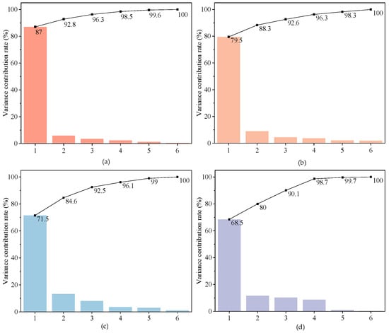
Figure 1.
Principal component variance information chart. (a) Principal components of partial discharge; (b) Principal components of DC magnetic bias; (c) Principal components of component loosening; (d) Principal components of multi-point core grounding.
The principal component coefficients of the feature parameters under different fault conditions are presented in Table 1. Based on the directionality of the maximum coefficients, it can be inferred that the power loss signal, winding temperature signal, voiceprint signal, and core grounding current signal are critical features for characterizing the operational status of the excitation transformer.

Table 1.
Principal component coefficients of feature parameters.
In addition to considering the contribution of the features, it is essential to assess their discriminability within the samples. Therefore, this paper introduces the Laplacian Score (LS) metric to evaluate the remaining features. The resulting feature scores for different types of features are presented in Figure 2.
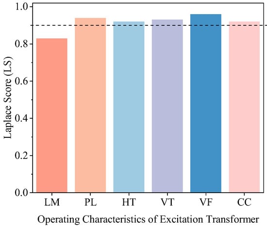
Figure 2.
Feature scoring results.
The results indicate that the Laplacian scores for the power loss signal, winding temperature signal, voiceprint signal, and core grounding current signal all exceed 0.9, suggesting that their feature data exhibit strong clustering ability.
2.2. Feature Extraction Based on the HPO-DBN Model
This paper constructs the HPO-DBN model, which directly extracts deep features related to faults from the raw voiceprint signals of the excitation transformer, effectively identifying subtle fault patterns. DBN (Deep Belief Network) is a multi-layer neural network composed of stacked Restricted Boltzmann Machines (RBMs). It utilizes an unsupervised layer-by-layer training mechanism, enabling it to learn complex signal mapping functions characterized by high-dimensional nonlinearity, non-stationary behavior, and weak state signals. The output of each RBM layer serves as the input for the subsequent layer, facilitating the extraction of deeper features at each level. Ultimately, the performance of the DBN is enhanced through supervised fine-tuning in the reverse direction. However, the performance of the DBN is heavily dependent on hyperparameters such as the number of RBM layers, the number of neurons in each RBM layer, and the learning rate. Accurately determining these parameters through experience is challenging, and manual tuning is both inefficient and unstable. To address this, this paper introduces the HPO algorithm, proposed by Naruei et al. in [27], which automates the optimization and fine-tuning of DBN parameters. By simulating the behavior of hunters tracking prey, this algorithm demonstrates strong global search capabilities. The specific steps for applying HPO in DBN parameter optimization are outlined in Table 2.
Table 2.
HPO-DBN Pseudocode.
The structural diagram illustrating the application of the Hunter–Prey Optimization (HPO) algorithm to optimize the DBN parameters is presented in Figure 3.
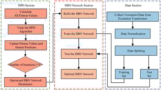
Figure 3.
The structure diagram of the HPO-DBN.
2.3. Feature Extraction Based on Random Forest and Autoencoder
The time-domain statistical features of the temperature and electrical parameter signals were extracted using Tsfresh version 0.20.3. Tsfresh is a Python-based tool for time-series feature extraction that can automatically extract over 50 types of time-domain statistical features, such as mean, standard deviation, peak value, and others [28]. Table 3 presents a selection of the time-domain statistical quantities of the temperature and electrical signals extracted using the Tsfresh library.
Table 3.
Types of time-domain statistical quantities for temperature and electrical signals.
When high-dimensional time-domain statistical features are directly input into a classification model for fault diagnosis, it often results in low diagnostic accuracy. Additionally, the overfitting of irrelevant features during model training can reduce training efficiency, thereby diminishing the reliability of fault diagnosis. To address these issues, this paper first employs Random Forest to rank the importance of the features, enabling an initial dimensionality reduction of temperature and electrical signal features. After selecting features based on their importance, the resulting feature set may still contain highly correlated redundant features. Excessive redundancy can weaken the significance of other features in the model’s decision-making process, ultimately reducing classification accuracy. To mitigate this, an autoencoder is further introduced to perform nonlinear dimensionality reduction on the selected important features, aiming to derive a low-dimensional, non-redundant feature set for temperature and electrical signals. The specific feature extraction process is illustrated in Figure 4.
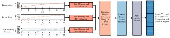
Figure 4.
Schematic of feature extraction based on random forest and autoencoder.
3. Fault Diagnosis Framework Based on Multi-Source Heterogeneous Information Fusion
Due to differences in sampling frequency and response time among the excitation transformer voiceprint data, temperature data, and electrical parameter data, as well as the potential data processing delays during classifier computation, it is essential to partition the heterogeneous signals collected from multiple sensors into windows. This partitioning ensures time synchronization of different signal types within the same time window, thereby enhancing the timeliness of fault diagnosis. Specifically, for the voiceprint signal, a 1 s time window with a 1 s sliding step is employed, and down sampling is performed with an interval of 10 to generate several sub-samples. For the temperature and electrical signals, a 10 min time window with a 1 s sliding step is used, similarly partitioned into multiple sub-samples. Given the high dimensionality and large volume of the collected data, practical applications may encounter issues such as packet loss or data instability, leading to missing values and anomalies. These challenges can adversely affect model training and diagnostic accuracy. To address these issues, this study employs the Isolation Forest (IF) algorithm to detect outliers at the window level. Missing values are then imputed using the median substitution method, completing the data cleaning process. Finally, the data is normalized using the Z-score method.
Furthermore, considering the complex and variable operating conditions encountered in the actual operation of excitation transformers, traditional semi-supervised learning methods often fail to fully account for the differences in the distribution of unlabeled samples across these conditions. As a result, the model may overfit the observed conditions, leading to performance degradation when applied to new conditions. To address this challenge, this paper introduces a working condition awareness mechanism. By utilizing distribution distance information in the feature space, the mechanism selects unlabeled samples that significantly differ from the labeled samples and incorporates them into the training set. This approach enhances the model’s adaptability and generalization ability to diverse operating conditions.
The Mahalanobis distance between the center of the unlabeled samples and the labeled samples is calculated using Equation (1) [29] as an indicator of operating condition differences. This distance is then combined with confidence and disparity thresholds for dual filtering, which facilitates the construction of a pseudo-label dataset.
In the equation, Dj represents the computed Mahalanobis distance, xi denotes the unlabeled sample, where i = 1, 2, …, N, c is the center of all labeled samples, and S is the covariance matrix of the training samples.
Finally, to meet the real-time and fast requirements of excitation transformer fault diagnosis, a Support Vector Machine (SVM) is selected as the base classifier for Adaboost [30], and a fault diagnosis model is constructed. Given a sample dataset containing n sets of training data K = {(x1, y1), …, (xn, yn)}, where xn represents the n-th feature vector and yn is its corresponding label, taking values of −1 or 1. The weight of the i-th sample is denoted by ai, with the initial sample weight set as ai = 1/n. The number of iterations is denoted by m.
The initial feature parameters are input into the SVM to obtain the t-th initial weak classifier as follows:
Calculate the classification error Eeer of the weak classifier as follows:
Adjust the weight coefficient at of the t-th sample based on its classification error as follows:
Reallocate the weights of each sample and adjust the sample distribution based on the magnitude of the weight coefficients as follows:
In the formula, Ct is the generalization coefficient. If the distribution of a certain sample is the same as the previous one, exit the loop; otherwise, continue the loop.
The resulting combined strong classifier is
In the formula, sign represents the sign function, and n denotes the number of weak classifiers.
The overall framework is illustrated in Figure 5.
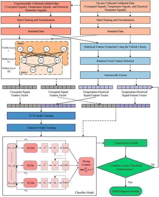
Figure 5.
Fault diagnosis framework of excitation transformer based on Adaboost-SVM. The solid line in the figure represents the experimentally collected labeled data, while the dashed line represents the on-site collected unlabeled data.
4. Model Evaluation
4.1. Dataset Acquisition
The experimental subject of this study is a three-phase modular, resin-cast, F-class insulated, dry-type excitation transformer with a rated capacity of 3200 kVA and a primary voltage of 24 kV. This transformer is supplied by Sunten Electric Equipment Co., Ltd., and is manufactured using the YD11 wiring method. Using phase A as an example, the signal data and types collected on-site are shown in Figure 6. This study conducted a field deployment at a certain large hydropower station, with the installation schematics for the voiceprint sensor and the fiber optic sensor shown in Figure 7. In the experiment, an electret capacitor microphone was used to collect voiceprint signals, while fiber optic sensors were employed to acquire temperature signals. Additionally, power loss and core grounding current data, derived from the on-site system, were also utilized to construct the dataset required for fault diagnosis. The sampling frequency of the voiceprint signal was 48 kHz, with a collection duration of 10 s for each segment; the temperature signal had a sampling period of 1 s; and the electrical signal had a sampling frequency of 1 Hz. Transformer operation data were collected through online monitoring, energized detection, and simulation tests for four typical fault conditions: partial discharge, DC bias magnetization, component loosening, and multi-point grounding of the core. Subsequently, 10 samples of each signal type under normal conditions and 10 samples of each signal type under each abnormal condition were randomly selected. Finally, the collected samples were windowed according to the method described in Section 3, thus constructing the excitation transformer fault diagnosis dataset.
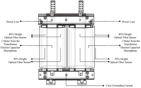
Figure 6.
On-site collected signal data and types.
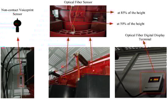
Figure 7.
On-site installation diagram of voiceprint sensor and fiber optic sensor.
4.2. Model Evaluation Metrics
The evaluation is performed using accuracy (ACC), recall (REC), specificity (SPE), and F1 score. The formulas for each evaluation metric are provided as follows:
In the formulas, TP represents the number of samples where both the model prediction and the true value are 1; TN denotes the number of samples where both the model prediction and the true value are 0; FP refers to the number of samples where the model predicts 1 but the true value is 0; FN corresponds to the number of samples where the model predicts 0 but the true value is 1; Precision (PRE) represents the proportion of actual positive samples among the samples predicted as positive.
4.3. HPO-DBN Feature Extraction Model Optimization Parameters
The DBN model is trained using an experimental setup based on the Windows 10 operating system, employing the CPU version of the TensorFlow framework. The programming environment is Python 3.7, with PyCharm 2023 utilized as the development tool. Model training is performed on an NVIDIA GeForce RTX 4070 GPU platform. The experiment is configured with 200 iterations, an RBM learning rate of 0.05, a fully connected layer learning rate of 0.1, a learning rate momentum of 0.02, and 800 neurons in the RBM layer. The dataset is partitioned into training and testing sets with a 6:4 ratio. Following the parameter input, feature vectors are extracted, and the resulting feature vectors are subsequently classified using an SVM classifier. The model evaluation parameters are detailed in Table 4.
Table 4.
DBN model parameter evaluation metrics.
As shown in Table 4, the ACC of the DBN-SVM model is 88.4%, REC is 87.1%, SPE is 86.7%, and the F1 score is 88.5%, indicating that the overall prediction performance is quite satisfactory. However, the number of RBM layers, the number of neurons in each RBM layer, and the learning rate are manually set, which introduces a certain degree of subjectivity. To improve the objectivity of parameter selection and further enhance model performance, this paper introduces the HPO algorithm to optimize the DBN model parameters. The HPO parameter settings are as follows: initial population size of 20; the termination condition is set to 200 iterations. The range for the number of hidden layers is [1, 5], the number of neurons per layer is [50, 1500], and the learning rate is [0.001, 0.1]. After initializing the model with the non-optimized DBN parameters and inputting the data, the optimizer determines the optimal number of layers, neurons, and learning rate after 200 iterations, as shown in Table 5. The SVM classifier is also used to classify the feature vectors, and the corresponding model evaluation parameters are presented in Table 6 below.
Table 5.
Optimal DBN parameters after iteration.
Table 6.
HPO-DBN model parameter evaluation metrics.
From the comparison between Table 5 and Table 6, it can be observed that the HPO-optimized DBN model outperforms the non-optimized DBN model in terms of accuracy. The ACC of the HPO-optimized model reaches 94.5%, with REC, SPE, and F1 score at 92.2%, 92.0%, and 93.4%, respectively—each of which surpasses the performance of the non-optimized DBN model. As shown in the figure, the loss curves for both the DBN and HPO-DBN models are provided. From Figure 8, it can be seen that the DBN model stabilizes around the 20th iteration, with the loss value eventually stabilizing around 1.2. In contrast, the HPO-optimized DBN model stabilizes around the 10th iteration, with the loss value reaching approximately 0.8, indicating a faster decline and lower loss value compared to the non-optimized DBN model.
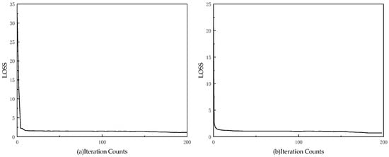
Figure 8.
Model loss curve graph. (a) Loss curve of the DBN model with the iteration counts; (b) Loss curve of the HPO-DBN model with the iteration counts.
4.4. Analysis of Voiceprint Feature Extraction Results
To evaluate the performance of the HPO-DBN feature extraction method, it is compared with the model proposed in Refs. [31,32,33,34]. For all methods, the feature vectors obtained after feature extraction are input into an SVM classifier for fault diagnosis. The bar chart illustrating the evaluation metrics for eight different methods in excitation transformer fault diagnosis is presented in Figure 9.
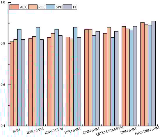
Figure 9.
Comparison of evaluation metrics for sight different models.
As shown in Figure 9, the HPO-DBN method outperforms the other models proposed in references [31,32,33,34] across all four evaluation metrics. Specifically, this method not only achieves higher accuracy (ACC) but also maintains a good balance with recall (REC), effectively reducing the occurrence of false positives and false negatives. Compared to the traditional SVM, HPO-DBN-SVM shows significant improvements in both accuracy and recall, indicating its ability to identify faulty samples more effectively and reduce missed detections. While IDBO-SVM and IGWO-SVM have made strides in parameter optimization, their performance still falls short of HPO-DBN-SVM, particularly in balancing recall and specificity. The HPO-DBN-SVM method excels in this balance. In terms of SPE, HPO-DBN-SVM accurately identifies negative class samples and reduces misdiagnosis. On the other hand, deep learning methods such as CNN-SVM and QPSO-LSTM-SVM show weaker performance in SPE. This is likely due to the complex feature extraction process, which may lead to misclassification of negative class samples, thereby reducing specificity.
This suggests that the HPO-DBN method not only has strong capabilities in identifying positive class samples but also effectively reduces false positives, ensuring the stability and reliability of the fault diagnosis system. Moreover, the improvement in the F1 score further confirms that the HPO-DBN method strikes a better balance between accuracy and recall, ensuring model stability across different samples. Compared to other methods, HPO-DBN-SVM enhances classification accuracy in complex fault conditions by optimizing feature extraction and model parameters, while effectively capturing voiceprint feature information. This provides robust support for the accurate identification of excitation transformer fault states.
4.5. Analysis of Temperature–Electrical Signal Feature Extraction Results
A total of 30 groups of signals were collected from the high- and low-voltage windings (three phases) of the excitation transformer, including winding temperature, power loss, and core grounding current. For each type of signal, 20-dimensional time-domain statistical features were extracted, resulting in a 600-dimensional time-domain feature set. The importance of these statistical features was evaluated using the Random Forest algorithm, with the number of decision trees set to 300. By comparing the classification performance under different feature dimensions, a curve illustrating the relationship between classification error and feature dimension was obtained, as shown in Figure 10.
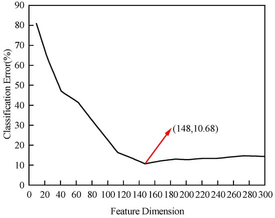
Figure 10.
Feature dimension analysis results.
According to the analysis results, the classification error is lowest at 10.86% when the top 148 feature dimensions are selected. To further reduce feature dimensionality and eliminate the impact of redundant features, this study employs an autoencoder network to fuse and reduce the dimensionality of the selected statistical features. By optimizing the number of neurons in the hidden layer of the autoencoder, the final value is set to 42, with the mean squared error (MSE) used as the loss function. The final model parameter settings are presented in Table 7.
Table 7.
Autoencoder parameters.
The feature vectors obtained after extraction are input into an SVM classifier for fault diagnosis. The confusion matrices for three conditions—normal state (I), DC bias magnetization state (II), and multi-point grounding state of the core (III)—are compared across three scenarios: using the original time-domain statistical features, the features filtered by Random Forest, and the features fused and reduced by the autoencoder. The results are presented in Figure 11.
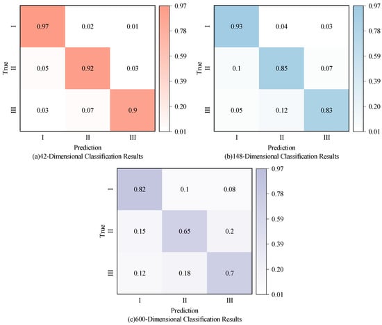
Figure 11.
Confusion matrices of classification results.
The results show that the classification accuracies on the test set for 42-dimensional, 148-dimensional, and 600-dimensional features are 93%, 87%, and 72%, respectively. When using the original 600-dimensional time-domain statistical features, the excessive number of irrelevant features overwhelms key information, negatively impacting classification performance. After feature selection using Random Forest, most irrelevant features are eliminated, resulting in an improvement of approximately 15% in model accuracy compared to the original feature set. However, some highly correlated redundant features remain. To address this, further nonlinear dimensionality reduction is performed using an autoencoder, which effectively removes redundant information, raising the final model accuracy to 93%. These results indicate that appropriate dimensionality reduction and feature selection can significantly enhance classification performance. Moreover, the combination of Random Forest and the autoencoder effectively reduces redundancy, improves computational efficiency, and boosts the model’s generalization ability.
4.6. Analysis of Fault Diagnosis Results
Based on the preprocessed feature vector data, this study conducts training and validation analysis of the proposed model. Several models—SVM, Adaboost-BP, XGBoost-SVM, and CNN—are selected for comparison with Adaboost-SVM, using the same input dataset. By comparing the evaluation metrics of each model, the effectiveness of the proposed fault diagnosis framework is validated. To minimize the influence of randomness, all models are tested 25 times, with the final overall classification performance reported as the average of these trials. The comparison results are summarized in Table 8, with evaluation metrics including average accuracy (PACC), average F1 score (PF1), average training time (Ttrain), and average testing time (Ttest).
Table 8.
Comparison of classification performance of different models.
From the comprehensive comparison of various metrics, it is evident that the Adaptive Boosting with Support Vector Machine (Adaboost-SVM) model performs the best in terms of average accuracy and average F1 score, achieving 96.89% and 96.48%, respectively. While ensuring high diagnostic accuracy, its training time is 1692.49 s, and its testing time is only 0.093 s, effectively balancing model accuracy and real-time performance. The Extreme Gradient Boosting with Support Vector Machine (XGBoost-SVM) model ranks second in classification accuracy, with PACC and PF1 values of 92.25% and 90.22%, respectively. It also exhibits relatively shorter training and testing times, demonstrating good efficiency and fast response capability. In contrast, although the Convolutional Neural Network (CNN) model maintains moderate performance with PACC (88.21%) and PF1 (85.30%), its training time is 5007.96 s, and testing time is 0.376 s, resulting in high training overhead and inference latency, making it unsuitable for real-time online diagnostic requirements. The Adaptive Boosting with Backpropagation (Adaboost-BP) model’s PACC (95.46%) and PF1 (92.74%) are close to those of XGBoost-SVM, but its training time (3030.62 s) and testing time (0.185 s) make it less efficient and real-time compared to the top two models. The traditional SVM model performs significantly worse in terms of PACC (74.90%) and PF1 (73.97%). While it has the shortest training time and the fastest inference speed, its classification accuracy is insufficient to meet the demands for high-reliability diagnostics. It should be noted, however, that baseline models such as SVM, CNN, and XGBoost-SVM were not optimized to the same extent as the proposed method. Future work will involve comprehensive hyperparameter tuning and the inclusion of state-of-the-art deep architecture to ensure fairer benchmarking and stronger comparative validation. Overall, Adaboost-SVM achieves a well-balanced trade-off between diagnostic accuracy, training cost, and inference efficiency, making it the most suitable model for online fault diagnosis of excitation transformers under complex operating conditions.
The classification performance of various models for normal operating conditions and faults, such as partial discharge, DC bias magnetization, component loosening, and multi-point grounding of the core, is shown in Figure 12.
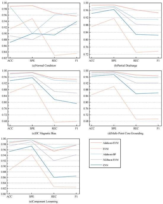
Figure 12.
Comparison of performance of five models under different operating conditions.
As shown in Figure 12, the Adaboost-SVM model exhibits strong generalization performance, achieving optimal values for ACC, REC, SPE, and F1 score in the recognition of partial discharge, DC bias magnetization, component loosening, and multi-point grounding of the core. Specifically, for the normal state, its F1 score is slightly lower than that of the Adaboost-BP model. In the recognition of component loosening faults, ACC and REC are slightly lower than those of the Adaboost-BP model. However, overall, Adaboost-SVM demonstrates the best performance across all evaluation metrics.
In summary, the Adaboost-SVM model excels in fault diagnosis accuracy, generalization ability, and real-time performance. It is well-suited to meet the practical demands for rapid response and precise classification in on-site operations.
5. Conclusions
This paper proposes a fault diagnosis method for excitation transformers based on HPO-DBN and multi-source heterogeneous information fusion. By integrating voiceprint signals, temperature, and electrical parameter data, the method significantly improves the accuracy and real-time performance of excitation transformer fault diagnosis. Specifically, HPO optimizes the DBN parameters, enabling the extraction of deep features closely related to faults from the voiceprint signals and effectively capturing the complex patterns of subtle faults. Building upon this, multi-source heterogeneous information is introduced, and features are dimensionally reduced using Random Forest and Autoencoder, which significantly reduces redundant information and enhances the diagnostic efficiency and accuracy of the model. Adaboost-SVM is employed as the classification model, and a working condition awareness mechanism is introduced, further enhancing the model’s generalization ability and real-time responsiveness, thus meeting the practical engineering application requirements for rapid diagnosis. The effectiveness of the proposed method is thoroughly validated through comparison experiments with other network models and multiple evaluation metrics. The main conclusions of this study are as follows:
- Compared to traditional methods such as SVM, Long Short-Term Memory (LSTM), and CNN, the HPO-DBN-based voiceprint signal feature extraction method significantly improves classification accuracy. The DBN optimized by HPO is more effective at extracting key information from high-noise voiceprint signals and capturing subtle fault features, thereby further enhancing the accuracy of fault diagnosis.
- The proposed temperature and electrical signal feature aggregation method effectively reduced the 600-dimensional time-domain statistical features to 42 dimensions, resulting in a 21% increase in diagnostic accuracy. By combining Random Forest for feature importance ranking with Autoencoder-based dimensionality reduction, redundant features were successfully eliminated, further improving the model’s computational efficiency and classification accuracy.
- Compared to traditional models such as SVM, XGBoost-SVM, and CNN, the proposed Adaboost-SVM model performs exceptionally well across multiple metrics, including accuracy, recall, and F1 score, achieving an overall accuracy of 96.89%. It demonstrates significant advantages in terms of real-time performance and diagnostic stability. By introducing a working condition awareness mechanism, Adaboost-SVM shows enhanced adaptability and robustness when facing complex operating conditions and multiple fault types, effectively addressing the fault diagnosis needs of excitation transformers in dynamic operating environments.
- The proposed fault classification method for excitation transformers demonstrates strong adaptability and stability under complex operating conditions. This method can also serve as a reference for the fault diagnosis of other power equipment, including transformers, motors, generators, circuit breakers, switchgear, as well as power capacitors and reactors. This highlights its broad potential for promotion and wide application prospects.
Author Contributions
Conceptualization, M.Y. and J.W.; methodology, Y.L. and P.B.; software, P.B.; validation, W.Z., Y.D., S.C. and P.B.; formal analysis, L.M.; investigation, P.Z.; resources, J.W.; data curation, J.D.; writing—original draft preparation, J.D.; writing—review and editing, P.Z.; visualization, M.Y.; supervision, J.W.; project administration, Y.L.; funding acquisition, M.Y. All authors have read and agreed to the published version of the manuscript.
Funding
This research was funded by China Yangtze Power Co., Ltd., grant number Z532402020.
Data Availability Statement
The data used in the analysis presented in the paper will be made available, subject to the approval of the data owner.
Conflicts of Interest
Authors Mingtao Yu, Yang Liu, Peng Bao, Weiguo Zu, Yinglong Deng, Shiyi Chen and Lijiang Ma were employed by the company China Yangtze Power Co., Ltd. The authors declare that this study received funding from China Yangtze Power Co., Ltd. The funder was not involved in the study design, collection, analysis, interpretation of data, the writing of this article or the decision to submit it for publication. The remaining authors declare that the research was conducted in the absence of any commercial or financial relationships that could be construed as a potential conflict of interest.
References
- Fu, X.; Guo, D.; Hou, K.; Zhu, H.; Chen, W.; Xu, D. Fault Diagnosis of an Excitation System Using a Fuzzy Neural Network Optimized by a Novel Adaptive Grey Wolf Optimizer. Processes 2024, 12, 2032. [Google Scholar] [CrossRef]
- Hussain, M.R.; Refaat, S.S.; Abu-Rub, H. Overview and partial discharge analysis of power transformers: A literature review. IEEE Access 2021, 9, 64587–64605. [Google Scholar] [CrossRef]
- Sun, L.; Xu, M.; Ren, H.; Hu, S.; Feng, G. Multi-point grounding fault diagnosis and temperature field coupling analysis of oil-immersed transformer core based on finite element simulation. Case Stud. Therm. Eng. 2024, 55, 104108. [Google Scholar] [CrossRef]
- Du, P.; Wang, B.; Xu, D. A minimum-order BEMF observer for DC-bias elimination of position-sensorless PMSM drives using backstepping design. IEEE Trans. Ind. Electron. 2024, 71, 13635–13649. [Google Scholar] [CrossRef]
- Zhang, Y.; Tang, Y.; Liu, Y.; Liang, Z. Fault diagnosis of transformer using artificial intelligence: A review. Front. Energy Res. 2022, 10, 1006474. [Google Scholar] [CrossRef]
- Cao, C.; Xu, B.; Li, X. Monitoring method on loosened state and deformational fault of transformer winding based on vibration and reactance information. IEEE Access 2020, 8, 215479–215492. [Google Scholar] [CrossRef]
- Zhao, P.; Wang, J.; Xia, H.; He, W. A novel industrial magnetically enhanced hydrogen production electrolyzer and effect of magnetic field configuration. Appl. Energy 2024, 367, 123402. [Google Scholar] [CrossRef]
- Zollanvari, A.; Kunanbayev, K.; Bitaghsir, S.A.; Bagheri, M. Transformer fault prognosis using deep recurrent neural network over vibration signals. IEEE Trans. Instrum. Meas. 2020, 70, 1–11. [Google Scholar] [CrossRef]
- Jia, S.; Jia, Y.; Bu, Z.; Li, S.; Lv, L.; Ji, S. Detection technology of partial discharge in transformer based on optical signal. Energy Rep. 2023, 9, 98–106. [Google Scholar] [CrossRef]
- Xian, R.; Wang, L.; Zhang, B.; Li, J.; Xian, R.; Li, J. Identification method of interturn short circuit fault for distribution transformer based on power loss variation. IEEE Trans. Ind. Inform. 2023, 20, 2444–2454. [Google Scholar] [CrossRef]
- Shih, K.J.; Hsieh, M.F.; Chen, B.J.; Huang, S.F. Machine learning for inter-turn short-circuit fault diagnosis in permanent magnet synchronous motors. IEEE Trans. Magn. 2022, 58, 8204307. [Google Scholar] [CrossRef]
- Ali, M.S.; Omar, A.; Jaafar, A.S.A.; Mohamed, S.H. Conventional methods of dissolved gas analysis using oil-immersed power transformer for fault diagnosis: A review. Electr. Power Syst. Res. 2023, 216, 109064. [Google Scholar] [CrossRef]
- Zhou, X.; Tian, T.; Li, X.; Chen, K.; Luo, Y.; He, N.; Zhang, G. Study on insulation defect discharge features of dry-type reactor based on audible acoustic. AIP Adv. 2022, 12, 025210. [Google Scholar] [CrossRef]
- Liu, H.; Gao, S.; Sun, L.; Tian, Y. Transformer winding deformation accompanied by magnetic flux leakage field distribution variation and its diagnostic analysis of deformation degree. J. Comput. Methods Sci. Eng. 2023, 23, 1517–1528. [Google Scholar] [CrossRef]
- Zhang, Y.; Li, J.; Liu, H.; Liu, R.; Yang, F.; Li, T. BP-Neural-Network-Based Aging Degree Estimation of Power Transformer Using Acoustic Signal. In Proceedings of the 2020 International Conference on Sensing, Measurement & Data Analytics in the Era of Artificial Intelligence (ICSMD), Xi’an, China, 15–17 October 2020; pp. 617–621. [Google Scholar]
- Li, H.; Yao, Q.; Li, X. Voiceprint fault diagnosis of converter transformer under load influence based on Multi-Strategy improved Mel-Frequency spectrum coefficient and Temporal convolutional network. Sensors 2024, 24, 757. [Google Scholar] [CrossRef]
- Yu, Z.; Wei, Y.; Niu, B.; Zhang, X. Automatic condition monitoring and fault diagnosis system for power transformers based on voiceprint recognition. IEEE Trans. Instrum. Meas. 2024, 73, 9600411. [Google Scholar] [CrossRef]
- Gong, C.; Peng, R. A novel hierarchical vision transformer and wavelet time–frequency based on multi-source information fusion for intelligent fault diagnosis. Sensors 2024, 24, 1799. [Google Scholar] [CrossRef]
- Cui, J.; Kuang, W.; Geng, K.; Jiao, P. Intelligent fault diagnosis and operation condition monitoring of transformer based on multi-source data fusion and mining. Sci. Rep. 2025, 15, 7606. [Google Scholar] [CrossRef]
- Hou, Y.; Wang, J.; Chen, Z.; Ma, J.; Li, T. Diagnosisformer: An efficient rolling bearing fault diagnosis method based on improved Transformer. Eng. Appl. Artif. Intell. 2023, 124, 106507. [Google Scholar] [CrossRef]
- Zhu, H.; He, Z.; Wei, J.; Wang, J.; Zhou, H. Bearing fault feature extraction and fault diagnosis method based on feature fusion. Sensors 2021, 21, 2524. [Google Scholar] [CrossRef]
- Xue, Y.; Wen, C.; Wang, Z.; Liu, W.; Chen, G. A novel framework for motor bearing fault diagnosis based on multi-transformation domain and multi-source data. Knowl.-Based Syst. 2024, 283, 111205. [Google Scholar] [CrossRef]
- Wang, Y.; Liu, Y.; Zhong, Z.; Jin, X.; Peng, Y.; Luo, J.; Yang, J. Gate-controlled silicon controlled rectifier with adjustable clamping voltage using a photoelectric mechanism. Opt. Express 2022, 31, 651–658. [Google Scholar] [CrossRef]
- Zhao, P.; Wang, J.; Sun, L.; Li, Y.; Xia, H.; He, W. Optimal electrode configuration and system design of compactly-assembled industrial alkaline water electrolyzer. Energy Convers. Manag. 2024, 299, 117875. [Google Scholar] [CrossRef]
- Marukatat, S. Tutorial on PCA and approximate PCA and approximate kernel PCA. Artif. Intell. Rev. 2023, 56, 5445–5477. [Google Scholar] [CrossRef]
- Guo, D.; Song, Z.; Liu, N.; Xu, T.; Wang, X.; Zhang, Y.; Cheng, Y. Performance study of hard rock cantilever roadheader based on PCA and DBN. Rock Mech. Rock Eng. 2024, 57, 2605–2623. [Google Scholar] [CrossRef]
- Naruei, I.; Keynia, F.; Sabbagh Molahosseini, A. Hunter–prey optimization: Algorithm and applications. Soft Comput. 2022, 26, 1279–1314. [Google Scholar] [CrossRef]
- Liu, G.; Li, L.; Zhang, L.; Li, Q.; Law, S.S. Sensor faults classification for SHM systems using deep learning-based method with Tsfresh features. Smart Mater. Struct. 2020, 29, 075005. [Google Scholar] [CrossRef]
- Kadhim, M.N.; Al-Shammary, D.; Mahdi, A.M.; Ibaida, A. Feature selection based on Mahalanobis distance for early Parkinson disease classification. Comput. Methods Programs Biomed. Update 2025, 7, 100177. [Google Scholar] [CrossRef]
- Tao, W.; Sun, Z.; Yang, Z.; Liang, B.; Wang, G.; Xiao, S. Transformer fault diagnosis technology based on AdaBoost enhanced transferred convolutional neural network. Expert Syst. Appl. 2025, 264, 125972. [Google Scholar] [CrossRef]
- Zhang, S.; Zhou, H. Transformer fault diagnosis based on Multi-Strategy enhanced Dung beetle algorithm and optimized SVM. Energies 2024, 17, 6296. [Google Scholar] [CrossRef]
- Wang, J.; Zhao, Z.; Zhu, J.; Li, X.; Dong, F.; Wan, S. Improved support vector machine for voiceprint diagnosis of typical faults in power transformers. Machines 2023, 11, 539. [Google Scholar] [CrossRef]
- An, Q.; Yang, P.; An, G.; Han, X.; Yang, X.; Li, Y.; Liu, D.; He, P.; Wang, S.; Gao, W. Feature Extraction and Fault Identification of Partial Discharge in Multi-signal Transformer. Sci. Technol. Eng. 2024, 24, 14699–14708. [Google Scholar]
- Zhang, H.; Wang, Z.; Zhou, H.; Zeng, S.; Yin, M.; Xu, J.; Zou, J. Intelligent fault prediction method for traction transformers based on IGWO-SVM and QPSO-LSTM. Int. J. Power Energy Convers. 2024, 15, 408–424. [Google Scholar] [CrossRef]


Disclaimer/Publisher’s Note: The statements, opinions and data contained in all publications are solely those of the individual author(s) and contributor(s) and not of MDPI and/or the editor(s). MDPI and/or the editor(s) disclaim responsibility for any injury to people or property resulting from any ideas, methods, instructions or products referred to in the content. |
© 2025 by the authors. Licensee MDPI, Basel, Switzerland. This article is an open access article distributed under the terms and conditions of the Creative Commons Attribution (CC BY) license (https://creativecommons.org/licenses/by/4.0/).