Article

Multi-Resolution LSTNet Framework with Wavelet Decomposition and Residual Correction for Long-Term Hourly Load Forecasting on Distribution Feeders

1
Smart Power Distribution Laboratory, Korea Electric Power Corporation Research Institute, Daejeon 34056, Republic of Korea
2
School of Electronic and Electrical Engineering, Hankyong National University, Anseong 17579, Republic of Korea
*
Author to whom correspondence should be addressed.
Energies 2025, 18(20), 5385; https://doi.org/10.3390/en18205385
Submission received: 11 September 2025 / Revised: 4 October 2025 / Accepted: 9 October 2025 / Published: 13 October 2025
(This article belongs to the Special Issue New Progress in Electricity Demand Forecasting)

Abstract

Distribution-level long-term load forecasting with hourly resolution is essential for modern power systems operation, yet it remains challenging due to complex temporal patterns and error accumulation over extended horizons. This study proposes a Multi-Resolution Residual LSTNet framework integrating Discrete Wavelet Transform (DWT), Long Short-Term Memory Networks (LSTNet), and Normalized Linear (NLinear) models for accurate one-year ahead hourly load forecasting. The methodology decomposes load time series into daily, weekly, and monthly components using multi-resolution DWT, applies direct forecasting with LSTNet to capture short-term and long-term dependencies, performs residual correction using NLinear models, and integrates predictions through dynamic weighting mechanisms. Validation using five years of Korean distribution feeder data (2015–2019) demonstrates significant performance improvements over benchmark methods including Autoformer, LSTM, and NLinear, achieving Mean Absolute Error of 0.5771, Mean Absolute Percentage Error of 17.29%, and Huber Loss of 0.2567. The approach effectively mitigates error accumulation common in long-term forecasting while maintaining hourly resolution, providing practical value for demand response, distributed resource control, and infrastructure planning without requiring external variables.

1. Introduction

Long-Term Load Forecasting (LTLF) is widely recognized as an essential tool for ensuring the stable operation of power systems and supporting long-term resource planning. As noted by Lindberg et al. [1], LTLF provides the foundation for determining future electricity demand, transmission and generation capacity, and plays a critical role in strategies for infrastructure expansion, asset replacement, and generation mix transitions. Similarly, Carvallo et al. [2] emphasized that LTLF serves as a central input for Integrated Resource Planning (IRP), enabling coherent decision-making among policymakers, utilities, and regulatory authorities.
Driven by these needs, recent studies have sought to enhance the accuracy of LTLF through advanced modeling techniques. Zhang et al. [3] transformed yearly and monthly load profiles of distribution transformers into image representations and applied Convolutional Neural Networks (CNN) for image representation learning, achieving mean absolute percentage errors (MAPE) around 13%, with some cases as low as 9–10%. Mathew et al. [4] combined XGBoost with a Prominence-guided Weighted Peaks (PWP) method for feeder-level medium-term forecasting, incorporating daily to monthly series and exogenous variables to improve peak load predictions. Matrenin et al. [5] employed ensemble machine learning (Random Forest, XGBoost, AdaBoost) in isolated systems, finding Random Forest to be the most reliable for multi-year forecasts. Butt et al. [6] applied CNNs, LSTMs, and MLPs—individually and in combination—for feeder-level horizons up to six years, reporting MAPE values of 2–3%. At the national scale, Lee [7] combined regression-based models with exogenous factors such as temperature and industrial indices to forecast South Korea’s total consumption, yielding MAPE near 2%. Similarly, Jung et al. [8] applied transfer learning with deep neural networks (DNNs) for district-level demand in Seoul, achieving MAPE of 6.6%.
Several other works extend LTLF to system-wide or national contexts. Wen et al. [9] developed a hybrid of Takagi–Sugeno fuzzy models and RBF-based recurrent neural networks, reducing RMSE and MAPE by 2–3 percentage points compared to GA-LSTM. Liu et al. [10] decomposed national monthly demand with Ensemble Empirical Mode Decomposition (EEMD) and forecasted each component with Random Forests, reaching an MAPE of 2.14%. Wang et al. [11] proposed an Informer–LSTM ensemble for multi-week to multi-month horizons, achieving low MSE and MAE. Farrag et al. [12] applied GA-optimized Stacked LSTM for 10-year-ahead forecasting in South Australia, achieving sub-1% MAPE. Rubasinghe et al. [13] used a CNN–LSTM sequence-to-sequence model for 3-year monthly peak forecasting, reporting MAE of 499.85 MW and MAPE of 4.29%. Peng et al. [14] introduced a decomposition approach separating industrial and temperature-sensitive components, reducing MAPE to 1.5–3%. Fan et al. [15] proposed a hybrid Crisscross Feature Collaboration (CFC) with Hierarchical Highway Networks (HHN), significantly improving RMSE by 84–94%. Dong et al. [16] developed a selective sequence-learning multi-layer RNN for Canadian feeder data, outperforming bottom-up/top-down strategies. Similarly, Tai et al. [17] proposed an ANN-based long-term forecasting model for Malaysia, incorporating input and model uncertainties to achieve R2 = 0.9994, outperforming SARIMA baselines.
Although most studies rely on monthly or daily aggregation, a limited number have addressed high-resolution, time-domain long-term forecasts. Ozdemir [18] employed a probabilistic cumulative distribution function model for one-year horizons at hourly/daily resolution, with scenario-based MAPE between 2.56–4.64%. Nabavi et al. [19] combined Discrete Wavelet Transform (DWT) with LSTM for horizons up to one year, across Iranian and German datasets, achieving MAPE as low as 0.29%. In a related study, Grandón et al. [20] proposed a hybrid approach combining classical statistical models with LSTM-based residual prediction for Ukraine’s hourly demand forecasting, achieving 96.83% accuracy.
Nevertheless, a common limitation of prior work is that distribution-line-level LTLF with hourly resolution maintained over horizons of one year or more remains largely unexplored. Existing efforts at this granularity have primarily focused on national, urban, or household-level demand. Yet, such fine-grained forecasts are critical in distribution systems where sharp hourly fluctuations can directly trigger voltage instability, power factor deterioration, and equipment overloading—ultimately affecting the operational efficiency of distributed energy resources such as demand response (DR), energy storage systems (ESS), and photovoltaic (PV) inverters [14]. With the growing penetration of Advanced Metering Infrastructure (AMI) and widespread access to high-resolution smart meter data, conventional models based on low-resolution aggregated series are increasingly inadequate [21,22].
The present study addresses this gap by developing a forecasting framework for distribution feeders that maintains hourly resolution while extending prediction horizons to one year or longer. This approach seeks to provide both practical utility for system operation and resource planning, and technical relevance in managing distributed resources under modern grid conditions. The paper is organized as follows: Section 2 introduces the distribution feeder dataset and its characteristics. Section 3 details the proposed framework combining Discrete Wavelet Transform (DWT) with an LSTNet-based predictive model. Section 4 evaluates performance against multiple baselines through extensive experiments. Finally, Section 5 summarizes the findings, outlines implications for grid operation and planning, and discusses future directions.

2. Data Acquisition and Description

The load data used in this study were collected from the Substation Operation Management System (SOMAS) operated by Korea Electric Power Corporation (KEPCO). SOMAS continuously monitors and records the operating status of substation equipment. In particular, the system measures the total active power of each distribution feeder at the outgoing circuit breaker (CB) with a sampling interval of 30 s, and aggregates these measurements into hourly records for storage and management.
For the present work, we utilized hourly load time series data collected from the Gangoe distribution feeder connected to the Seocheongju substation in Chungcheongbuk-do, South Korea. The dataset spans a five-year period from January 2015 to December 2019. Among them, the data from 2015 to 2018 were used for model training, while the data from 2019 were reserved exclusively for evaluation and testing. The Gangoe feeder serves a mixed commercial–residential area, exhibiting diverse temporal characteristics such as intra-day variability, seasonality, weekday–weekend differences, and occasional anomalous patterns. The time series profile and statistical distribution of the data are presented in Figure 1.
In many previous LTLF studies, exogenous variables such as temperature, humidity, and calendar information have been included to improve predictive accuracy. While this approach may yield benefits for national- or regional-level demand forecasts, or for specific end-use cases such as individual buildings, it may introduce complexity and practical limitations at the distribution-feeder level. Integrating external weather data requires careful evaluation of variable contributions and consistency, and may increase model complexity to the point of reducing operational feasibility in real-world deployment. For this reason, we adopted a simplified modeling approach by using only feeder-level load values as inputs. This design enhances data reliability and resolution while ensuring practical ease of data acquisition and streamlined operation in actual power systems.
To analyze temporal characteristics and extract long-term trends, we applied the Discrete Wavelet Transform (DWT) to the feeder load series. DWT is particularly effective at attenuating high-frequency noise, allowing us to limit preprocessing to basic gap-filling through interpolation [23]. Beyond preprocessing, DWT also serves as a core analytical tool within the proposed forecasting framework, and its structural details and implementation are further elaborated in Section 3.

3. Multi-Resolution Wavelet–Neural Forecasting Framework

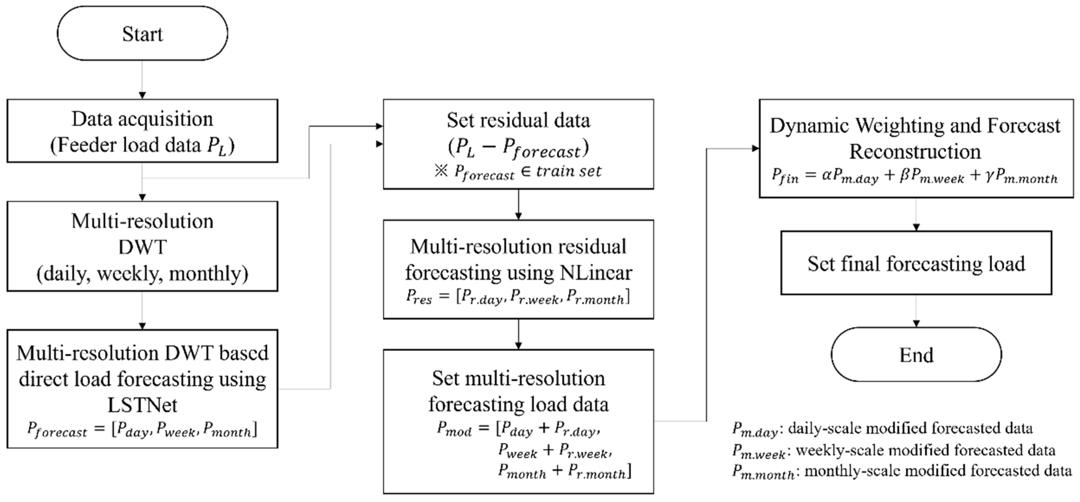
In this study, we propose a long-term load forecasting framework that combines multi-resolution Discrete Wavelet Transform (DWT), the Long- and Short-Term Time-series Network (LSTNet), and residual correction using the NLinear model. The proposed forecasting process consists of four sequential stages. In the first stage, the time series load data are decomposed into multiple scales using DWT. In the second stage, the decomposed series at each scale are independently forecasted using LSTNet to capture both short- and long-term dependencies. In the third stage, the discrepancies between the LSTNet predictions and the actual load values are treated as residual errors, which are subsequently learned and corrected by the NLinear module. In the final stage, the scale-wise forecasts are adaptively integrated into a single final forecast through a dynamic weighting mechanism. In this framework, only historical load data were used as input variables, without incorporating any exogenous features such as weather or calendar information. This design choice ensures a univariate forecasting structure that emphasizes the intrinsic temporal patterns of the load series. A schematic diagram of the proposed forecasting procedure is presented in Figure 2. The following subsections describe in detail the theoretical background, design rationale, and mathematical formulations underlying each step of the framework.

3.1. Multi-Resolution Discrete Wavelet Transform for Load Decomposition

The Discrete Wavelet Transform (DWT) is a representative technique for decomposing time-series signals into a multi-resolution form, offering the advantage of simultaneously capturing information in both the time and frequency domains [24]. A time-series signal x ( t ) can be expressed by DWT as shown in Equations (1) and (2):
x t = x ¯ j t + j = 1 J d j ( t )
d j t = k = 0 K j 1 d j , k · ψ j , k t
where x ¯ j t denotes the low-frequency approximation component at level j , d j ( t ) represents the high-frequency detail component at level J , ψ ( t ) is wavelet basis function, j refers to the time scale, k indicates the shift along the time axis, and K j is the number of possible shifts defined at scale j .
Furthermore, in Equations (1) and (2), each d j ( t ) reflects the variability at a specific time scale and is defined through the wavelet basis function ψ ( t ) as shown in Equation (3):
ψ j , k t = 2 j / 2 ψ 2 j t k
In other words, ψ ( t ) determines the fundamental form of the entire family of wavelet functions, where j represents the scale and k denotes the shift. This formulation implies two important properties. First, the scaling factor 2 j controls the dilation of the wavelet function along the time axis; as the scale increases, the time resolution decreases and the function captures lower-frequency components. Second, the shift parameter k determines the position of the wavelet function within the time series. Consequently, each wavelet function ψ j , k ( t ) is able to capture signal components with periodicities of approximately 2 j time units. For example, when j = 5 , variations with a period of roughly 32 h can be represented, while j = 8 corresponds to a period of about 256 h (approximately 11 days). Based on this relationship between wavelet scales and temporal periodicities, this study sets the DWT levels to correspond to three major cycles commonly observed in power load time series—daily (24 h), weekly (168 h), and monthly (720 h). For each scale, the DWT is applied independently, and only the approximation coefficients corresponding to that scale are retained to reconstruct the low-frequency component. As a result, multi-resolution time series representations at daily, weekly, and monthly levels are obtained, as illustrated in Figure 3. In practice, however, we implement a wavelet-inspired causal multi-resolution filtering. This design is motivated by the DWT framework and realized in a causal manner, using only past observations at each prediction step. Without preserving the strict orthogonality of the standard DWT, this adaptation effectively prevents information leakage while maintaining the multi-resolution interpretability necessary for forecasting.
Unlike most existing DWT-based forecasting studies, which generally perform a single transformation to handle multiple frequency components collectively, this study applies DWT separately at explicit scale levels to enable scale-wise analysis grounded in physical periodicities. This approach not only enhances interpretability but also allows the distinctive load characteristics at each resolution to be more clearly represented, thereby providing an important differentiation from conventional methods. Furthermore, as noted earlier, the wavelet transformation inherently attenuates high-frequency noise, and therefore no additional preprocessing was required beyond simple linear interpolation for missing values [23].

3.2. Direct Load Forecasting Using Multi-Resolution LSTNet

The forecasting method proposed in this study adopts a direct forecasting strategy for time-series components decomposed by the multi-resolution Discrete Wavelet Transform (DWT). In general, multi-step ahead forecasting approaches can be categorized into two strategies. The first involves iteratively applying a one-step-ahead prediction model until the desired horizon is reached. The second directly predicts the target value at a specific future horizon without intermediate steps. While the iterative approach may be effective for short-term horizons, its accuracy deteriorates over longer horizons due to error accumulation across successive steps. By contrast, the direct forecasting approach models the target value explicitly at the forecasting horizon, thereby eliminating error propagation and improving long-term reliability [25]. Since the objective of this study is long-term load forecasting over a one-year horizon, the direct forecasting method was selected to effectively mitigate the degradation of accuracy caused by error accumulation. More specifically, the proposed framework forecasts monthly load values directly from historical load data and repeats this process twelve times to construct a one-year forecast sequence.
For the forecasting model, we employed the Long- and Short-Term Time-series Network (LSTNet), which is designed to effectively capture both short- and long-term dependencies in time-series data. LSTNet was originally developed to overcome the performance limitations of conventional Recurrent Neural Network (RNN)-based models in long-horizon forecasting by integrating Convolutional Neural Networks (CNN) and a skip-RNN structure. The CNN module efficiently extracts local features from the input time series, while the skip-RNN module addresses the difficulty of standard RNNs in learning long-term dependencies by explicitly encoding periodic patterns. Consequently, LSTNet has been reported to achieve superior forecasting performance, particularly for time-series data characterized by strong temporal correlations and distinct periodicities [26].

3.2.1. Direct Forecasting Method

In time-series forecasting, direct forecasting refers to the strategy of constructing an independent prediction model for each forecasting horizon, thereby estimating the target value at that horizon without passing through intermediate steps. This approach contrasts with iterated forecasting, in which a one-step-ahead model is repeatedly applied to generate long-term forecasts. The latter inherently suffers from error accumulation, since each forecasted value becomes the input for subsequent predictions, leading to compounding errors over longer horizons. By contrast, direct forecasting assigns an independent prediction pathway to each horizon, thereby preventing the propagation of errors and offering a distinct advantage for long-term forecasting.
Traditionally, direct forecasting has been formulated using autoregressive (AR) models. For a forecasting horizon h , an AR-based direct forecasting model is defined as (4)
y t + h h = β + i = 1 p ρ i y t + 1 i + ε t + h
where y t + h h denotes the forecast at horizon h from time t , β ,   ρ i are the model parameters, p is the autoregressive order, and ε t + h represents the error term.
In other words, this formulation differs from the iterated forecasting approach in that each forecasting horizon is associated with its own unique set of parameters. According to Marcellino et al. [25], even in the presence of model misspecification or structural breaks in the time series, the direct forecasting approach has been shown to outperform the iterative method.
In this study, we adopt the direct forecasting strategy to leverage these advantages for long-term load forecasting. Specifically, the forecasting model f θ h in the direct approach is replaced by the LSTNet-based architecture described in the following subsection. Accordingly, the direct forecasting framework can be generalized as shown in Equation (5):
y ¯ t + h h = f θ h x t p + 1 : t
where x t p + 1 : t denotes the input time-series data, and f θ h is the forecasting function that incorporates the learnable parameters θ .
Since the model is trained independently for each forecasting horizon, it effectively avoids the cascade errors inherent in iterative forecasting and enables model optimization tailored to the characteristics of each horizon. Building on this direct forecasting framework, the present study designs a model that predicts monthly load values and repeats this procedure twelve times to construct a full one-year load forecast sequence. This process can be formulated as shown in Equation (6):
Y 1 y e a r = y ¯ t + 1 : t + 730 h , y ¯ t + 731 : t + 1460 h , , y ¯ t + 8031 : t + 8760 h
Each forecast at a given horizon is independently generated by a model f θ h corresponding to a fixed monthly input window, providing a foundation for achieving both stability and scalability in long-term forecasting. In particular, in this study, each input window is composed of multi-resolution DWT-based components (daily, weekly, and monthly), which not only preserve long-term periodic information but also enhance the training efficiency of the forecasting model.

3.2.2. LSTNet-Based Load Forecasting Architecture

The Long- and Short-Term Time-series Network (LSTNet) is a deep learning-based model proposed by Lai et al. (2018) [26] for effectively forecasting time-series data characterized by complex periodicities and nonlinearities. Traditional forecasting models such as ARIMA or simple RNNs are effective in capturing short-term patterns or linear dependencies but exhibit structural limitations in reflecting long-term periodicity and complex multivariate interactions. To address these challenges, LSTNet integrates Convolutional Neural Networks (CNN), Recurrent Neural Networks (LSTM), a skip-recurrent structure, and a linear Autoregressive (AR) component into a unified framework, thereby enabling the simultaneous learning of diverse temporal patterns within the time series. LSTNet has demonstrated superior performance in forecasting problems involving fixed periodicities and is widely regarded as a powerful architecture with applicability across various domains [27].
LSTNet processes the input time series through a multi-layer neural network structure consisting of four primary components. First, the CNN module is employed to capture local patterns within short temporal segments of the input series. For an input sequence X = [ x t ω + 1 , , x t ] , the CNN performs one-dimensional convolutions along the time axis using k kernels with a kernel size of s . Each kernel extracts local features from the time series, and the CNN output is defined in Equation (7):
C t , j = R e L U i = 0 s 1 W j , i · x t i + b j  
where W j , i denotes the filter weight of the i -th element in the j -th kernel, b j is the bias term. The resulting feature vector C t = [ C t , 1 , , C t , k ] is then passed as input to the subsequent LSTM module.
Second, the RNN module receives the CNN output C t in temporal order to learn the sequential dependencies of the time series. In this study, the RNN module is implemented using the Long Short-Term Memory (LSTM) network, which has strong capabilities in handling long-term dependencies and capturing temporal patterns [28,29,30]. LSTM maintains long-range dependencies through its input, forget, and output gates, while the internal cell state enables stable learning of temporal dynamics. The computational process of LSTM is defined in Equations (8)–(12), and the output of the RNN module is denoted as h t L S T M . This output serves as the representation at time t within the LSTM block and is subsequently utilized in the skip-RNN and AR modules for generating the final forecast:
f t = σ W f C t + U f h t 1 + b f
i t = σ W i C t + U i h t 1 + b i
o t = σ W o C t + U o h t 1 + b o
c t = f t × c t 1 + i t × tanh W c C t + U c h t 1 + b c
h t L S T M = o t × tanh c t
where f t ,   i t ,   o t denote the forget, input, and output gates, respectively, C t is the feature vector at time t extracted from the CNN module, h t L S T M is the hidden state at time t , c t is the cell state, W ,   U ,   b represent the trainable weights and biases, and σ is the sigmoid activation function.
Third, the skip-RNN module is designed to explicitly capture long-term periodicity, which is particularly important in data such as electricity demand where recurring patterns occur at fixed times of the day. The skip-RNN module takes as input the sequence of hidden state vectors h t L S T M generated by the LSTM and models long-term periodic dependencies. As shown in Equation (13), the module incorporates the hidden state from a previous cycle ( t p ) to repeatedly reference past information at the same time of day, thereby reflecting the long-term periodic structure of the time series,
h t S k i p = 1 u t × h t p L S T M + u t × R e L U h t L S T M W x c + r t × h t p L S T M W h c + b c
where p denotes the periodic length, r t and u t are the reset and update gates, h t p L S T M is the hidden state from the previous cycle, W x c and W h c are the input-to-hidden and hidden-to-hidden weights, respectively, and b c is the bias term.
Fourth, the autoregressive (AR) module is incorporated to compensate for the limitation that deep neural networks are often insensitive to scale variations in the input time series. This component performs a linear prediction based on the most recent values of the input and acts as a linear correction term to the overall output. By integrating these four modules, the final forecast y ¯ t is defined as shown in Equation (14):
y ¯ t = h t L S T M + h t S k i p + h t A R
Each term in Equation (14) corresponds to the outputs of the LSTM, skip-RNN, and AR modules, respectively, capturing short-term patterns, long-term periodicity, and linear trend components. By summing these contributions, the model integrates multiple structures inherent in the time series into a unified representation. In this study, this baseline architecture is further enhanced with multi-resolution time-series analysis using DWT. Specifically, separate LSTNet models are applied to the daily, weekly, and monthly components obtained through DWT decomposition. The forecasts at each resolution are subsequently refined using an NLinear-based residual correction module, and the final prediction is derived by dynamically weighting the corrected results through a gating network.
Power demand time series are characterized by scale variations associated with daily, weekly, and seasonal periodicities. To effectively capture such complex patterns, an integrated forecasting framework that simultaneously accounts for short- and long-term dependencies, linear and nonlinear dynamics, and both local and global characteristics is required. LSTNet is designed to meet these requirements by combining CNN-based short-term feature extraction, LSTM-based temporal dynamics modeling, skip-RNN-based periodic encoding, and AR-based linear correction, while the integration of multi-resolution analysis further improves the precision and robustness of the forecasts.

3.3. Residual Learning Using NLinear

Recent studies on time-series forecasting have raised concerns that Transformer-based models may be less suitable for long-term series forecasting (LTSF) due to their structural complexity and limited sensitivity to temporal order. To address these limitations, Zeng et al. (2023) [31] proposed LTSF-Linear, a family of single-layer linear models. Among these, the Normalized Linear (NLinear) variant provides a simple yet effective mechanism for correcting distributional shifts in time-series data. In this study, NLinear is integrated into the proposed multi-resolution LSTNet architecture to perform residual correction on the forecasts.
NLinear is a single-layer linear regression model operating along the temporal dimension, directly transforming the input time series to generate forecasts for future time steps. The model can be summarized in two key steps: first, the input sequence X = [ x 1 , x 2 , , x L ] is normalized relative to its last value, and second, a linear transformation is applied to the normalized series, after which the last value is added back to restore the original scale. This process is expressed in Equation (15):
y ^ = W X x L + x L
where X is the input sequence of length L , x L denotes the last observation, W is the weight matrix for the linear transformation, and y ^ is the predicted output.
This structure also corresponds to direct multi-step forecasting, providing the advantage of effectively avoiding the error accumulation problem that frequently arises in long-term forecasting. In addition, it is sensitive to scale shifts and drift in the input series, which are corrected through normalization, and its simple structure allows for fast training and high interpretability [31].
In this study, independent NLinear blocks are constructed for the forecasts generated by the LSTNet-based architecture at different resolutions: daily, weekly, monthly. Each block learns the residuals between the predicted and actual load values and provides linear corrections, resulting in residual terms r d ,   r w ,   r m respectively. The corrected forecasts at each resolution can then be expressed as
y ̿ t = y ¯ t . d + r d ,   y ¯ t . w + r w ,   y ¯ t . m + r m
where each term represents the refined prediction for the corresponding resolution after residual adjustment.
By employing the NLinear-based residual forecasting approach, partial errors that may be overlooked by more complex models can be corrected through a simpler structure, thereby improving the overall accuracy and stability of the forecasts. In particular, this method linearly offsets potential biases or scale mismatches that may arise from the nonlinear estimation results of LSTNet, which enhances both the robustness and the generalization capability of the proposed model [32].

3.4. Dynamic Weighting and Forecast Integration

As described above, in the LSTNet-based multi-resolution forecasting architecture, forecasts and residual-corrected outputs are generated independently for the daily, weekly, and monthly time series. Therefore, a final integration step is required. Instead of a simple averaging approach, this study adopts a dynamic weighting strategy, which allows the relative importance of each resolution to be flexibly reflected depending on the forecasting context [33].
In the proposed framework, the importance of each resolution at a given time step is adaptively determined by a neural network. Specifically, the mean absolute values of the residual corrections are used as inputs to a softmax function, which produces the dynamic weights α d ,   α w ,   α m for the daily, weekly, and monthly resolutions, respectively, as shown in
α = S o f t m a x W g · r d , r w , r m + b g
where α = α d ,   α w ,   α m , r d ,   r w ,   r m denote the residual corrections from the NLinear modules, an W g ,   b g are the learnable parameters of the gating network. The final corrected forecast Y ¯ t is then obtained as
Y ¯ t = α d y ¯ t . d + r d + α w y ¯ t . w + r w + α m y ¯ t . m + r m
which represents the weighted combination of the residual-corrected forecasts at each resolution.
The rationale for adopting dynamic weighting is threefold. First, fixed-weight integration assigns the same importance across all time steps and therefore fails to capture the varying reliability of information inherent in real power demand data. In contrast, dynamic weighting can flexibly respond to time-dependent forecasting reliability, leading to more accurate predictions. Second, residual-based weighting leverages a direct measure of forecasting error, allowing adaptive integration that is based not only on intrinsic time-series patterns but also on the actual predictive performance. Third, the use of softmax normalization ensures a balanced contribution of each resolution to the overall forecast, while preventing over-reliance on any single resolution.
In conclusion, this study integrates the resolution-specific forecasts and residual corrections through a gating network with dynamic weighting, thereby achieving both stability and flexibility in predictive performance. This integration strategy effectively captures the irregularity of real-world power demand and quantitatively reflects the variation in forecast reliability across different time steps.

4. Verification of Proposed Method

In this section, the predictive performance of the proposed multi-resolution LSTNet–Residual model is evaluated using multiple analytical metrics and compared against representative baseline models that are widely employed in the field of long-term load forecasting. For experimental validation, the model was trained on load data from 2015 to 2018 and evaluated on the 2019 data, ensuring a strict separation between training and testing sets. Specifically, Mean Absolute Error (MAE) and the Huber loss are adopted as evaluation metrics, in order to simultaneously account for absolute forecasting accuracy and robustness to outliers.
The Mean Absolute Error (MAE) measures the average magnitude of the absolute differences between the predicted and actual values, and is defined as in Equation (19),
M A E = 1 N i = 1 N y i Y ¯ i
where y i and Y ¯ i represent the actual and predicted load of the feeder, respectively, and N denotes the number of samples. Because it reflects the average absolute error regardless of its direction, MAE provides an intuitive measure of predictive performance, particularly suitable for time-series forecasting problems such as power demand where the scale remains relatively stable.
The Huber loss is a loss function that combines the characteristics of Mean Squared Error (MSE) and Mean Absolute Error (MAE). It behaves like the squared error for small deviations and like the absolute error for large deviations, thereby reducing sensitivity to outliers. In this study, the threshold parameter δ was set to 1.0, which provides a good balance between sensitivity to small errors and robustness to outliers. Since the load values were normalized prior to training, this choice was found appropriate for stable optimization, and hyperparameter tuning was carried out in the direction of minimizing the Huber loss, thereby ensuring stable and robust training performance. The Huber loss is formulated as in Equation (20):
H u b e r y ,   Y ¯ = 1 2 y Y ¯ 2 w h e n   y Y ¯ δ δ y Y ¯ 1 2 δ w h e n   y Y ¯ > δ
In this study, the Huber loss is employed to mitigate the influence of outliers during training and evaluation, thereby ensuring more stable forecasting performance. Particularly for power demand time series that may contain occasional anomalies, the Huber loss serves as an effective evaluation metric for enhancing model robustness.
For comparison with the proposed model, we evaluated several representative models that are frequently used in long-term time series forecasting, including Autoformer, LSTM, and NLinear. Autoformer is a Transformer-based model that decomposes time-series inputs into trend and seasonal components through a decomposition-based attention mechanism, thereby improving forecasting efficiency and maintaining stable performance even over long horizons. LSTM, with its ability to handle long-term dependencies and capture temporal patterns, has been widely recognized as a strong baseline for time-series prediction. NLinear, while based on a simple linear structure, provides a meaningful benchmark because it stabilizes non-stationary distributions through normalization and supports direct multi-step forecasting [28,29,30,31,34].
The performance comparison with these baseline models confirms the effectiveness of the proposed approach in addressing the challenges of long-term load forecasting. A summary of the quantitative results is provided in Table 1, while Figure 4, Figure 5, Figure 6 and Figure 7 illustrate the predicted and actual values for each model. The analysis demonstrates that the proposed model consistently achieves the lowest MAE and Huber loss across all evaluation metrics, with the performance gap becoming more pronounced as the forecasting horizon increases. In conclusion, the proposed Multi-resolution Residual LSTNet effectively integrates information from multiple temporal resolutions, applies residual correction and dynamic weighting, and thereby secures higher accuracy and robustness compared to existing long-term forecasting models.
As shown in Table 1, the proposed Multi-resolution Residual LSTNet outperformed all baseline models across evaluation metrics, achieving an MAE of 0.5771, an MAPE of 17.29%, an RMSE of 0.7606, and a Huber loss of 0.2567. In particular, it recorded a substantially lower error compared to Autoformer (MAPE 33.67%) and LSTM (MAE 0.7258, RMSE 0.8994), and also outperformed the simple linear-based NLinear in terms of MAE and Huber loss. These differences are further illustrated in Figure 4, Figure 5, Figure 6 and Figure 7: while LSTM and Autoformer exhibited large deviations from the actual values during low-load periods in summer and peak-load periods in winter, the proposed model effectively captured both trend variations and short-term fluctuations, thereby maintaining close alignment with the observed data.
Although the performance improvements over the NLinear baseline appear numerically small, the proposed model consistently achieved lower MAE (0.5771 vs. 0.5837), RMSE (0.7606 vs. 0.7973), and Huber loss (0.2567 vs. 0.2702). This consistency across multiple metrics indicates that the proposed framework is not only marginally more accurate but also more stable and robust than NLinear. In long-term load forecasting, even a 1–2% reduction in error can have meaningful implications for operational cost and reliability management, underscoring the practical value of these improvements.
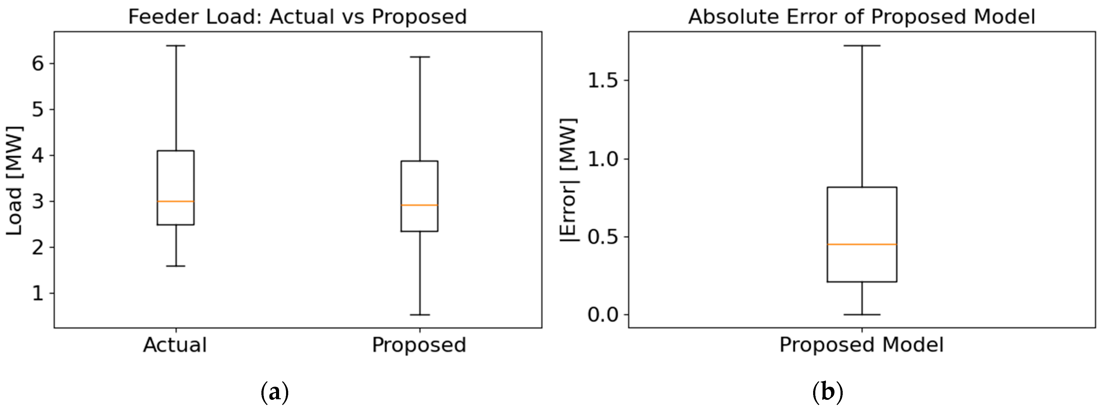
Figure 8 presents boxplots illustrating both the comparison between actual feeder load and the values predicted by the proposed model (a), and the distribution of absolute prediction errors (b). In panel (a), the actual and predicted load distributions exhibit similar medians and interquartile ranges, indicating that the proposed model closely reproduces the central tendency and variability of the observed load. Although some discrepancies appear at the lower extreme values, long-term load forecasting primarily relies on accurately estimating peak loads for capacity planning and reliability management. In this regard, the comparable upper extremes and overall spread suggest that the proposed model provides sufficiently robust performance for practical power system applications. Panel (b) further shows that the absolute errors are mostly concentrated below 1 MW, with a median of approximately 0.45 MW. This demonstrates that the proposed model achieves stable accuracy and maintains robustness across different load conditions.
Moreover, in long-term forecasting it is common for seasonal variations, irregularities in peak and trough loads, and external disturbances to accumulate and significantly amplify errors. Since comparable studies at the distribution feeder level with one-year ahead hourly resolution are very limited and industry guidelines do not provide explicit thresholds for acceptable MAPE values, direct benchmarking is difficult. Nevertheless, under such challenging conditions, the fact that the proposed model maintained an MAPE below 20% demonstrates its capability to stably reproduce long-term trends and seasonal variations while suppressing excessive deviations at extreme points. This indicates that the proposed approach not only achieves lower average error values but also provides a reliable foundation for capacity planning, peak load management, and demand-side decision making in practical power system operations.

5. Conclusions

This study proposed a novel framework for long-term load forecasting at the distribution feeder level while preserving high temporal resolution at the hourly scale. The proposed Multi-resolution Residual LSTNet combines multi-resolution DWT-based decomposition, LSTNet for capturing both short- and long-term patterns, NLinear-based residual correction, and dynamic weighting integration, thereby overcoming structural limitations of conventional long-term forecasting models. Experimental results demonstrated that the proposed model outperformed Autoformer, LSTM, and NLinear across all metrics, achieving an MAE of 0.5771, an MAPE of 17.29%, and a Huber loss of 0.2567. These results highlight the model’s ability to effectively mitigate error accumulation and extreme-value distortion, which are common challenges in long-horizon forecasting.
Beyond performance improvement, the significance of this work lies in its demonstration of the feasibility of accurately forecasting long-term feeder-level loads at hourly resolution. Unlike previous studies that have focused primarily on national or city scales or relied on low-resolution aggregated data, this research introduces a framework that is directly applicable to real distribution system operations. As such, it provides a practical basis for demand response, distributed resource control, and facility planning. Furthermore, the proposed approach achieves high predictive accuracy using only load data without requiring complex exogenous variables, which enhances its practical applicability and operational efficiency.
In conclusion, this study contributes academically by extending the scope of long-term load forecasting research to the feeder level with high-resolution, practically deployable models. At the same time, it offers tangible value for decision-making processes in power system operation and planning in the context of digital transformation. Future research may further expand the applicability of this approach by incorporating exogenous variables, validating across diverse feeder regions, and testing under real operational scenarios.

Author Contributions

Conceptualization, J.-H.K. and W.-W.K.; methodology, J.-H.K.; software, J.-H.K.; validation, J.-H.K. and W.-W.K.; formal analysis, W.-W.K.; investigation, W.-W.K.; resources, W.-W.K.; data curation, W.-W.K.; writing—original draft preparation, J.-H.K. and W.-W.K.; writing—review and editing, J.-H.K.; visualization, J.-H.K.; supervision, J.-H.K. All authors have read and agreed to the published version of the manuscript.

Funding

This work was supported by the Korea Institute of Energy Technology Evaluation and Planning (KETEP) grant funded by the Korean government (MOTIE) (RS-2024-00421642).

Data Availability Statement

The datasets presented in this article are not readily available because they consist of internal operational data from the Korea Electric Power Corporation (KEPCO), which cannot be publicly shared due to confidentiality and security restrictions. Requests to access the datasets should be directed to KEPCO; however, access may be limited or unavailable in accordance with the organization’s data governance policies.

Conflicts of Interest

Author Wook-Won Kim was employed by the company Smart Power Distribution Laboratory, Korea Electric Power Corporation Research Institute. The remaining author declare that the research was conducted in the absence of any commercial or financial relationships that could be construed as a potential conflict of interest.

References

  1. Lindberg, K.B.; Seljom, P.; Madsen, H.; Fischer, D.; Korpås, M. Long-term electricity load forecasting: Current and future trends. Util. Policy 2019, 58, 102–119. [Google Scholar] [CrossRef]
  2. Carvallo, J.P.; Larsen, P.H.; Sanstad, A.H.; Goldman, C.A. Long term load forecasting accuracy in electric utility integrated resource planning. Energy Policy 2018, 119, 410–422. [Google Scholar] [CrossRef]
  3. Zhang, D.; Guan, W.; Yang, J.; Yu, H.; Xiao, W.C.; Yu, T. Medium- and long-term load forecasting method for group objects based on image representation learning. Front. Energy Res. 2021, 9, 739993. [Google Scholar] [CrossRef]
  4. Mathew, A.; Chikte, R.; Sadanandan, S.K.; Abdelaziz, S.; Ijaz, S.; Ghaoud, T. Medium-term feeder load forecasting and boosting peak accuracy prediction using the PWP-XGBoost model. Electr. Power Syst. Res. 2024, 237, 111051. [Google Scholar] [CrossRef]
  5. Matrenin, P.; Safaraliev, M.; Dmitriev, S.; Kokin, S.; Ghulomzoda, A.; Mitrofanov, S. Medium-term load forecasting in isolated power systems based on ensemble machine learning models. Energy Rep. 2022, 8, 612–618. [Google Scholar] [CrossRef]
  6. Butt, F.M.; Hussain, L.; Jafri, S.H.M.; Alshahrani, H.M.; Wesabi, F.N.A.; Lone, K.J.; Din, E.M.T.E.; Duhayyim, M.A. Intelligence based accurate medium and long term load forecasting system. Appl. Artif. Intell. 2022, 36, 2088452. [Google Scholar] [CrossRef]
  7. Lee, G.C. A regression-based method for monthly electric load forecasting in South Korea. Energies 2024, 17, 5860. [Google Scholar] [CrossRef]
  8. Jung, S.M.; Park, S.W.; Jung, S.W.; Hwang, E.J. Monthly electric load forecasting using transfer learning for smart cities. Sustainability 2020, 12, 6364. [Google Scholar] [CrossRef]
  9. Wen, Z.; Xie, L.; Fan, Q.; Feng, H. Long term electric load forecasting based on TS-type recurrent fuzzy neural network model. Electr. Power Syst. Res. 2020, 179, 106106. [Google Scholar] [CrossRef]
  10. Liu, D.; Sun, K.; Huang, H.; Tang, P. Monthly load forecasting based on economic data by decomposition integration theory. Sustainability 2018, 10, 3282. [Google Scholar] [CrossRef]
  11. Wang, K.; Zhang, J.; Li, X.; Zhang, Y. Long-term power load forecasting using LSTM-Informer with ensemble learning. Electronics 2023, 12, 2175. [Google Scholar] [CrossRef]
  12. Farrag, T.A.; Elattar, E.E. Optimized deep stacked long short-term memory network for long-term load forecasting. IEEE Access 2021, 9, 68511–68522. [Google Scholar] [CrossRef]
  13. Rubasinghe, O.; Zhang, X.; Chau, T.K.; Chow, Y.H.; Fernando, T.; Lu, H.H.C. A novel sequence-to-sequence data modelling based CNN-LSTM algorithm for three years ahead monthly peak load forecasting. IEEE Trans. Power Syst. 2024, 39, 1932–1947. [Google Scholar] [CrossRef]
  14. Peng, H.; Lou, Y.; Li, F.; Sun, H.; Liu, R.; Jin, B.; Li, Y. Decomposition framework for long term load forecasting on temperature insensitive area. Energy Rep. 2024, 12, 5783–5792. [Google Scholar] [CrossRef]
  15. Fan, J.; Zhong, M.; Guan, Y.; Yi, S.; Xu, C.; Zhai, Y.; Zhou, Y. An online long-term load forecasting method: Hierarchical highway network based on crisscross feature collaboration. Energy 2024, 299, 131459. [Google Scholar] [CrossRef]
  16. Dong, M.; Shi, J.; Shi, Q. Multi-year long-term load forecast for area distribution feeders based on selective sequence learning. Energy 2020, 206, 118209. [Google Scholar] [CrossRef]
  17. Tai, V.C.; Tan, Y.C.; Rahman, N.F.A.; Che, H.X.; Chia, C.M.; Saw, L.H.; Ali, M.F. Long-term electricity demand forecasting for Malaysia using artificial neural networks in the presence of input and model uncertainties. Energy Eng. 2021, 118, 715–725. [Google Scholar] [CrossRef]
  18. Ozdemir, G. Probabilistic CDF-based load forecasting model in a power distribution system. Sustain. Energy Grids Netw. 2024, 38, 101311. [Google Scholar] [CrossRef]
  19. Nabavi, S.A.; Mohammadi, S.; Motlagh, N.H.; Tarkoma, S.; Geyer, P. Deep learning modeling in electricity load forecasting: Improved accuracy by combining DWT and LSTM. Energy Rep. 2024, 12, 2873–2900. [Google Scholar] [CrossRef]
  20. Grandón, T.G.; Schwenzer, J.; Steens, T.; Breuing, J. Electricity demand forecasting with hybrid classical statistical and machine learning algorithms: Case study of Ukraine. Appl. Energy 2024, 355, 122249. [Google Scholar] [CrossRef]
  21. Agrawal, R.K.; Muchahary, F.; Tripathi, M.M. Long term load forecasting with hourly predictions based on long-short-term-memory networks. In Proceedings of the 2018 IEEE Texas Power and Energy Conference (TPEC), College Station, TX, USA, 8–9 February 2018; pp. 1–6. [Google Scholar] [CrossRef]
  22. Zhang, S.; Liu, J.; Wang, J. High-resolution load forecasting on multiple time scales using long short-term memory and support vector machine. Energies 2023, 16, 1806. [Google Scholar] [CrossRef]
  23. Ge, J.; Sun, H.; Shao, W.; Liu, D.; Liu, H.; Zhao, F.; Tian, B.; Liu, S. Wavelet-GAN: A GPR noise and clutter removal method based on small real datasets. IEEE Trans. Geosci. Remote Sens. 2024, 62, 5918214. [Google Scholar] [CrossRef]
  24. Sarkar, T.K.; Su, C.; Adve, R.; Salazar-Palma, M.; Garcia-Castillo, L.; Boix, R.R. A tutorial on wavelets from an electrical engineering perspective. I. Discrete wavelet techniques. IEEE Antennas Propag. Mag. 1998, 40, 49–68. [Google Scholar] [CrossRef]
  25. Marcellino, M.; Stock, J.H.; Watson, M.W. A comparison of direct and iterated multistep AR methods for forecasting macroeconomic time series. J. Econom. 2006, 135, 499–526. [Google Scholar] [CrossRef]
  26. Lai, G.; Chang, W.C.; Yang, Y.; Liu, H. Modeling long- and short-term temporal patterns with deep neural networks. In Proceedings of the 41st International ACM SIGIR Conference on Research & Development in Information Retrieval (SIGIR 2018), Ann Arbor, MI, USA, 8–12 July 2018; pp. 95–104. [Google Scholar] [CrossRef]
  27. Li, G.; Ding, C.; Zhao, N.; Wei, J.; Guo, Y.; Meng, C.; Huang, K.; Zhu, R. Research on a novel photovoltaic power forecasting model based on parallel long and short-term time series network. Energy 2024, 293, 130621. [Google Scholar] [CrossRef]
  28. Shi, J.; Wang, S.; Qu, P.; Shao, J. Time series prediction model using LSTM-Transformer neural network for mine water inflow. Sci. Rep. 2024, 14, 18284. [Google Scholar] [CrossRef]
  29. Kumar, G.; Singh, U.P.; Jain, S. An adaptive particle swarm optimization-based hybrid long short-term memory model for stock price time series forecasting. Soft Comput. 2022, 26, 12115–12135. [Google Scholar] [CrossRef]
  30. Isah, A.; Shin, H.; Oh, S.M.; Oh, S.W.; Aliyu, I.; Um, T.W.; Kim, J.S. Digital twins temporal dependencies-based on time series using multivariate long short-term memory. Electronics 2023, 12, 4187. [Google Scholar] [CrossRef]
  31. Zeng, A.; Chen, M.; Zhang, L.; Xu, Q. Are transformers effective for time series forecasting? In Proceedings of the AAAI Conference on Artificial Intelligence, Washington, DC, USA, 7–14 February 2023; 37, pp. 11121–11128. [Google Scholar] [CrossRef]
  32. Shen, X.; Zhuang, J. Residual analysis-based model improvement for state space models with nonlinear responses. IEEE Trans. Emerg. Top. Comput. Intell. 2024, 8, 1728–1743. [Google Scholar] [CrossRef]
  33. Sheikh, M.R.; Coulibaly, P. Introducing time series features based dynamic weights estimation framework for hydrologic forecast merging. J. Hydrol. 2025, 654, 132872. [Google Scholar] [CrossRef]
  34. Wu, H.; Xu, J.; Wang, J.; Long, M. Autoformer: Decomposition transformers with auto-correlation for long-term series forecasting. In Proceedings of the 35th Conference on Neural Information Processing Systems (NeurIPS 2021), Virtual, 6–14 December 2021; pp. 22419–22430. [Google Scholar]
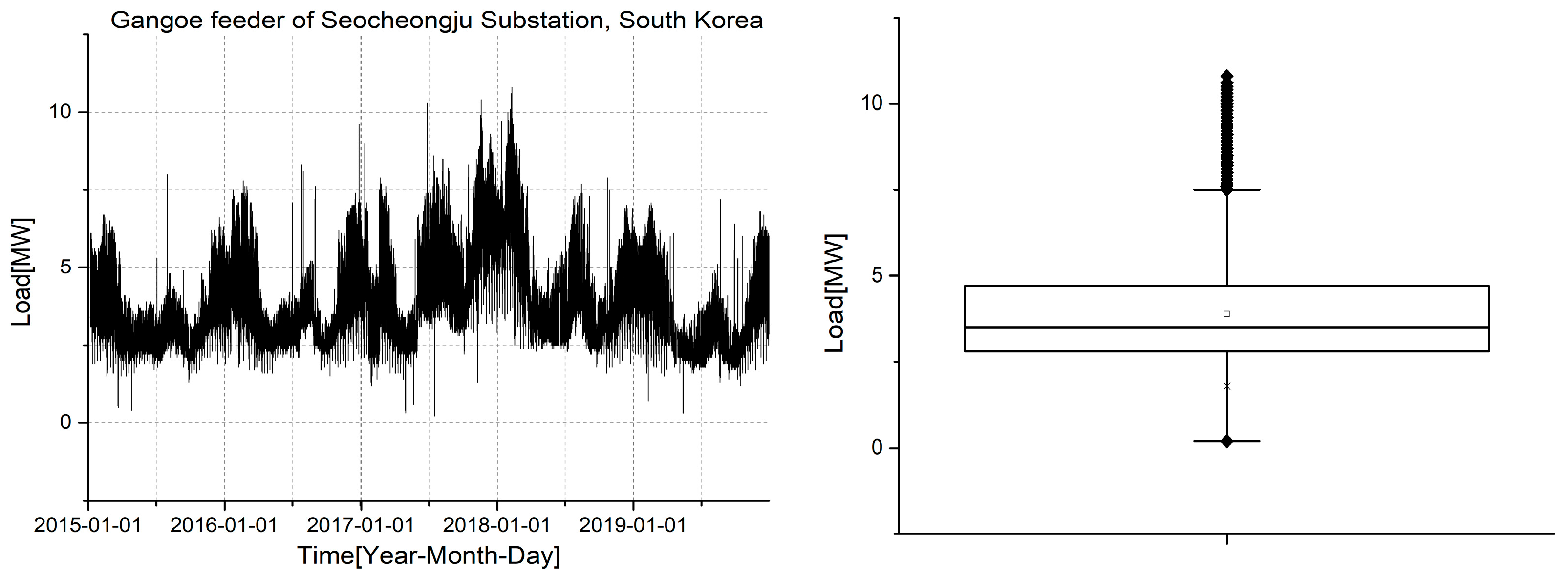
Figure 1. Time series and boxplot of hourly load data from the Gangoe feeder.
Energies 18 05385 g001
Figure 2. Schematic diagram of the proposed forecasting procedure.
Energies 18 05385 g002
Figure 3. Multi-resolution DWT analysis of Gangoe feeder load.
Energies 18 05385 g003
Figure 4. Load prediction result of Gangoe feeder: proposed model.
Energies 18 05385 g004
Figure 5. Load prediction result of Gangoe feeder: LSTM model.
Energies 18 05385 g005
Figure 6. Load prediction result of Gangoe feeder: Autoformer model.
Energies 18 05385 g006
Figure 7. Load prediction result of Gangoe feeder: NLinear model.
Energies 18 05385 g007
Figure 8. Boxplot comparison and error analysis: (a) actual vs. predicted feeder load distributions; (b) absolute error distribution of the proposed model.
Energies 18 05385 g008
Table 1. Comparison results with other forecasting models.
ModelMAE [MW]MAPE [%]RMSE [MW]Huber Loss [MW]
Proposed0.577117.72980.76060.2567
Autoformer0.939233.67071.12460.5286
LSTM0.725825.66510.89940.3514
NLinear0.583718.62950.79730.2702
Disclaimer/Publisher’s Note: The statements, opinions and data contained in all publications are solely those of the individual author(s) and contributor(s) and not of MDPI and/or the editor(s). MDPI and/or the editor(s) disclaim responsibility for any injury to people or property resulting from any ideas, methods, instructions or products referred to in the content.