Article

Bend–Twist Coupling for Small Wind Turbines: A Blade Design Methodology to Enhance Power Generation

by
Juan Pablo Vanegas-Alzate
1,
María Antonia Restrepo-Madrigal
1,
José Luis Torres-Madroñero
2,
César Nieto-Londoño
1,2,*,
Germán Alberto Barragán de los Rios
1,
Jorge Mario Tamayo-Avendaño
3,
Julián Sierra-Pérez
4,
Joham Alvarez-Montoya
2 and
Daniel Restrepo-Montoya
2,5
1
Grupo de Investigación en Ingeniería Aeroespacial, Universidad Pontificia Bolivariana, Medellín 050031, Colombia
2
Grupo de Energía y Termodinámica, Universidad Pontificia Bolivariana, Medellín 050031, Colombia
3
Grupo de Investigación e Innovación Ambiental, Departamento de Mecánica, Institución Universitaria Pascual Bravo, Medellín 050034, Colombia
4
Corporación Rotorr, Universidad Nacional de Colombia, Cr. 45 26-85, Bogotá 111311, Colombia
5
Facultad de Ciencias Empresariales, Corporación Universitaria Remington, Cl. 51 51-27, Medellín 111321, Colombia
*
Author to whom correspondence should be addressed.
Energies 2025, 18(20), 5353; https://doi.org/10.3390/en18205353
Submission received: 1 September 2025 / Revised: 6 October 2025 / Accepted: 8 October 2025 / Published: 11 October 2025

Abstract

Small-scale wind turbines (SWTs) represent a promising solution for the energy transition and the decentralization of electricity generation in non-interconnected areas. Conventional strategies to improve SWT performance often rely on active pitch control, which, while effective at rated conditions, is too costly and complex for small systems. An alternative is passive pitch control through bend–twist coupling in the blade structure, which enables self-regulation and improved power generation. This work proposes a novel blade design methodology for a 5 kW SWT that integrates passive bend–twist coupling with conventional pitch adjustment, thereby creating a hybrid passive–active control strategy. The methodology encompasses the definition of aerodynamic blade geometry, laminate optimization via genetic algorithms combined with finite element analysis, and experimental characterization of composite materials. Aerodynamic–structural interactions are studied using one-way fluid–structure simulations, with responses analyzed through the blade element momentum method to assess turbine performance. The results indicate that the proposed design enhances power generation by about 4%. The study’s originality lies in integrating optimization, structural tailoring, and material testing, offering one of the first demonstrations of combined passive–active pitch control in SWTs, and providing a cost-effective route to improve efficiency and reliability in decentralized renewable energy systems.

1. Introduction

The energy transition involves a shift in electricity generation from fossil fuels (i.e., oil, coal, and natural gas) to clean energy systems [1,2,3]. The energy transition effort worldwide is driven by the facts of environmental pollution and climate change, which are deepened by the intense use of fossil resources that dominate the energy market, accounting for approximately 73% of greenhouse gases (GHGs) [4]. Large-scale actions such as the Paris Climate Agreement 2012–2015, the 2030 Agenda adopted by the United Nations, and the 26th Conference of the Parties (COP26) are the most representative in achieving this energy transition. The Paris Agreement has as one of its pillars the development of new technologies to displace the transformation of energy from polluting sources, thus reducing CO2 emissions by 2030. The 2030 Agenda proposes goals and targets for sustainable development, encompassing social, economic, political, and environmental aspects. The COP26 (held in 2021) establishes climate change as a priority, emphasizing the achievement of carbon neutrality in all countries and regions [5].
In this sense, the study of renewable energies has been promoted, highlighting their competitiveness with traditional energy sources, depending on the location and available resources. These energy systems have gained increased applicability in recent years, with wind energy being a notable example [6]. In particular, small wind turbines (SWTs) offer energy transition solutions for decentralized systems where grid connection is not feasible [7] or non-interconnected areas [8] where diesel plants currently meet the load [9].
However, the design of SWTs faces a complexity balance in terms of efficient operation and suitability for various environments [10]. Particularly, SWTs are placed in unfavorable wind conditions, such as low ground clearance and terrain obstacles that limit wind speed and cause turbulence [11,12]. In this regard, aerodynamic design strategies and different control approaches have been explored to improve SWTs [13,14]. In practice, SWTs are often installed in suboptimal wind environments, characterized by low ground clearance and the presence of terrain obstacles that reduce wind speed and increase turbulence [11,12].
To address the challenges posed by suboptimal wind conditions, different aerodynamic design strategies and control approaches have been developed to improve the performance of small wind turbines. Among these, the most common control methods are stall and pitch control. The stall control system is often preferred in SWTs due to cost and nacelle space limitations as it allows manufacturers to avoid implementing a blade pitch mechanism, thereby reducing installation expenses [15]. However, this approach typically compromises the aerodynamic design of the blades, resulting in lower annual energy production (AEP) and limiting peak performance to maintain smooth energy regulation above the rated wind speed. Conversely, pitch control actively adjusts the blade angle to regulate the rotational speed, optimizing the turbine’s performance according to the wind resource at the operating site [15]. In this sense, it functions as an aerodynamic control strategy that modulates power output by altering the rotor’s aerodynamic behavior [16]. While pitch control enables enhanced power regulation and performance, it can also influence the structural loads acting on the turbine, either reducing or increasing them depending on the operating conditions [14].
There are two primary methods for implementing pitch control: active and passive. Active pitch control regulates the pitch angle of the blades actively, i.e., by a mechanism that rotates the blade, thereby adjusting the response of the wind turbine rotor to the existing wind conditions [17]. This mechanism can be integrated into a feedback control system [18]. The high costs of active pitch control systems [14] have compelled many small-scale turbines to adopt a fixed pitch control methodology, resulting in a suboptimal power regulation effect. The use of fixed blades is a primary technical disadvantage compared to large-scale horizontal wind turbines, which include active pitch control strategies to improve performance [19]. Meanwhile, passive pitch control only depends on the blade structure and the aerodynamic load on the blade [16,18].
One approach to enhancing rotor energy capture and reducing loads through passive pitch control is the use of rotor blades with bend–twist coupling. This concept has been numerically investigated to induce a passive torsional response in the blades, with Maheri et al. [20] reporting increases in annual energy production (AEP) of up to 13%. Similarly, Nicholls-Lee and Turnock [21] observed AEP gains of 2.65% for a rotor incorporating variable pitch and curvature. Notably, several studies have focused on large-scale turbines in the megawatt range; for example, Barr and Jaworski [22] reported a 14% increase in AEP for a 5 MW rotor. Passive bend–twist coupling incorporates several technologies for torsional blade actuation, including composite anisotropy, as demonstrated in aeroelastic and structural design work by Capuzzi et al. [23,24,25]. Recently, Tamayo-Avendaño et al. [26] employed a fluid–structure analysis in ANSYS 2023 R1 to evaluate the behavior of bending–torsional coupling in wind turbine blades, finding that the blade structure successfully undergoes torsional deflection along its longitudinal axis in response to an aerodynamic load, resulting in a 3% increase in annual energy production considering a wind resource with a Rayleigh distribution at an average speed of 11 m/s, an increase achieved without compromising key aspects of the technology, such as costs and structural integrity.
The use of pitch control is not only aimed at increasing generation power but is also used for load reduction. Some studies, such as the research by Sun et al. [27], have analyzed and optimized load reduction in large-scale wind turbine blades, explicitly focusing on the 15 MW IEA blade model. The methodology encompassed the introduction of bend–twist coupling (BTC) load reduction parameters, geometric sweep change (GSC) in GXBeam software, calculation of blade aeroelastic loading using BEM theory, followed by obtaining the steady-state analysis model of the rotating blade. Additionally, in the context of small wind turbines, a two-part study by Papadakis and Condaxakis [28,29] analyzed the performance of flexible curved blades of a small-scale wind turbine for passive control, comparing them with rigid blades. The flexible blades limited maximum rotational speed and power at high wind speeds, started generating power earlier (4 m/s vs. 6 m/s), and showed stable output. The same work tested layered GFRP blades with fibers at 20°, which achieved quick startup, stable power between nominal and cutoff speeds, and safe shutdown, confirming the effectiveness of passive regulation, although with a need for design refinement. Furthermore, Farias et al. [30] optimized the lamination sequence of a 660 W unidirectional composite blade to tailor BTC for passive load alleviation. Using BEM, ANSYS ACP/Fluent with two-way FSI, and surrogate models optimized via genetic algorithms, they constrained the axial displacement to 5% of the span length. The results showed that the torque increased by 8.3% compared to a spanwise unidirectional configuration. In comparison, the axial displacement remained below 3%, demonstrating that BTC-based tailoring is an effective passive pitch control strategy under overload conditions.
Given the complexity in the design of passive control by bend–twist coupling, some studies have opted for optimization techniques, such as Restrepo-Montoya et al. [31], who proposed a meta-model-based methodology to design laminates with a bend–twist coupling effect using genetic algorithms (GAs) and artificial neural networks (ANNs) integrated with a finite element model (FEA) capable of defining the stacking sequence that a laminate needs to reach a certain torsion angle when subjected to a bending load. This type of strategy resembles that of Herath et al. [32], who used a GA approach to optimize the composite layout in a morphing blade with differential stiffness element-induced bend–twist coupling. In other cases, the application of GA was used in the joint design of rotor geometry and structures by taking global parameters such as the AEP or the levelized cost of energy (LCOE) as the objective function of the optimization exercise [33,34,35]. Techniques that decrease the computational cost for performing a bend–twist coupling analysis have also been evaluated. Babuska et al. [36] developed a method involving the stiffness matrix (SMM) to analyze composite blades with bend–twist coupling, comparing it with commercial finite element models and analytical solutions. The technique proved to be accurate and versatile, enabling the efficient prediction of structural behavior in composite blades. The coupling resulted in a significant reduction in blade stiffness. Modal shapes and vibration frequencies were also significantly affected by coupling, and the analysis shows that correct predictions of natural frequencies are crucial due to their significant impact on operation.
Other studies have examined the integration of passive and active control to enhance wind turbine performance while mitigating structural loads. In this approach, blades are designed to rotate with flexure, thereby reducing the effective wind loads and lowering the demand on collective pitch actuators. For instance, Hayat and Ha [37] investigated bend–twist coupling (BTC) in a 5 MW wind turbine blade, showing that it can reduce fatigue loads and decrease the reliance on active pitch actuators. Their results indicated that the effectiveness of active pitch control decreased as BTC increased. However, this effect diminished at higher wind speeds due to the reduced torsional deformation induced by the bending of the blades. Similarly, Zahle et al. [38] demonstrated numerically that combining passive–active pitch control in large rotors can effectively relieve loads, with active blade pitch used to enhance energy capture below rated wind speeds and to alleviate structural loads above the rated range. Manolas et al. [39] extended this line of research by analyzing passive and active load control methods on the DTU 10 MW Reference Turbine, showing that, while BTC alone reduced flapwise fatigue loads by about 7%, the greatest alleviation (≈30%) was achieved when combined with active strategies such as Individual Pitch Control (IPC) and Individual Flap Control (IFC). These works, however, focused on large-scale turbines, an idea supported by the conclusions of relatively recent studies such as [40]. In contrast, the integration of passive–active hybrid pitch control in small wind turbines remains understudied, which underscores the novelty and relevance of the present study.
The previous passive–active pitch control strategy has not been extensively studied for small wind turbines, and even the concept of using passive–active control to increase generation, which is ideal for small wind turbines, is not evident in the literature. For all the above reasons, this study proposes assessing the blade design of a 5 kW small wind turbine, incorporating passive pitch control using bend–twist coupling, and its effect if the pitch angle is actively changed from cut-in operation to nominal operation. For this purpose, this study addresses the blade design for passive–active control, considering aerodynamic and geometric design, material characterization, and the design of composite laminates. The resulting blade design is evaluated using a one-way numerical fluid–structure simulation to assess the aerodynamic and twist behavior; then, a post-processing BEM model is used to determine the performance improvements by the passive–active control. In this sense, in Section 2, this article presents the methodology of each design stage (aerodynamic geometry, material characterization, laminate design, and numerical approach); in Section 3, the results obtained from the blade design are presented and discussed for fifteen typical operating cases that characterize the power–wind speed curve.

2. Methodology

This section presents the blade design methodology for the small wind turbine, as illustrated in Figure 1. The process is divided into three main stages: (1) the aerodynamic design of the rotor, (2) the composite laminate design, and (3) the material characterization. The methodology begins by determining the aerodynamic and geometric configurations of the blade, utilizing blade element momentum (BEM) modeling combined with an optimization approach for rotor geometry and airfoil selection. Following this, the composite material is experimentally characterized. Then, the laminate design of the constructive composite material is addressed, which involves the classical lamination theory (CLT) alongside a finite element model (FEM), integrated with a genetic algorithm (GA) optimization to define the optimal fiber orientation in the laminates. The outputs from these three stages are used to finalize the blade design, which is then assessed through a one-way numerical fluid–structure integration (FSI). Finally, the blade’s performance is evaluated using the BEM modeling. The flowchart also specifies the computational tools employed at each stage of the design process. Each application is described in detail below.

2.1. Rotor Aerodynamic Design

The rotor performance, as well as the analysis of the relationships between the involved parameters, can be achieved through different mathematical models, each with varying degrees of sophistication, computational cost, and detail. For this study, the methodology proposed from an aerodynamic perspective consists of analyzing the rotor’s aerodynamics using the BEM and vortex filament method (VM); these models will be used to estimate the blade geometry configuration [41]. The implementation of these two models usually results in low computational costs as the fidelity of the obtained results is high relative to the required computational time [42]; moreover, these models are usually used in preliminary calculations and integrated with additional modules that allow the analysis of other disciplines, such as aeroelasticity.

2.1.1. Blade Element Momentum Formulation

Blade element momentum (BEM) theory relies on an actuator surface approach to rotor loads, as described by Hansen [42], and is a highly popular tool in wind turbine aerodynamic analysis [43]. The BEM model is built on the definition of rotor loads from both momentum and blade element modeling but involves a degree of empirical data, including separately measured or estimated airfoil coefficients and an empirical correction for rotor loading at specific operating conditions. This approach has proven to be reliable and less computationally demanding compared to robust analysis methods, such as full CFD approaches. BEM is also a widely used option for assessing the performance of horizontal-axis wind turbines (HAWTs). The simplicity of this model stems from its foundation on two simplified models that describe the interaction between the turbine rotor and the air it captures. The force that the flow applies to the rotor is modeled as the change in linear and angular movement of the flow between two points, upstream and downstream from the rotor. This theory, known as momentum theory, models the turbine’s rotor as an actuator disk that extracts energy from the flow passing through it.
The flow behavior over a finite surface, such as the wind turbine blades, differs significantly from the flow over an infinite surface. On a turbine blade, the free end creates a pressure differential over the top and lower surfaces, which generates tip vortices that produce drag and reduce the blade’s overall efficiency, affecting its performance and altering both the lift and stress distribution along the blade. The flow behavior phenomena are not considered when defining the BEM model, mainly because the blade lift and drag coefficients are usually obtained from experimental data collected from tests with two-dimensional models [42]. For this reason, the BEM model is generally corrected with the losses at the tip of each blade, which are initially attributed to Prandtl.
The correction for finite wing is performed using the Prandtl factor F defined as [44]
F = 2 π arccos e f ,
with f defined as a function of the radial position r over the blade,
f = B ( R r ) 2 r sin φ ,
R being the rotor external radius and φ the flow angle [44].
The Prandtl correction factor affects both the thrust and torque; in this sense, the expressions of the BEM model for differential thrust and torque are
d T = 4 π r ρ V 2 a ( 1 a ) F d r ,
d M = 4 π r 3 ρ V ω ( 1 a ) a F d r ,
V is the free stream velocity, ω is the rotor angular velocity, ρ is the air density, and a is the axial induction factor. Rotor blade rotation transfers some kinetic energy into the flow, which is modeled in terms of the tangential induction factor a and is related to the induced axial velocity u 1 and flow velocity through the rotor u, according to the velocity triangle shown in Figure 2, where ω is the rotational velocity, α l is the local angle of attack, θ is the pitch angle; F n , F t a n , F a e r o , L, and D are the normal, tangential, aerodynamic, lift, and drag forces, respectively.
Another correction that must be applied to the BEM model is known as the Glauert correction for highly loaded rotors, which adjusts the thrust coefficient when the axial induction factor exceeds its threshold of 1 / 3 , corresponding to Glauert’s original model. This correction can be expressed as [44]
C T = 4 a ( 1 a ) F x 1 / 3 4 a 1 1 4 ( 5 3 a ) a F x > 1 / 3 ,
where the thrust coefficient is defined as a function of the thrust force and differential disk element with area d A [45]:
C T = 2 d T ρ V 2 d A .
The BEM theory enables the description of the various forces acting on a differential section of the blade as a function of dynamic pressure ( 1 / 2 ρ V r e l 2 ) and characteristic length (c). Aerodynamic force coefficients in two dimensions associated with the element, C l and C d (lift and drag coefficients), depend on the section local angle of attack α l and local Reynolds number R e . In this regard, aerodynamic forces can be expressed as having a normal component to the plane of rotation F n and another force parallel to the plane F t as follows:
F n = 1 2 ρ V r e l 2 c C n ,
F t = 1 2 ρ V r e l 2 c C t ,
where C n and tangential C t force coefficients can be determined by knowing C l ( R e , α l ) and C d ( R e , α l ) , which are the section two-dimensional aerodynamic coefficients; these can be obtained via experimental results or numerical simulations. The relation between these sets of coefficients can be represented through an axis rotation related to the flow angle of the section φ :
C n = C l cos φ + C d sin φ ,
C t = C l sin φ C d cos φ .
This way, the BEM theory enables establishing a new definition for both thrust and torque differentials acting over each discrete element, taking into account that each actuator disk element with area d A corresponds to B discrete elements associated with a B number of blades, following
d T = B F n d r ,
d M = r B F t d r .
The BEM model implementation is centered around the iterative calculation of axial a and tangential a induction factors from an initial assumption. The MATLAB routine implemented for this project (see Figure 3) evaluates the convergence of both induction factors by calculating the L 2 norm. The convergence criterion is set at a tolerance of 1 × 10 6 to obtain a solution in approximately 90 iterations. The BEM model assumes that a rotor blade can be divided into consecutive elements, each located at a specific distance from the rotor center and independent of the others. In this way, the distribution of mechanical loads acting on the rotor is determined by calculating the thrust force (perpendicular to the rotor plane), the product of the tangential force, and the radius of each element. The distribution of axial and tangential loads is input for the mechanical analysis of the rotor. The integration of the tangential loads to the rotor radius is used to calculate the power extracted by the turbine. The validation process of the BEM model applied in this study is presented in Appendix A.1. Additionally, the process of obtaining the optimal blade geometry is shown in Appendix B.

2.1.2. Airfoil Selection

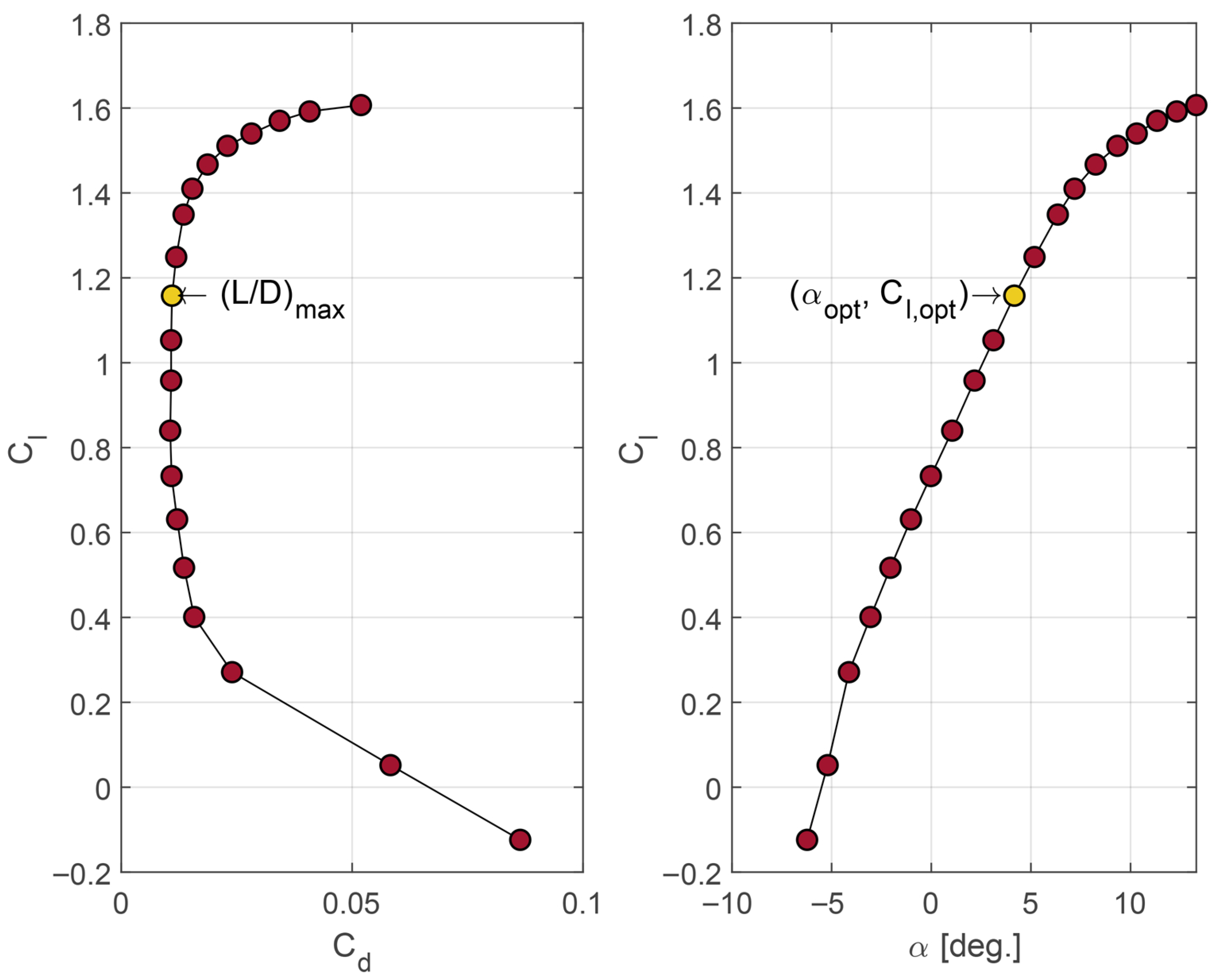
Airfoil selection is conducted by prioritizing the optimal rotor operation condition. Airfoil selection criteria can be divided into quantitative and qualitative criteria. Quantitatively, according to the BEM model [42], the tangential force coefficient that contributes to torque generation is maximized when the lift-to-drag ratio is maximized C l / C d ; this occurs when C l , o p t , C d , o p t , and α o p t are achieved. Assuming aerodynamic optimality is the design criterion, the optimal angle of attack and corresponding coefficients become the input for estimating optimal chord and twist distribution along the blade. A series of airfoil characteristics are included in Giguère and Selig’s study on airfoils for wind energy applications [46]. Two airfoils have been adopted from that work, with the L / D ratio serving as the primary criterion. A simple analysis is presented for two selected airfoils and shown in Figure 4 and Figure 5, which contain two plots, each illustrating the aerodynamic efficiency of the S822 and SG6043 airfoils, respectively. The first plot in each figure shows the maximum aerodynamic efficiency when the lift-to-drag ratio ( C l / C d ) reaches its peak, that is, when lift is maximized and drag is minimized. The second plot illustrates the variation in the lift coefficient with respect to the angle of attack, indicating an optimal angle of attack at which the lift-to-drag ratio is highest.
On the other hand, considering the qualitative selection criteria, airfoil selection is based on its intrinsic characteristics and their relation to optimal rotor operation, such as sensitivity to leading-edge roughness and behavior of the lift coefficient in the stall region. This design procedure takes into consideration L / D as well as airfoil thickness, aiming for a sufficiently stiff geometry without the need for internal structural elements. This requirement is particularly important for designing small wind turbines, in which simplicity is key. As a result, the S822 and S823 airfoils are considered here due to the relatively large thickness ratio compared with other geometries in [46].

2.2. Material Characterization Methodology

This study aims to utilize experimentally obtained data from the characterization of carbon fiber composites to optimize the ply stacking sequence based on classical lamination theory (CLT). The primary objective of this optimization is to achieve bend–twist coupling for use as a passive control system in a wind turbine blade. Three mechanical tests were conducted to obtain the necessary material properties: tensile, compression, and shear testing. The resulting data will then be used to calculate the material properties, which will serve as input for a genetic algorithm designed to optimize the stacking sequence of unidirectional carbon fiber plies, ensuring improved aerodynamic efficiency and energy capture.

2.2.1. Tensile Properties’ Characterization

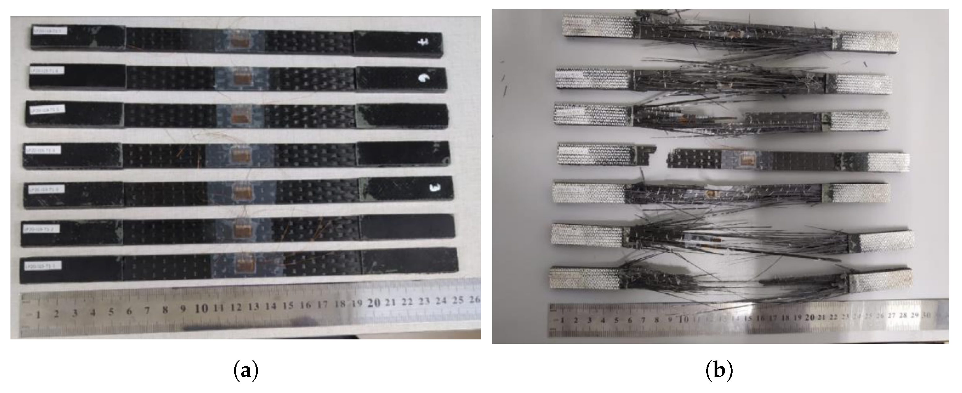
Tensile testing was conducted based on ASTM D3039/D3039M—17 [50] Standard Test Method for Tensile Properties of Polymer Matrix Composite Materials and ASTM D638—22 [51] Standard Test Method for Tensile Properties of Plastics. The tests are performed by placing a thin flat strip of material with a constant rectangular cross-section into the grips of a mechanical testing machine. A tensile load is then applied at a steady rate until failure, while the applied force is continuously recorded to determine the ultimate tensile strength. To evaluate the stress–strain behavior of the specimen, strain gauges are attached, allowing calculation of the tensile modulus of elasticity, ultimate tensile strain, Poisson’s ratio, and transition ratio.
The test specimens (Figure 6) were manufactured according to the ASTM standards, with tabs at the end of the test specimen to ensure minimal slip during testing. Seven test specimens with different fiber orientations were manufactured, each one having tabs at the end. The reinforcement consisted of high-strength carbon fiber with a filament diameter of 7 μ m and fiber density of 12 K. As a matrix, a low-viscosity infusion epoxy system was employed, providing rapid fiber wet-out and a glass transition temperature up to 92 °C after post-curing. Strain gauges were located at the midpoint of the test specimen to ensure accurate strain readings. The tensile test specimen had a total length of 175 mm, a width of 25 mm, and a thickness of 2 mm. Tabs with a length of 25 mm and a thickness of 2 mm were attached to the gripping ends to ensure proper load transfer and prevent premature failure. The test was conducted at a load rate of 3 mm/min ±25% with a strain rate of 0.1 mm/mm until failure. The universal testing machine (UTM) monitored the force applied throughout the test until failure. With this test, the ultimate tensile strength, ultimate tensile strain, Poisson’s ratio, transition strain, and moduli of elasticity were determined. At the same time, the specimen was anticipated to exhibit a fiber-dominant failure mode, such as fiber breakage or fiber–matrix debonding, which is standard in carbon fiber-reinforced composites under tensile loading.
From the measured failure load ( F f ) and the strains in the principal directions ( ε 1 , ε 2 , and ε 3 ) the tensile strengths, elastic moduli in each direction, and Poisson’s ratios were derived using Equations (13), (14), and (15), respectively [50]:
σ i = F f A c h , i ,
E i = d σ i d ε i ,
ν i j = ε j ε i ,
where i denotes the direction of the applied load (e.g., 1, 2, or 3), j is the perpendicular direction in which the lateral strain is measured, and A c h , i is the cross-sectional area normal to the load at i direction.

2.2.2. Compressive Properties’ Characterization

Compressive testing was conducted based on ASTM D695-15 Standard Test Method for Compressive Properties of Rigid Plastics [52]. The test is performed by placing a standardized test specimen between two compression platens in a mechanical testing machine and applying a compressive load until failure while monitoring stress–strain behavior via strain gauges placed on the test specimen. The main objective of this test is to calculate the compressive modulus of elasticity, ultimate compressive strain, and ultimate compressive strength. Although ASTM D695 was designed with rigid plastics in mind, its methodology can be applied to fiber-reinforced polymer matrix composites, such as carbon fiber epoxy laminates [52]. Seven test specimens were also manufactured with different fiber orientations and placed into specially designed fixtures to ensure that failure occurred inside the calibrated area.
The compression test specimen (Figure 7) had a total length of 80.77 mm, a width of 12.7 mm, and a thickness of 1.02 mm, with a gauge length of 4.78 mm. The test was performed at a load rate of 1.3 mm/min ± 25%, applying a compressive force until specimen failure occurred. The UTM continuously monitored the applied force and deformation throughout the test, and tabs were used at the specimen ends to ensure proper load distribution and prevent premature crushing at the grips. This test determined the ultimate compressive strength, ultimate compressive strain, Poisson’s ratio in compression, and compressive modulus of elasticity. At the same time, the specimen was anticipated to exhibit a failure mode such as fiber buckling, interlaminar shear failure, or crushing, which are typical in carbon fiber composites under compression. From the measured failure load F f , the ultimate compressive strength in each direction was derived using Equation (13), considering that the exact formulation applies for both tensile and compressive strengths [52].

2.2.3. Shear Properties’ Characterization

Shear testing was conducted based on ASTM D5379-D5379M-19 [53] Standard Test Method for Shear Properties of Composite Materials by the V Notched Beam Method. The test enables the calculation of shear strength, shear modulus, and strain, critical properties for characterizing anisotropic materials, such as carbon fiber-reinforced composites. The test specimens were manufactured in accordance with ASTM D5379/D5379M-19, with seven specimens produced having different fiber orientations. Two strain gauges were placed on each specimen to monitor flex due to the applied shear force. The shear test specimen had a total length of 76 mm and a width of 11.4 mm. The notch depth was 3.8 mm, with a notch root radius of 1.3 mm. The overall specimen height was 19 mm, and the thickness ranged from 3 to 4 mm, as required, while the tab thickness was 1.5 mm. The test was conducted with a head displacement rate of 2 mm/min and a shear strain rate of 0.01 min 1 until failure. Two shear strain gauges were placed along the test section to measure the shear strain accurately during testing, spanning the length between the notch roots.
This test determined the shear stress response, ultimate shear strength, ultimate shear strain, and shear chord modulus of elasticity. Depending on the laminate configuration and fiber orientation, the specimen was expected to fail through in-plane shear fracture at the notch or interlaminar delamination. From the measured failure load F f and the strain in the 45° direction ε 45 , the shear stress and the shear modulus of elasticity for different material planes were determined using Equations (16) and (17) [53].
τ i j = F f h b ,
G i j = τ i j γ i j ,
where h is the distance between the notches, b is the specimen thickness, τ i j is the shear stress, G i j is the shear modulus of elasticity, and γ i j is the shear strain, all defined for the corresponding material plane.

2.3. Composite Laminate Design

The proposed methodology for the laminate design consists of two stages. The first one consists of the creation and validation of a finite element model (FEM) that can simulate the bend–twist coupling and apply it to both a carbon fiber-reinforced polymer plate (CFRP) and a simplified model of the rotor blade (see validation process in Appendix A.2). The second stage involves using a genetic algorithm coupled with the created FEM model to determine the correct stacking sequence of the laminate that achieves the developed twist angle of the blade.

2.3.1. Classical Lamination Theory (CLT)

Classical lamination theory establishes that, depending on the stacking sequence of a laminate, it can exhibit coupling effects between axial and angular deformations, allowing designers to create structures that utilize coupled deformation effects to enable the “intelligent” change of a structure [21]. For the coupled phenomena to exist in the laminate, specific values in the stiffness matrix have to be different from zero. In this regard, Equation (18) represents extensional stiffness and coupling terms for extension–extension ( A 12 ) and extension–shear ( A 16 and A 26 ).
N x N y N x y = A 11 A 12 A 16 A 12 A 22 A 26 A 16 A 26 A 66 ϵ x ϵ y γ x y + B 11 B 12 B 16 B 12 B 22 B 26 B 16 B 26 B 66 κ x κ y κ x y M x M y M x y = B 11 B 12 B 16 B 12 B 22 B 26 B 16 B 26 B 66 ϵ x ϵ y γ x y + D 11 D 12 D 16 D 12 D 22 D 26 D 16 D 26 D 66 κ x κ y κ x y ,
The terms B i j correspond to membrane stiffness and flexure–extension coupling, while D i j represent bending stiffness and flexure–torsion coupling ( D 16 and D 26 ). For a laminate to exhibit flexure–torsion coupling, the terms D 16 and D 26 must be non-zero [54]. In the above equation, x and y are the laminate central axes in longitude and width, respectively; N x , N y , and N x y are normal forces applied to the laminate in those directions; M x , M y , and M x y represent the applied moments on the laminate in their respective orientations; ϵ x and ϵ y represent the mid-plane linear deformations; κ x , κ x and κ x y are curvature deformations on the laminate; and γ x y are angular deformations because of shear.
The values that comprise the stiffness matrix depend on the mechanical properties of the lamina that create the laminate and the different fiber orientations of the reinforcement fibers in each layer, as shown in Equations (19)–(21). In these, N is the total number of layers in the laminate, Q i j are the values of the reduced stiffness matrix of the lamina, Q ¯ i j represent the values of the transformed reduced stiffness matrix, which depend on the angles of the reinforcement fibers of the lamina ( α ) for the laminate coordinate system, and z k is the distance of the lamina from the mid-plane of the laminate. Further, 1 is the lamina direction parallel to the fiber orientation, 2 the perpendicular direction to 1 throughout the width of the lamina, and 3 the normal orientation to the 1 2 plane. In Equation (21), E 1 and E 2 are the lamina elasticity modules in 1 and 2, respectively, ν 12 and ν 21 are the Poisson ratios of each lamina that composes the laminate in planes 1 2 and 2 1 , respectively, and G 12 is the shear modulus on the 1 2 plane of the lamina.
A i j = k = 1 N Q ¯ i j k z k z k 1 , B i j = 1 2 k = 1 N Q ¯ i j k z k 2 z k 1 2 , D i j = 1 3 k = 1 N Q ¯ i j k z k 3 z k 1 3 .
Q ¯ 11 = Q 11 cos 4 ( α ) + 2 ( Q 12 + 2 Q 66 ) sin 2 ( α ) cos 2 ( α ) + Q 22 sin 4 ( α ) , Q ¯ 12 = ( Q 11 Q 22 4 Q 66 ) sin 2 ( α ) cos 2 ( α ) + Q 12 ( sin 4 ( α ) + cos 4 ( α ) ) , Q ¯ 22 = Q 11 sin 4 ( α ) + 2 ( Q 12 + 2 Q 66 ) sin 2 ( α ) cos 2 ( α ) + Q 22 cos 4 ( α ) , Q ¯ 16 = ( Q 11 Q 12 2 Q 66 ) sin ( α ) cos 3 ( α ) + ( Q 12 Q 22 + 2 Q 66 ) cos ( α ) sin 3 ( α ) , Q ¯ 26 = ( Q 11 Q 12 2 Q 66 ) sin 3 ( α ) cos ( α ) + ( Q 12 Q 22 + 2 Q 66 ) cos 3 ( α ) sin ( α ) , Q ¯ 66 = ( Q 11 + Q 22 2 Q 12 2 Q 66 ) sin 2 ( α ) cos 2 ( α ) + Q 66 ( sin 4 ( α ) cos 4 ( α ) ) .
Q 11 = E 1 1 ν 12 ν 21 , Q 12 = ν 12 E 2 1 ν 12 ν 21 , Q 22 = E 2 1 ν 12 ν 21 , Q 66 = G 12 .

2.3.2. Laminate Design Genetic Algorithm

Once the methodology for the numerical simulation of rotor blade bend–twist coupling has been established, the next step is to describe how this coupling can be effectively utilized. In this work, a genetic algorithm (GA) is used to design the optimal laminate stacking sequence. The GA is a stochastic algorithm whose search process resembles the natural phenomena of gene inheritance that occur during evolutionary processes. These algorithms analyze the genetic information of individuals in a predetermined population, guiding genetic exchange and mutation until an individual with the desired genetic makeup is found [55]. The proposed GA in this project has the stacking sequence of the blade’s skin as the dependent variable and the mechanical properties of the blade, along with the rotation angle ( ϕ ), as the independent variables, with ϕ defined as the objective. Each chromosome represents a possible stacking sequence, and each gene corresponds to the fiber orientation of its respective layer. The chromosomes must meet the following conditions:
  • The stacking sequences must be symmetrical, odd, and unbalanced to generate only the bend–twist coupling effect.
  • The fiber orientation angle represented in each gene ( α ) must be an integer value between –90° and 90°.
  • There cannot be more than four consecutive plies with the same orientation angle.
  • Every layer of the laminate must have the same thickness.
The GA operation integrates two different software programs. The algorithm is programmed in MATLAB R2020, while the evaluation of individual fitness is performed using the FEM previously described with ANSYS APDL [56]. Given the hollow composition of the wind turbine blade and the small thickness of the laminates, the structural stiffness matrix is expected to change after each deformation step; for this reason, the present analysis relies on a non-linear model based on the procedures proposed by Newmark [57] and Hilber et al. [58]. The finite element formulation corresponds to a shell-type element, characterized by a negligible thickness compared to the transverse dimension, as stated by [59]; this is a key characteristic for many composite structures. In ANSYS APDL [56], the formulation corresponds to the SHELL181 element with six degrees of freedom, based on the First-Order Shear Deformation theory, also known as Mindlin–Reissner Shell theory [60,61], which assumes small changes in curvature for a given time increment.
The FEM model serves as the core of an iterative procedure that encompasses criteria beyond structural response. Specifically, one part of the iterative GA cycle is developed in MATLAB, while the other is created in ANSYS. First, the mechanical properties of the composite material laminate to be used on the blade skin are defined. Then, the load acting on one of the faces of the blade is specified, along with the desired rotation angle at the blade’s free end (target). Once the GA defines this input information, it generates the initial population to begin its iterative search process. Given the high computational cost of each fitness evaluation with GA–FEA coupling, a moderate population size of 20 randomly generated individuals was selected to balance exploration and computational expense [62,63]. These individuals are formed by a chain of 11 genes, each with a value corresponding to the fiber orientation angle of the respective layer. In this way, a stacking sequence [0/−30/+65/−50/+90/−45] is encoded as a vector [0° −30° 65° −50° 90° −45° 90° −50° 65° −30° 0°].
Once the initial population is generated, the individuals must be evaluated by ANSYS APDL. To enable interaction between the two software packages, a MATLAB script was created to store the necessary commands in an array to run the FEM program in ANSYS APDL. This array is then written into a plain text file (.txt), which can be read as input by ANSYS. The information that is passed to ANSYS APDL from these files includes the following:
  • The mechanical properties of the composite material laminates used, specifically the Young’s modulus in the three principal directions ( E 1 , E 2 , and E 3 ), the Poisson’s ratio in the three planes ( ν 12 , ν 23 , and ν 31 ), the shear modulus in the three planes ( G 12 , G 23 , and G 31 ), and the laminate density ( ρ l ).
  • The laminate thickness (t).
  • The magnitude of the load acting on the blade face.
From MATLAB, the system command is executed to open ANSYS APDL in batch mode, providing each created file as input. ANSYS APDL runs the FEM with the supplied information and outputs the rotation produced on the free end face of the blade ( ϕ ), storing each result in a .txt file that MATLAB can use as input for the GA next step. Once MATLAB obtains the rotation results for each individual, the parent selection process is carried out by choosing the 10 chromosomes with the best fitness, meaning those that achieved a rotation closest to the defined target. The deterministic tournament method was used for parent selection, a category of elitist methods that aim to select only the best-fitting members of the population, in contrast to proportional methods that allow every individual a chance to be chosen, even those with poor fitness. The advantage of using an elitist method is that it converges in fewer iterations, meaning it reaches a solution faster and consumes fewer computational resources [64].
The 10 parents undergo the crossover recombination, producing 10 new child chromosomes. Due to the elitist nature of the parent selection method, the two-point recombination method was selected [65]. The GA randomly determines the positions of both cut points, which are the same for all chosen parents. The cut segments are then exchanged between the parents to produce the chromosomes of the offspring. Although some GA–FEA optimization studies employ mutation probabilities between 1 and 5% [66], this work adopts a rate of 10% for all offspring genes, which is justified by the use of a relatively small population and the high computational cost of the objective function in the FEA model, maintaining genetic diversity and avoiding premature convergence [67]. This process is fundamental in enriching the genetic diversity of the new population, thereby increasing the GA’s search capability. The chromosomes of the 10 parents and the 10 offspring are combined to form a new population of 20 chromosomes. The GA then continues iterating through the evaluation, selection, recombination, and mutation processes until a population gives rise to an individual that produces a rotation close to the target, with a difference of less than 5%. The optimization process by GA is illustrated in the flowchart in Figure 8.

2.4. Fluid–Structure Simulation

The one-way fluid–structure integration (FSI) methodology combines the geometry obtained from aerodynamic design, material characterization, and composite laminate design. The blade geometry is entered into ANSYS-Workbench, integrated with the domain geometry in Fluent for CFD numerical analysis. The same geometry is also used in the ANSYS Composites PrePost (ACP) module to define the laminate design. Finally, the pressure loads obtained from CFD, the laminate design from ACP, and the composite properties are imported into a steady-state analysis in ANSYS Mechanical, where the properties obtained from the material characterization are entered; this is conducted to verify that the in-operation twist distribution along the blade span meets the design targets under the expected aerodynamic and inertial loads.

2.4.1. Fluid Domain and Formulation

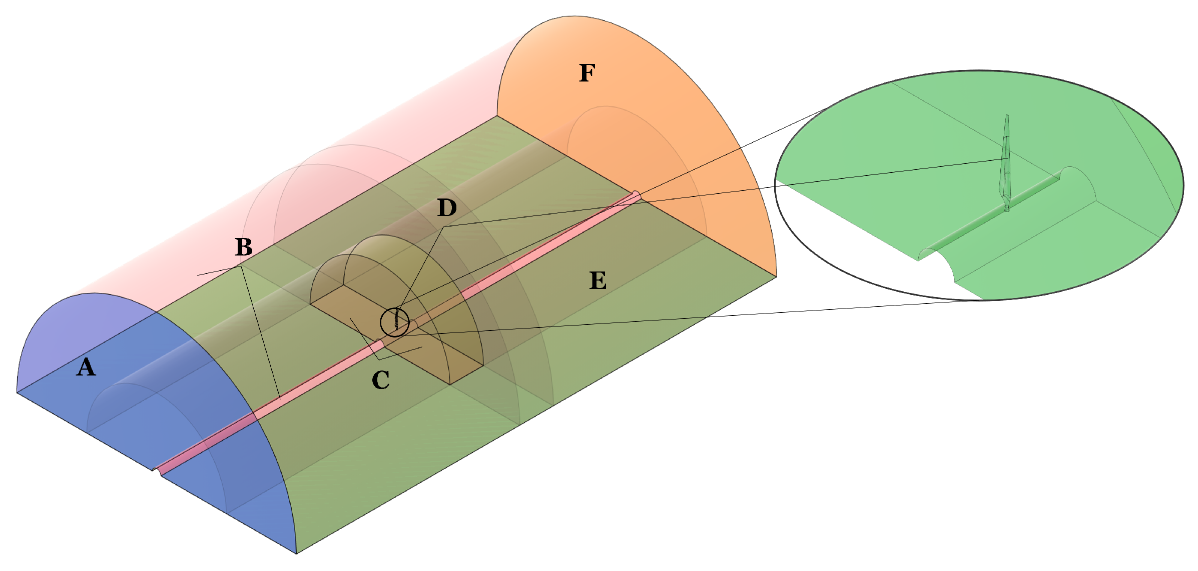
The fluid-flow solver employs a steady-state pressure-based formulation of the Reynolds-averaged Navier–Stokes (RANS) equations together with the k ω SST turbulence model. To reproduce the blade’s operating conditions while minimizing computational cost, a rotational-periodicity approach is adopted: the fluid domain is shaped as a semi-cylindrical volume whose cross-sectional area matches that of the NASA Ames wind tunnel test section (i.e., 24.4 m × 36.6 m). Periodic boundary conditions are imposed on two planes separated by 180°, labeled “E” and “C” in Figure 9. This domain setup follows Tamayo-Avendaño et al. [26], who based their configuration on the experimental work of Hand et al. [68] and the numerical validation by Sørensen and Johansen [69] for the NREL Phase VI blade.
The outer cylindrical boundary of the main flow domain (face “B” in Figure 9) has a radius of 16.86 m and extends 28.96 m both upstream and downstream from the rotor plane. The inner cylindrical surface, also labeled “B”, has a radius of 0.508 m, matching the blade root radial location. A separate sliding (rotating) subdomain, bounded by the faces marked “D”, is defined with an outer radius of 8.43 m and an axial width of 2.03 m. To eliminate wall friction effects, symmetry boundary conditions are applied to all inner and outer cylindrical surfaces (collectively “B”). A velocity inlet is specified at the upstream plane “A”, and a pressure outlet is applied at the downstream plane “F”. The solution of the pressure–velocity coupling is performed using the explicit SIMPLEC scheme, which allows the fine-tuning of under-relaxation factors to control the convergence and stability of the numerical solution. The meshing process includes an inflation zone that is applied with 12 prism layers, a 20 % growth rate, and a first-layer height of 4 × 10 5 m . This setup yields y + 1.15 , which is sufficient for boundary layer resolution. The rest of the domain is meshed with hexahedral elements to reduce computational cost, following the methodology employed by Tamayo-Avendaño et al. [26]. The mesh for the domain is shown in Figure 10a, and the inflation between the blade wall and the domain is illustrated in Figure 10b.

2.4.2. Composite Structural Simulation

The blade’s structural response is evaluated using a steady-state finite element analysis (FEA). Aerodynamic loads are imported as external pressure fields from a steady-state CFD simulation in a one-way coupling configuration. The pressure distribution computed on the blade surface is mapped onto the structural mesh in the static mechanical model to perform a stress and deformation analysis. This approach avoids the computational cost of an iterative fluid–structure system coupling loop while still capturing the aerodynamic loading effects on the blade surface. Following the methodology of Lee et al. [70], the mapped pressure is treated as a static load on the structure. The structural model also includes centrifugal effects from the prescribed rotational speed and the blade’s self-weight.
To accurately represent the blade’s composite construction, the ANSYS ACP (Pre) module is used to define the material’s anisotropy and the properties of the layers. The orthotropic properties of each lamina (ply), including elastic moduli, shear moduli, and Poisson’s ratios in principal material directions, are determined along with the laminate layup. Stacking sequence, fiber orientation angles, and ply thicknesses (see Figure 11a) are specified within ACP (Pre), ensuring that each shell element in the mesh has the correct local ply orientations and through-thickness material properties. Such detail is essential for capturing structural behaviors such as bend–twist coupling. In ACP (Pre), the blade geometry is linked to the ply definitions, stacking sequences, and reference coordinate systems. The fully defined composite data is then exported and integrated into the static structural module.
The wind turbine blade is modeled with 42 , 698 triangular and quadrilateral SHELL181 elements (see Figure 11b) using a characteristic element size of 7.5 mm. This mesh density was chosen to facilitate laminate definition and meshing in ACP (Pre). This element formulation is based on the First-Order Shear Deformation Theory (also known as the Mindlin–Reissner theory), which incorporates transverse shear deformation, critical for accurately modeling composite structures. Wind turbine blades often feature thick root sections where shear deformation is significant; the Mindlin–Reissner approach allows the model to capture these shear strains accurately. Unlike thin-shell formulations, SHELL181 does not enforce the Kirchhoff–Love assumption, enabling the representation of both bending and shear couplings through the thickness. This is particularly important in load-sensitive regions such as the blade root and tip, where accurate modeling of these effects is essential for structural integrity assessment.

3. Results and Discussion

This section presents the results underpinning the blade design workflow. First, steady-state aerodynamic analyses were used to define and refine the blade geometry. Second, material characterization informed the laminate stacking sequence. Third, the laminate and geometry were assessed via a one-way CFD-to-structural workflow, from which twist distributions were recovered across various operating conditions. Finally, these twist distributions were propagated into a BEM model to quantify the impact of the laminate design on power production and blade loads.

3.1. Rotor Aerodynamics

The calculation of the optimal geometry was performed at a single operating point ( λ = 7.48 ) for a turbine with a rotor diameter of 5 m, which corresponds to the typical size of a horizontal-axis wind turbine with a nominal power range of 2 kW to 5 kW. For simplification purposes, the S822 airfoil is used across the entire blade cross-section. For this airfoil, the optimal operating point occurs at an angle of attack α opt = 5.9 ; at this angle, the aerodynamic efficiency ( C l / C d ) reaches its maximum value with C l and C d values of C l = 0.86 and C d = 0.013 .
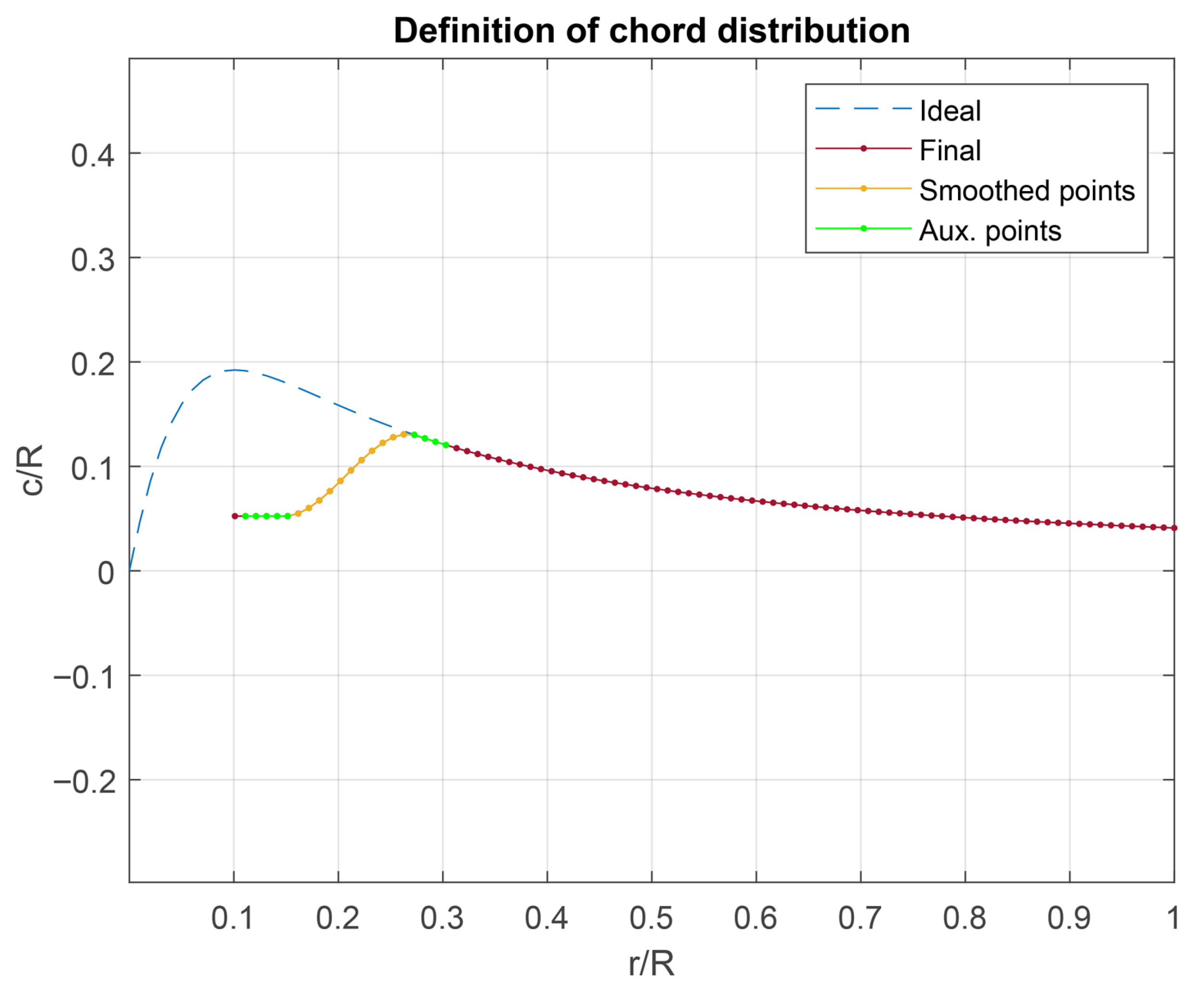
The ideal geometry results correspond to both the chord c and twist β distributions along the blade, as seen in Figure 12. Assuming the joining element between the blades and the rotor axis, called hub, has a diameter equivalent to 12% of the rotor diameter, the chord distribution is limited until the end of the hub, as shown in the results. Additionally, the maximum chord is truncated at a point equivalent to 26% of the radius. The blade segment between 12% and 26% is designed to provide sufficient structural support to the rest of the blade. The chord distribution along this section of the blade was defined using cubic interpolation, as shown in Figure 13. Auxiliary segments were built to create the interpolation function around the transition point. Under the same design premise, it can be observed that the distribution of β is truncated for r / R 0.26 , precisely because, in this region, the blade’s cross-section serves a structural rather than an aerodynamic function.

3.2. Results of Material Characterization

For the carbon fiber samples in the material characterization process, the results of force applied as a function of deformation from the tensile, compression, and shear tests are shown in Figure A5 in Appendix C, yielding the results summarized in Table 1. Based on these experimental results, it was possible to determine the elastic properties of the material, including the Young’s modulus in different directions, Poisson’s ratios in various planes, and shear moduli, as presented in Table 2 and Table 3.
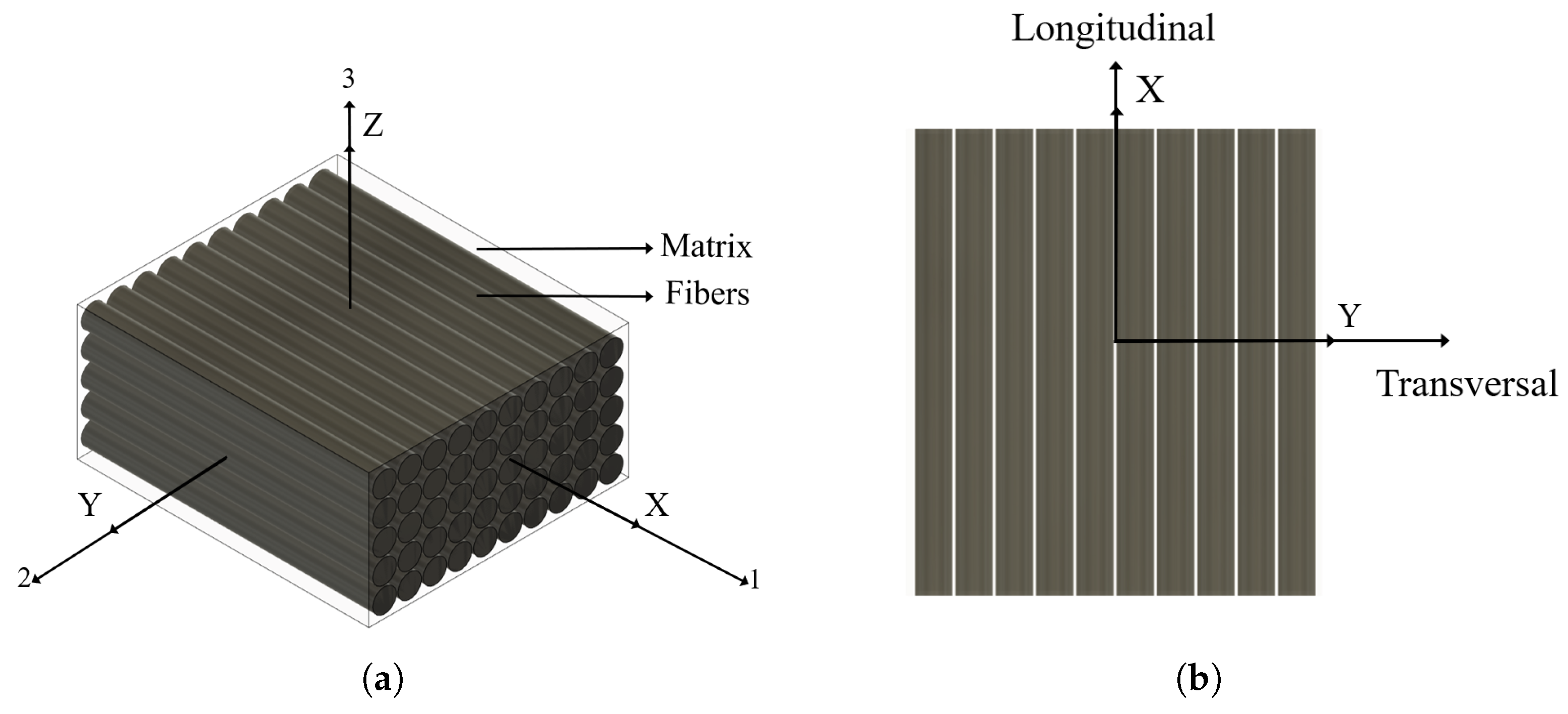
Table 1 presents the average values of maximum load ( F max ) and maximum stress ( σ max ) obtained from tensile, compressive, and shear tests performed on the carbon fiber composite. The results reveal pronounced anisotropy in the mechanical behavior of the laminate. In tension, the longitudinal direction (as shown in Figure 14b) exhibited a significantly higher strength, reaching an average of 1.98 GPa . In contrast, the transverse direction showed a much lower value of only 0.022 GPa . A similar trend was observed in compression, with longitudinal strength reaching 0.26 GPa , compared to 0.11 GPa in the transverse direction. In the shear test, performed along the 1–2 direction (as shown in Figure 14a), the average maximum stress was 0.075 GPa . It is worth noting that no shear test was conducted in the 2–3 direction.
Table 2 presents the average elastic properties obtained from tensile and compression tests on carbon fiber composite specimens. It is observed that the longitudinal elastic modulus E 1 is slightly higher under compression (28.22 GPa) compared to tension (26.08 GPa), which could be attributed to improved load transfer along the fiber direction under compressive loading. The transverse modules E 2 and E 3 also varied with the loading mode, both reaching 9.12 GPa in compression and 6.26 GPa in tension, which is consistent with the orthotropic behavior of the laminate and reflects the sensitivity of the transverse response to loading type. Poisson’s ratios ν 12 and ν 13 remained nearly constant in both tests (both 0.337 in tension and 0.340 in compression), while ν 23 showed more variation (0.370 in tension vs. 0.311 in compression), possibly due to the compressibility of the matrix system in the transverse plane.
On the other hand, Table 3 shows the average shear moduli of the composite material, corresponding to directions G 12 , G 31 , and G 23 . The shear modulus obtained from the Iosipescu shear test along the fiber plane was 1.44 GPa. This property defines the in-plane shear stiffness of the reinforced laminate. The modulus G 23 was not obtained experimentally but was estimated from the technical datasheet of the epoxy resin used as the matrix in the composite, resulting in a value of approximately 1.18 GPa. The properties calculated here were used to parameterize the composite material used in ANSYS ACP (Pre).

3.3. Laminate Design

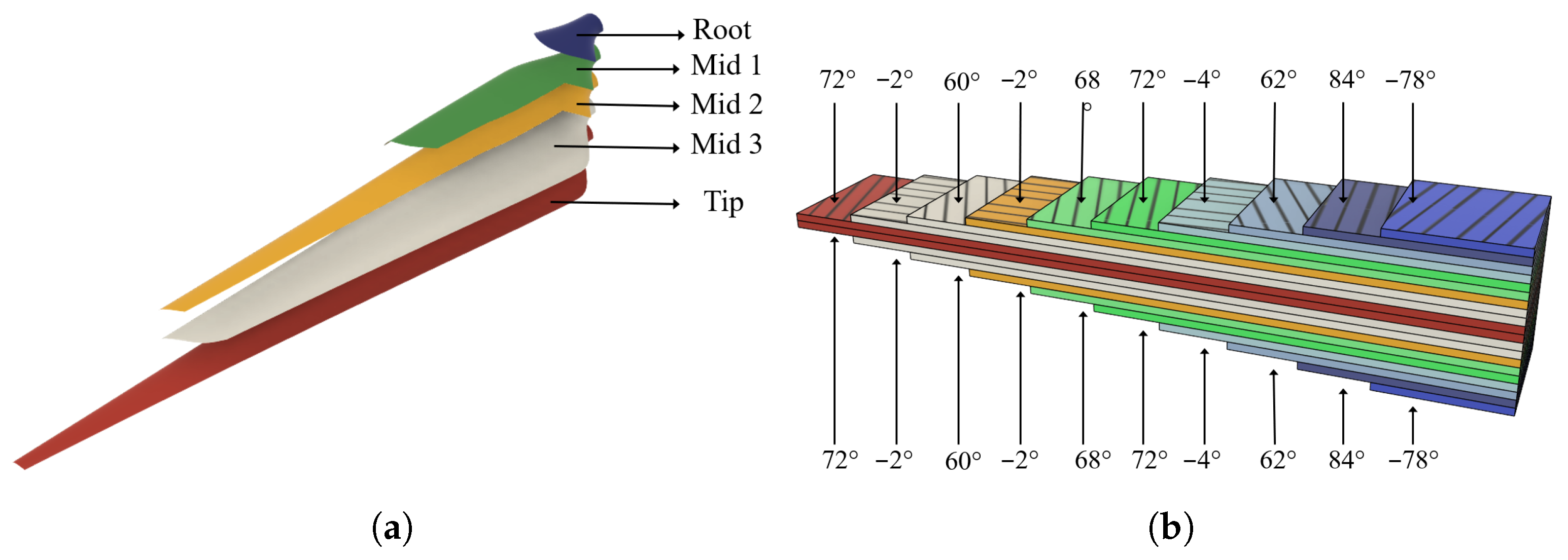
The results obtained from the rolling sequence when applying the genetic algorithm described in Section 2.3 are shown in Table 4. The blade laminate design consists of two main stages. First, the ply cut patterns and their placement on the blade surface were defined through an iterative process, targeting thicker laminates towards the leading edge of the blade to promote the desired twist distribution shown in Figure 15a. Second, the ply orientations and stacking sequence were specified (see Figure 15b) to maximize the effectiveness of the passive control system while maintaining the required structural stiffness and aerodynamic performance.
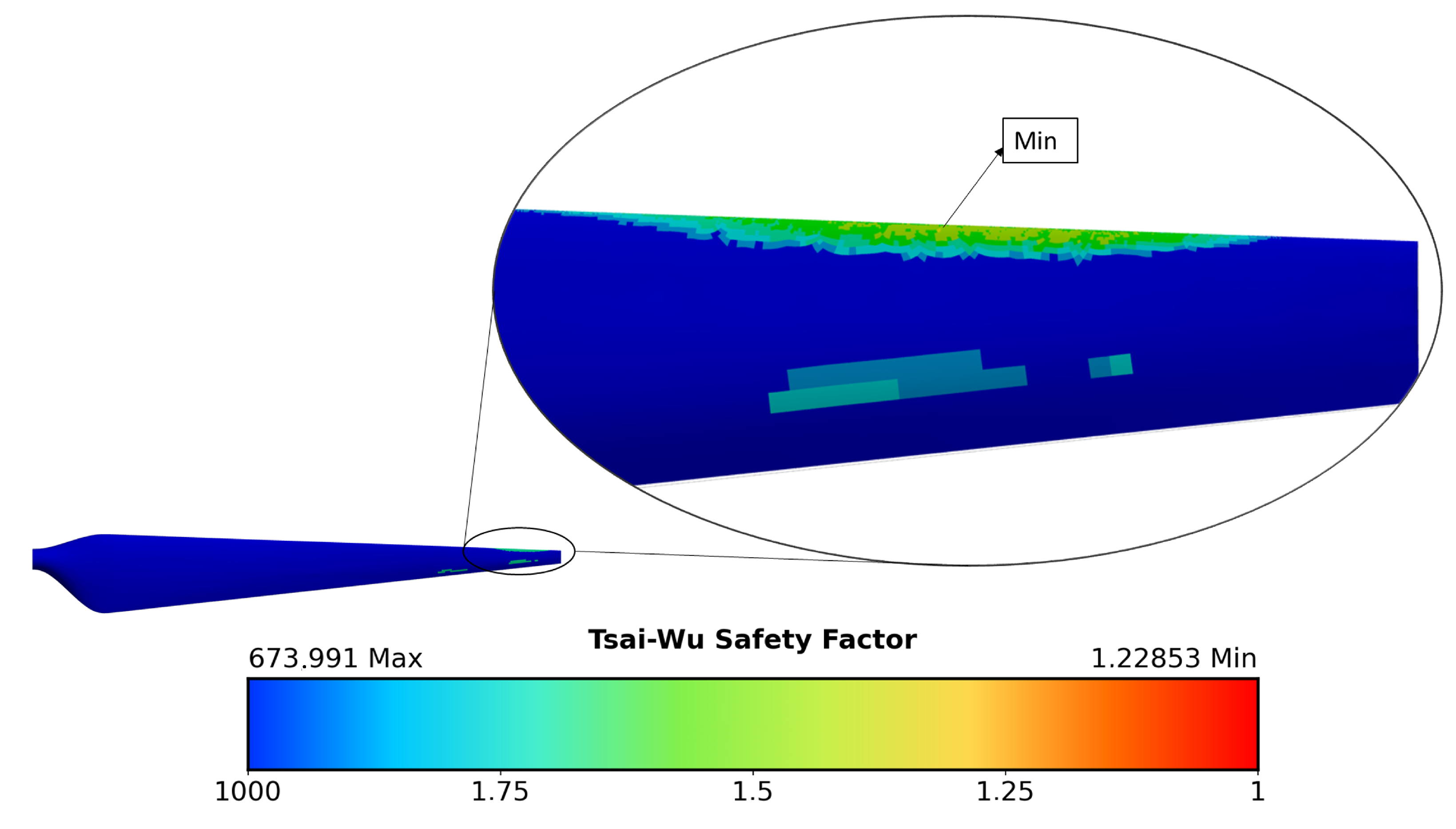
To ensure the safe operation of the turbine blade, a composite failure analysis was carried out using the Tsai–Wu criterion. This approach accounts for the anisotropic properties of the material, the interaction between stress components along different axes, and the distinction between tension and compression, which is an essential consideration since composites are typically weaker in compression [71]. Moreover, the Tsai–Wu criterion evaluates multiaxial stress states, providing a more realistic prediction of failure under complex loading conditions [72]. These features make it particularly suitable for the failure analysis of wind turbine blades [73]. The study was performed at cut-out conditions (see Table 5) using the composite failure criteria tool in ANSYS Mechanical. A global assessment of the blade was conducted, followed by a local evaluation at the extrados tip ply (see Figure 15), where the lowest safety factor was observed. This result was expected as the blade region is predominantly subjected to compressive loads, which are inherently weaker in composite structures. At this operating condition, the minimum safety factor reached a value of 1.22 , as shown in Figure 16. The relatively low safety factor of 1.22 occurs under cut-out conditions, which represent an extreme and infrequent operational scenario. During normal operation, the margin remains higher.
Furthermore, the leading-edge reinforcement applied during manufacturing strengthens the extrados–intrados junction, mitigating local compressive failure and delaying fatigue mechanisms such as delamination. Regarding manufacturing variability, typical defects such as fiber misalignment, resin-rich regions, or voids can locally reduce strength. However, the safety factor reported here is a conservative estimate obtained from nominal properties. In practice, quality control standards for composite blades (e.g., ply orientation tolerance and bonding inspections) help to ensure that variability remains within limits that do not compromise long-term operation.

3.4. Simulation Results

The geometry resulting from Section 3.1, the characterization of the composite material in Section 3.2, and the laminate design of Section 3.3 constitute the comprehensive design of the 5 kW wind turbine blade. These elements serve as the inputs for the numerical modeling process, where the mechanical properties identified during material characterization are incorporated. It is important to note that the mechanical behavior of the material is intrinsically related to the manner in which the lamination process is carried out during blade manufacturing. To represent the blade’s operational regime, five simulation campaigns were conducted with a total of fifteen different simulations: the first at cut-in, with the blade set to −9° relative to the rotor rotation plane. This initial setting is achieved via the active control system to produce the required cut-in torque. Once the rotor is underway, the active control returns the blade to 0 , at which angle the passive load-alleviation mechanism is most effective. Furthermore, this consideration is taken into account because, below the rated speed, it is not necessary to vary the pitch angle as the wind turbine should produce as much energy as possible; meanwhile, at high wind speeds, active pitch control can be used to prevent excessive mechanical energy production and limit the generated energy to the rated level [74]. It is under these conditions that integrated passive–active pitch control behavior will be studied. There are three additional campaigns in the optimal operating range at 9 m/s, 15 m/s, and 21 m/s and a final campaign at the cut-out speed of 30 m/s. In each case, three simulations were run with an increment of ± 1 m / s to obtain a clear picture of the blade’s behavior in and around the corresponding operating conditions. The cases are listed in Table 5.

3.4.1. Aerodynamic Simulation

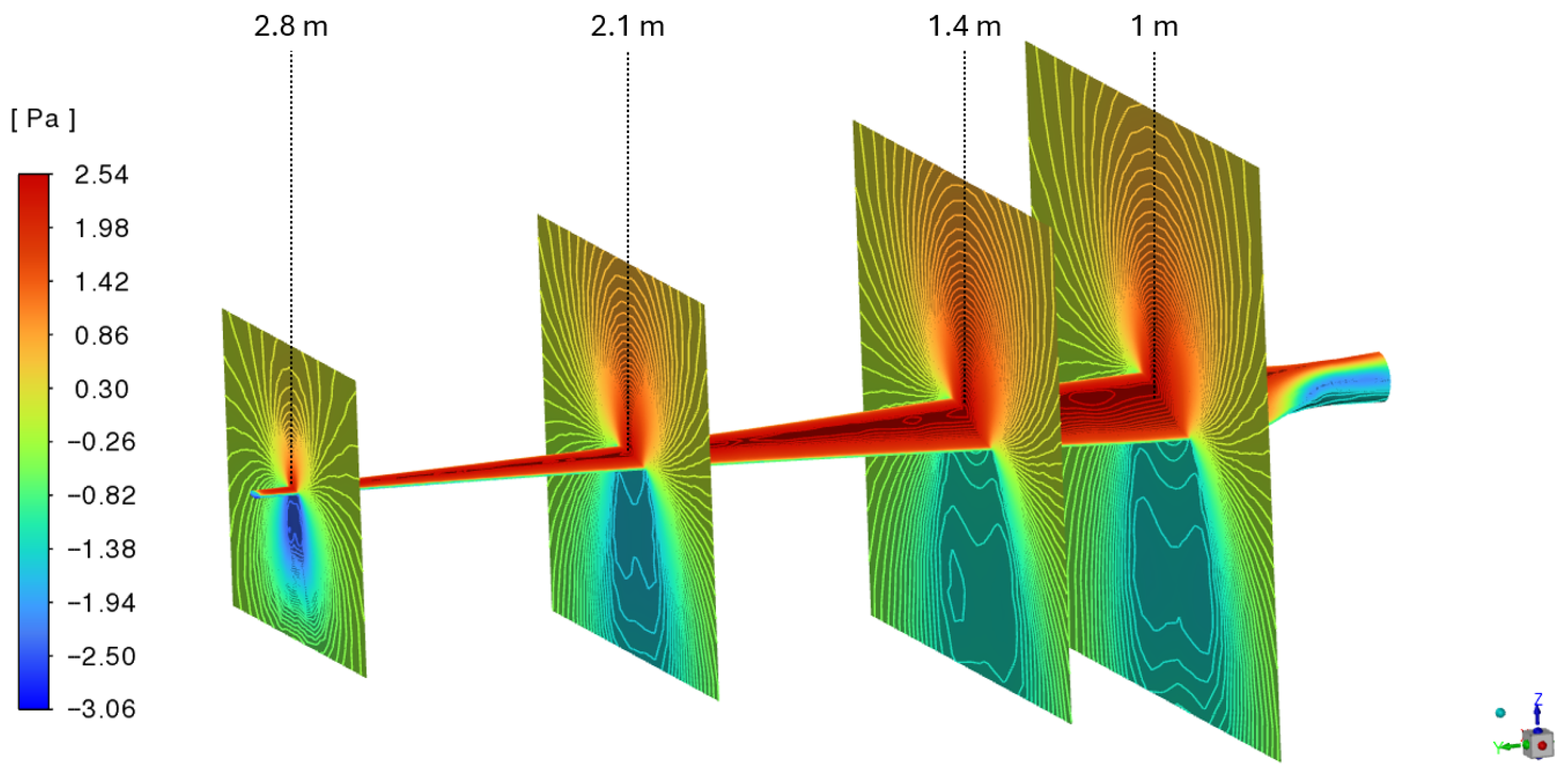
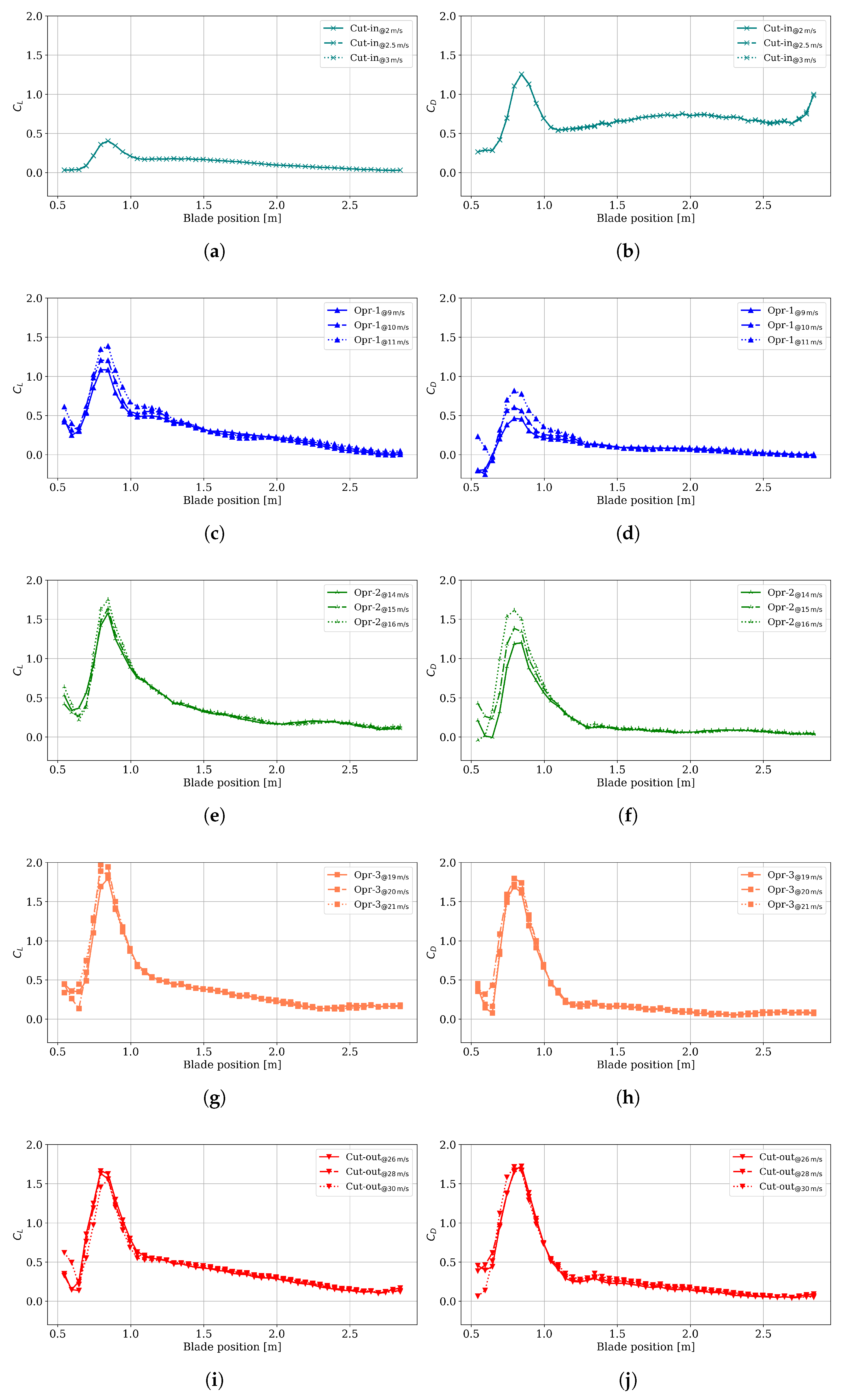
The primary objective of the steady-state CFD simulation is to obtain the static–pressure distribution on the blade surface; Figure 17 provides the pressure contours for the cut-in operation at 2 m/s, 0 rpm, and −9° of angle of attack. Similarly, the pressure contours were imported into the structural model to perform stress and deformation analyses. To represent the loads on the blade in the case studies, from the CFD results, nodal static pressure and wall shear stress are exported for post-processing to compute the lift and drag coefficients, C L and C D , along the blade surface, as indicated in Figure 18.
From the spanwise distributions of C L and C D on the blade surface, the expected trends are observed across all the operating conditions. The C L curve rises from the root, reaches an inboard peak, and then decreases toward the tip. This inboard peak is attributed to a higher effective angle of attack relative to the rest of the blade, as well as the thicker airfoil sections near the root, which were necessary to achieve the required structural integrity of the blade under critical conditions. The C D distribution exhibits a similar shape; at higher wind speeds, both baseline and peak values increase along the span (see Figure 18h,j). In some regions, the effective angle of attack exceeds the stall angle, resulting in separation and increased turbulence, which further increases the drag coefficient, C D . The resulting increase in normal aerodynamic load enhances the blade’s bend–twist coupling, improving its effectiveness, as discussed in the following section.

3.4.2. Blade Twist Variation

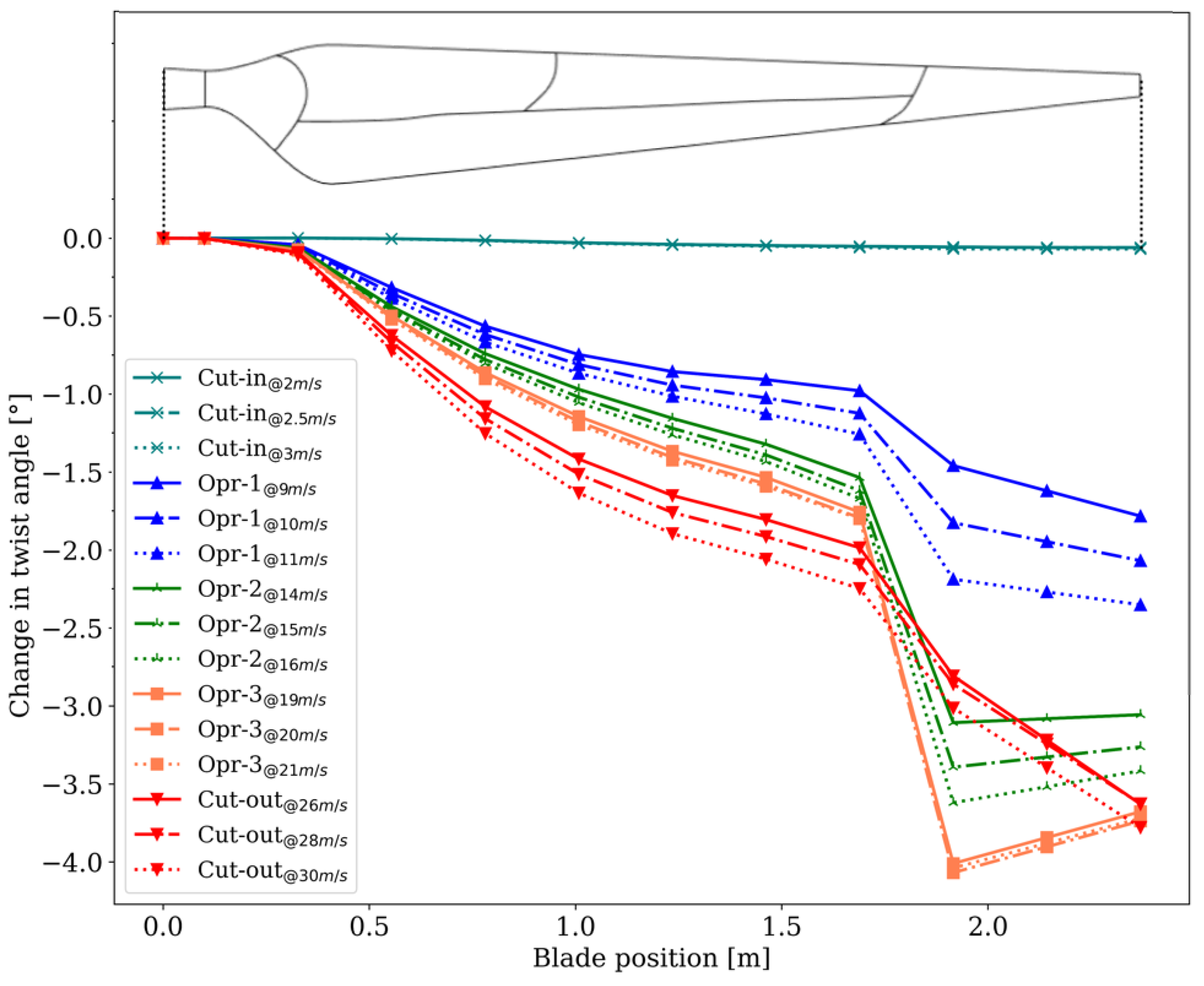
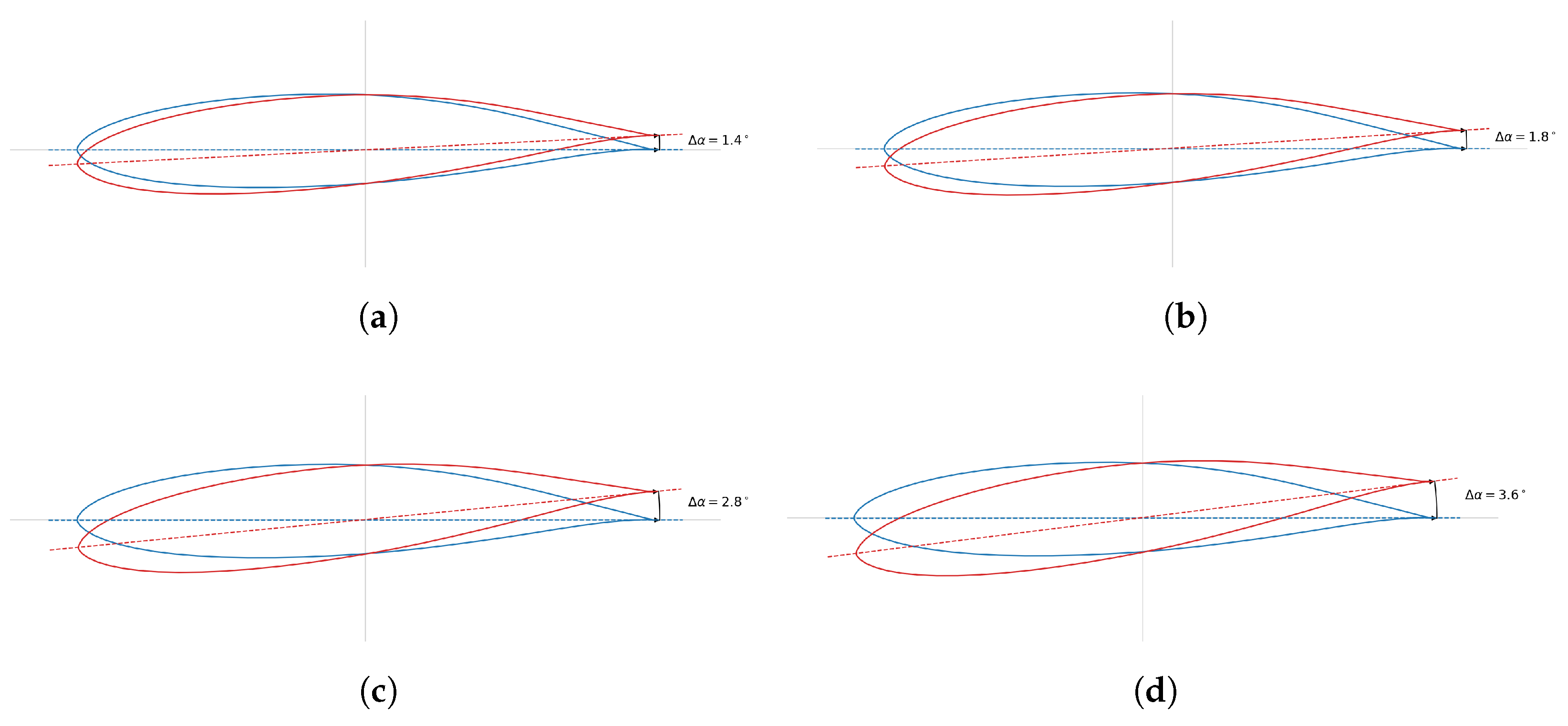
The twist evolution along the blade span due to aerodynamic forces is presented in Figure 19 for all the cases analyzed, reported in Table 5. Mechanical simulations revealed that twist increases under load as the carbon-fiber layup tapers toward the tip. At the highest operating speeds (Opr-3 and cut-out), local buckling in the thin tip region (see Figure 11a) further amplifies the twist response. This passive load-alleviation mechanism reduces the local angle of attack, thereby improving aerodynamic efficiency and ultimately increasing energy capture. The resulting twist distribution was subsequently exported and applied in a BEM analysis to quantify its influence on torque and power generation, enabling comparison with a purely rigid blade response. This effect is clearly observed in Figure 20, where variations in the local angle of attack induced by structural twist at specific locations (see Figure 21) of the blade are presented, highlighting the influence of thickness distribution along the blade. In particular, Figure 20d shows the local angle variation at the blade tip, where the laminate is thinnest and the flapwise bending moments are largest, conditions that enhance the effectiveness of bend–twist coupling. For the above, the twist results indicate that bend–twist coupling enables the blade to adapt to wind variability passively. At low to moderate speeds, the designed angle of attack is preserved for efficient energy capture. At high speeds, the twist reduces loads and delays stall, improving aerodynamic efficiency, which has a direct influence on energy capture.

3.4.3. BEM Results

By applying the twist distributions obtained from the composite structural simulations to the BEM model, it is possible to quantify the impact of the passive control system on blade loads and power production, which are critical aspects for the final output of the composite blade. The calculated angle of attack α l is provided in Figure 22, which shows that this decreases toward the tip because the local tangential speed ω r grows with radius, which reduces the inflow angle and thus α l . Compared with the rigid blade, the flexible blade shows a decrease in α across most of the span: flapwise bending under aerodynamic load induces elastic twist that effectively lowers the local pitch, and it is most noticeable near the blade tip region.
By applying the twist distributions obtained from the composite structural simulations to the BEM model, the influence of the passive control system on blade loads and power production can be quantified—two key factors determining the final performance of the composite blade. The calculated angle of attack, α l , is presented in Figure 22. As shown, α l decreases toward the blade tip because the local tangential speed ω r increases with radius, thereby reducing the inflow angle and consequently α l . In comparison with the rigid blade, the flexible blade exhibits a reduction in α along most of the span due to flapwise bending under aerodynamic loading, which induces an elastic twist that effectively decreases the local pitch, with the effect being most pronounced near the tip region.
The resulting C L (see Figure 23a) and C D (see Figure 23b) distributions differ significantly from those obtained with CFD (see Figure 18). This difference comes from the simplifications of the BEM model compared to the complete three-dimensional flow physics captured by CFD. For example, in BEM, the radial component of the airflow over the blade is assumed to be zero, an approximation that strongly affects the prediction of stall behavior. In reality, radial flow induced by rotation, together with centrifugal effects, delays stall and alters the effective lift and drag, a phenomenon only captured in CFD. Additionally, near the blade tip, both C L and C D diverge from CFD values because turbulence and vortex dynamics are not resolved in BEM. Instead, empirical tip-loss factors truncate the aerodynamic loading to approximate a realistic lift distribution; however, unlike CFD analyses, this treatment cannot replicate the detailed flow structures and pressure gradients that are relevant to rotor aerodynamics.
From the BEM analysis, the spanwise distributions of normal force F N (see Figure 24a) and tangential force F T (see Figure 24b) were obtained. These forces are critical for blade operation: F N , acting perpendicular to the rotor plane, is the primary contributor to flapwise bending moments and therefore strongly influences the bend–twist coupling that underpins the passive control system. The results indicate a spanwise reduction in F N at high wind speeds, most likely caused by a reduced blade incidence angle. Under these conditions, C L increases, whereas C D decreases by a relatively larger amount (see Figure 23). In contrast, F T acts parallel to the rotor plane and is directly responsible for torque generation and, consequently, power production. For the flexible blade, F T increases for wind speeds above 10 m/s, resulting in higher available torque and, consequently, increased rotor power. Because the angles of attack are reduced, as shown in Figure 22, the drag force is reduced to a greater extent than the lift. This situation is convenient for torque generation due to its higher L/D ratio and has a positive impact on rotor thrust. Additionally, the axial force components decrease at some higher wind speeds.
By updating the twist distribution using the data from Figure 19, the resulting differences in torque and thus power output can be evaluated. As expected from the increase in tangential loads (see Figure 24b), the power output (Figure 25a) exhibits a noticeable increment within the generator’s optimal operating range, demonstrating the effectiveness of the passive control system for power increase. Furthermore, the power coefficient curve (Figure 25b) remains well within the Betz limit for a horizontal-axis wind turbine. It shows an improvement at moderate wind speeds, confirming both the aerodynamic consistency of the results and the physical feasibility of the design. Rotor power is known to be a function of V 3 at the same time that the power coefficient depends on V 1 , which explains why bend–twist coupling seems to cause a disproportionate change between rotor power and power coefficient.
As shown in Figure 25a, the passive coupling control system yields an increase in rotor power output, reaching 982 W at higher wind speeds, which corresponds to an improvement of approximately 4 % in overall power generation due to a proportional increase in rotor torque (Figure 26b) at the blade’s optimal operating regime. Such an increment in rotor power occurs at almost the same level of thrust (Figure 26a), demonstrating no adverse effect on tower and foundation structural demands. At the same time, tangential forces decrease (see Figure 24b), normal forces increase (see Figure 24a), and, since the normal force component primarily drives thrust, the overall thrust remains nearly unchanged if not reduced for most wind speeds. Finally, the effectiveness of the proposed passive control system can be illustrated by assuming a Rayleigh probability density function as a model for the wind resource, with average wind speeds of 6, 8, and 10 m/s. In such cases, the effect of bend–twist coupling results in improved annual energy captures, by 3.9%, 9.7%, and 13.3% for each one of the assumed average wind speeds, and this corresponds only to mechanical power output. It must be noted that these figures are consistent with the reported improvements in the literature, as found by the review in [40], in which AEP increments from bend–twist coupling were registered to vary between 1.8% and 14% for large wind turbines (e.g, 5 MW or 10 MW) and for FSI analyses that do not include GA optimization. In a comprehensive system analysis, power output may be reduced due to system losses in electrical and mechanical components; however, the potential remains substantial if higher average wind speeds or more widely spread wind speed probability distributions are considered.

4. Conclusions

The primary objective of this work was to design a wind turbine blade incorporating a passive control system based on a smart composite laminate layup to assess the potential benefits and limitations of such a system in operation. The aerodynamic design was carried out for a turbine with a nominal power of 5 kW and a rotor diameter of 5 m . Although aerodynamic performance was the primary design criterion, structural considerations were also essential to ensure that the blade maintained sufficient stiffness while implementing the smart laminate. To achieve the appropriate laminate orientation for the bend–twist coupling mechanism, a material characterization campaign was conducted. This characterization provided the data required to calibrate the numerical model, which in turn guided the definition of the laminate stacking sequence forming the passive control system. One of the main challenges in defining the layup was not only to obtain the desired twist distribution but also to do so while preserving the structural integrity of the blade, particularly at higher wind speeds, where the passive control system is the most effective but the bending moments are also the largest. While the laminate orientation was optimized using a genetic algorithm, the ply cut patterns were defined iteratively to simplify the design process and maximize structural robustness.
Within the possibilities offered by the proposed methodology, it is reasonable to consider, under a sensitivity analysis framework, how the configuration of laminates can change with new forms of heuristic optimization or machine learning tools. Moreover, although the present study employed a one-way fluid–structure interaction (FSI) approach, the methodology proved robust by combining high-fidelity aerodynamic loading, detailed finite element modeling of the composite layup, and a validated multiaxial failure criterion (Tsai–Wu). This framework ensured that the critical structural responses of the blade were captured with sufficient accuracy across the operating envelope despite the absence of feedback from structural deformation to the aerodynamic field. Given that the blade deflections remained small relative to the chord length, one-way FSI represented a practical and reliable method of analysis. Nevertheless, extending the work to a two-way FSI formulation remains an essential avenue for future research, particularly in scenarios where aeroelastic coupling or large deformations are expected to play a more dominant role.
The comprehensive blade design methodology was evaluated up to the stage of a numerical model; however, one of the challenges posed, which is clearly promising, is the manufacture of the blade, where, by guaranteeing the properties of the composite material and the proposed geometry, it would be possible to evaluate the challenges in fiber orientation, resin matrix filling control, intrados and extrados adhesion, and the curing process, among others. Additionally, another future task would be the operational integration into a rotor that also involves an active control system, achieving the operational curves of power generated and C p . In this regard, although the 4% increase in AEP is in line with the order of magnitude reported by some studies, it may be the subject of future research, where evaluations are carried out under different wind conditions, or the effect of increasing the size and capacity of small wind turbines is studied.
Regarding the scalability of the improvement in AEP, it must be noted that, as long as the increase in blade twist is maintained, there should be a proportional response in power output since both angular displacement and aerodynamic coefficients are non-dimensional quantities. Nevertheless, the question of whether a larger blade would benefit from a bend–twist coupling approach remains open. On one hand, assuming a finite torsional response is reasonable for larger blades with similar structural configurations, but a rigorous estimation regarding the scalability of the improvement should include further numerical analysis so that the inevitable changes in blade stiffness are taken into consideration along with the aerodynamic scaling problem. On the other hand, larger multi-MW wind turbines do not struggle so much with power capture as they do with structural integrity, thus rendering the current design proposal less of an issue compared to power regulation and load reduction.
Author Contributions

Conceptualization, C.N.-L. and J.S.-P.; Methodology, J.L.T.-M., C.N.-L., G.A.B.d.l.R., J.M.T.-A. and J.S.-P.; Software, J.P.V.-A., M.A.R.-M., J.M.T.-A., J.A.-M. and D.R.-M.; Validation, M.A.R.-M., J.L.T.-M., J.M.T.-A. and D.R.-M.; Formal analysis, J.P.V.-A., M.A.R.-M., J.L.T.-M., G.A.B.d.l.R. and J.M.T.-A.; Investigation, J.P.V.-A., J.L.T.-M., J.S.-P., J.A.-M. and D.R.-M.; Resources, J.S.-P.; Data curation, J.L.T.-M. and J.A.-M.; Writing—original draft, J.P.V.-A., M.A.R.-M., J.L.T.-M. and J.M.T.-A.; Writing—review & editing, C.N.-L. and G.A.B.d.l.R.; Supervision, C.N.-L., G.A.B.d.l.R. and J.S.-P.; Project administration, C.N.-L.; Funding acquisition, C.N.-L. and J.S.-P. All authors have read and agreed to the published version of the manuscript.

Funding

The authors would like to thank the Research Program “Energy Efficiency 2030: Transition to Sustainable Construction”, with code 1216-938-106387, funded by the Ministry of Science, Technology and Innovation (Minciencias) of the Government of Colombia through the call “938-2023 Ecosystems in Sustainable, Efficient and Affordable Energy” with contract No. 395-2023.

Data Availability Statement

The original contributions presented in this study are included in the article. Further inquiries can be directed to the corresponding author.

Conflicts of Interest

The authors declare no conflicts of interest.

Appendix A. Validations

Appendix A.1. BEM Model Validation

The implementation of the BEM model has been carried out to verify and validate the results of the computational tool used for coupling with finite element analysis (FEA). To that end, a hypothetical rotor has been defined:
  • Rotor radius: 20.1 m.
  • Airfoil (constant): NACA 64(3)-618.
  • Cut-in speed: 4 m/s.
  • Cut-out speed: 25 m/s.
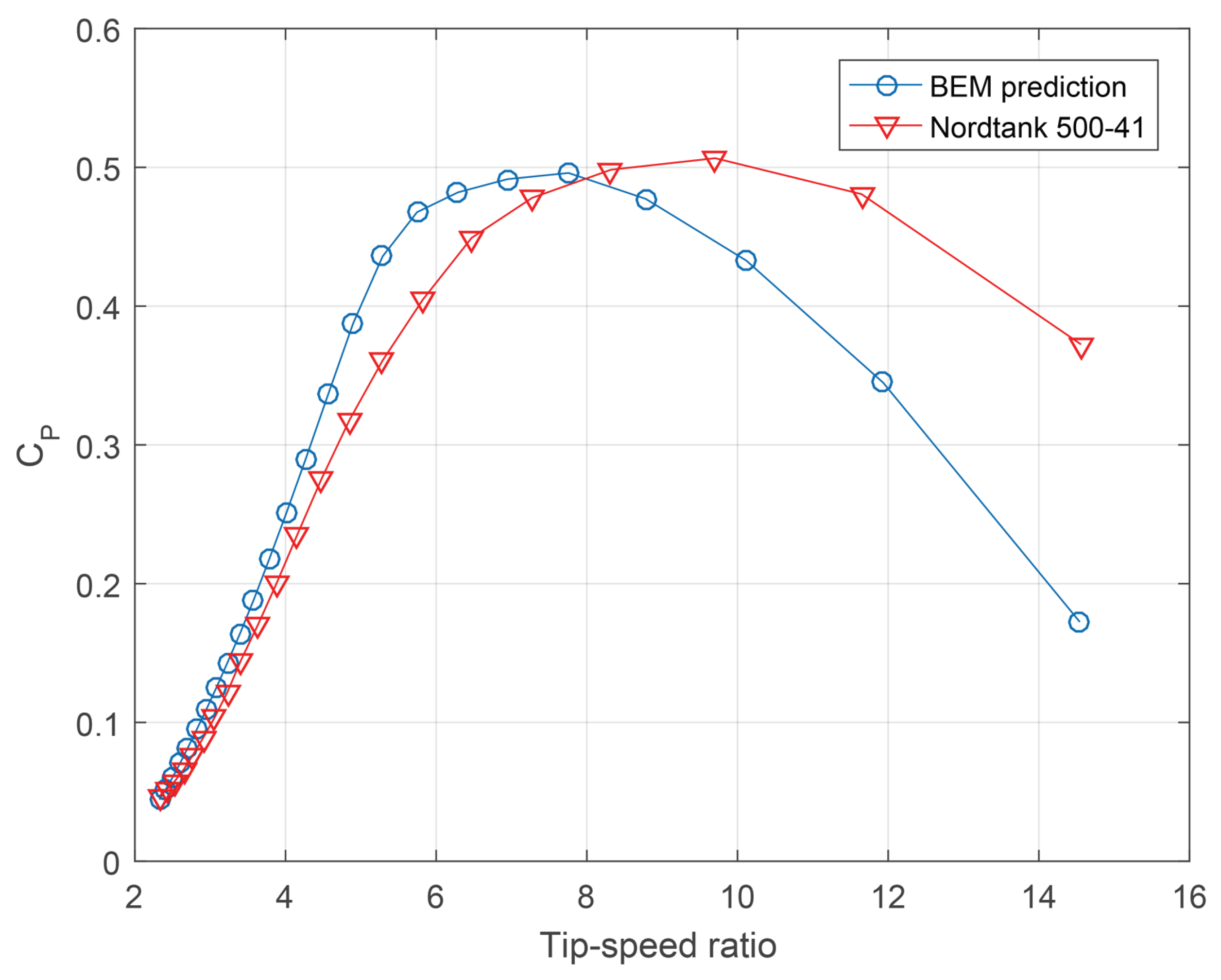
According to the previous specifications, the hypothetical rotor’s blade features a single airfoil along its length; this does not correspond to general practice in wind turbine design but allows for quicker validation of the obtained results. Both the chord and twist distributions are defined based on a similar-sized turbine ([75]). The primary focus of the obtained results is the power coefficient curve C P vs. λ , which can be seen in Figure A1.
Figure A1. BEM result validation and comparison with experimental data ([42]).
Energies 18 05353 g0a1
The final BEM results are compared with the experimental power curve of the Nordtank 500/41 wind turbine, which has a radius of 20.5 m. Its blades are designed with the same airfoil as the one used in the hypothetical turbine over approximately 50% of their length. As shown in Figure A1, the curve corresponding to the implementation of the BEM model is generally similar to the reference case. The power coefficient at low values of λ shows higher results than in the reference case, while, at high λ , C P falls below the reference. The maximum power coefficient, C P , max , is reached at approximately λ = 8 , which is lower than the reference case, where the optimal operating point occurs at a λ close to 10. Finally, it is observed that C P , max does not exceed the reference value or the theoretical Betz limit of approximately 0.593.
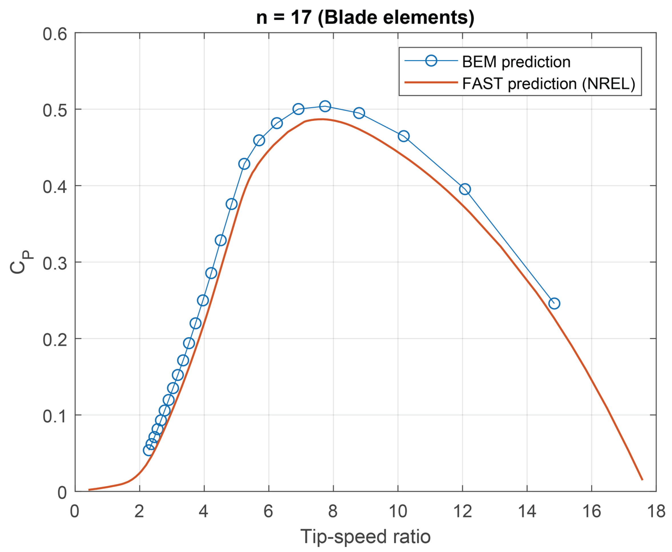
A second validation is carried out with the NREL 5 MW ([75]) wind turbine, which has a diameter of 63 m and uses an NACA 64(3)-615 airfoil in the external radius of the blade and “DU” airfoils in the internal and intermediate radius. The results obtained from this validation are compared with numerical data calculated using the FAST software, as shown in Figure A2. The computed power curve reaches a maximum value of 0.5, compared to 0.48 in the reference data. This difference remains constant across the turbine’s operating range. The overall characteristics of the curve moderately match the reference, as is also the case with the optimal operating point, which is approximately λ = 7.5 .

Appendix A.2. FEM Validation of a Flat Composite Plate with Bend–Twist Coupling

To validate the FEM model’s capability to simulate the laminate’s bend–twist coupling, cross-validation is employed using data acquired from an FEM model of a flat composite plate composed of CFRP, along with experimental data from the literature. The cross-validation method consists of extracting experimental data reported in the literature and comparing it with the data obtained from the developed FEM. Suppose the data from the simulation is close enough to the reported experimental data. In that case, it can be concluded that the developed FEM model yields reliable results and accurately represents the physical phenomenon being studied.
For this particular case, the experimental data reported in the work by Murray et al. [76] were used. In that study, a flat CFRP plate was manufactured to exhibit bend–twist coupling. It was subsequently subjected to an experiment in which cantilever bending was applied, while the rotation angle reached at the tip was measured. The data reported in that work was chosen because of the detailed information on the material’s mechanical properties [76]. The experiment involved the fabrication of a rectangular flat CFRP plate with a stacking sequence of [30/0/30], whose mechanical properties are reported in Table A1. The laminate’s dimensions are 0.5 m in length, 0.2 m in width, and 2.72 mm in thickness. One end of the laminate was clamped, and, at the other end, a point load of 25 N was applied at the center of the width, inducing bending in the laminate.
Figure A2. BEM result validation and numerical data comparison (courtesy of Jason Jonkman, NREL).
Energies 18 05353 g0a2
Table A1. Mechanical properties of the laminate fabricated by Murray et al. used for cross-validation [76].
PropertyValue
E 1 126 GPa
E 2 / E 3 7.7 GPa
ν 12 / ν 23 / ν 31 0.35
G 12 / G 31 3.9 GPa
G 23 2.9 GPa
A numerical FEM simulation of this laminate was programmed in ANSYS APDL and additionally in the laminate design software ESAComp. The latter was used to perform a preliminary design of the laminates for experimental validation, and the obtained data was compared to evaluate its accuracy.
To verify that the FEM results are independent of the number of elements used in the mesh, a mesh independence study was conducted using two different types of elements: a SHELL181 element and a Shell281 element. Various numbers of each of these elements were used, and the resulting maximum displacement ( w m a x ) was compared with the maximum displacement reported in the work of Murray et al. and with the maximum displacement obtained in ESAComp. The results are shown in Table A2 and Figure A3.
According to the mesh independence study, it can be determined that, at the very least, 100 elements must be used to obtain an element-independent result. It can also be determined that results using the shell 181 element obtain the smallest percentage of error; with respect to the angular rotation obtained as a result of the bend–twist coupling on the laminate, in Figure A4, the bending displacement contours experienced by the laminates simulated in ESAComp (left) and ANSYS APDL (right) can be observed, finding that the displacement is greater at one end than at the other along the transverse axis, indicating the presence of rotation in the laminate’s cross-section.
Table A2. Mesh convergence study results for a flat CFRP plate and cross-validation.
ElementNumber of Elements h 2 w m a x (mm)Error (%) (ESAComp)Error (%) (Murray)
SHELL181100.1000124.304.2610.38
1000.0100117.501.285.19
10000.0010118.140.735.71
10,0000.0001118.500.425.99
Shell 281100.1000117.101.624.87
1000.0100118.010.845.60
10000.0010118.460.465.96
10,0000.0001118.500.425.99
w m a x ESAComp (mm) w m a x Murray (mm)
119 111.4
The rotation data at the free end of the laminate were reviewed from the simulation using 100 SHELL181 elements, and a rotation of 10.15° was obtained. Comparing the results with those from Murray et al.’s experiment, the difference is minimal as the reported experimental result was 10.64°, corresponding to a 4.83% error percentage.
The cross-validation results indicate that the use of an FEM model is capable of simulating a bend–twist laminate in the cantilever configuration subjected to a bending load at its free end, obtaining displacement and twist results with an error of approximately 5% compared to the experimental results.
Figure A3. Mesh independence results for cross-validation.
Energies 18 05353 g0a3
Figure A4. FEM simulation results obtained in ESAComp and ANSYS APDL of the laminate reported by Murray et al. [76].
Energies 18 05353 g0a4

Appendix B. Optimal Blade Geometry

Implementing the BEM model enables the calculation of the turbine power coefficient at specified operational conditions as a function of wind and rotational speeds, as well as the blade’s aerodynamic characteristics, such as chord and twist distribution along the blade. Picking up from the torque definition for a differential element of the blade, it is possible to establish a definition for the power associated with each differential element of the blade as a function of both axial and tangential induction factors. Based on the formulation presented by Burton et al. [44]
d P = 4 π ρ ω 2 V a ( 1 a ) r 3 d r .
In this sense, a possible definition for mechanical power can be obtained through the integration of Equation (A1):
P = 4 π ρ ω 2 V 0 R a ( 1 a ) r 3 d r ,
with its dimensionless value corresponding to the power coefficient given by
C P = P 1 2 ρ V 3 A ,
defined as the ratio between the captured mechanical power and the rate of energy of the air stream flowing through the rotor area A; in terms of the induction factors, the power coefficient, C P , is defined as
C P = 8 λ 2 0 λ a ( 1 a ) x 3 d x ,
where λ = ω R / V represents the velocity ratio at the tip of the blade, and x = ω r / V represents the local speed ratio at an arbitrary point along the wingspan of the blade. From the integral expression used for C P , it can be deduced that, for a given rotor size and operating condition, the extracted power can be maximized when the value of the integrand, which is a function of the induction factors, is maximized:
f ( a , a ) = a ( 1 a ) .
On the other hand, the description of the velocity triangle seen in Figure 2 enables establishing a geometric relationship between a and a as follows:
x 2 a ( 1 + a ) = a ( 1 a ) .
To maximize the value of C P , an analytical expression can be formulated taking the derivative of Equation (A5) with respect to a:
f ( a , a ) d a = ( 1 a ) d a d a a = 0 .
When Equation (A6) is derived with respect to a and is combined with Equation (A7), it is possible to find an explicit relationship between a and a :
a = 1 3 a 4 a 1 .
From the established relationships, the axial induction factors that maximize C P depend on the local velocity ratio X; because of this, the optimal a value along the blade is a polynomial defined as
16 a 3 24 a 2 + a ( 9 3 x 2 ) 1 + x 2 = 0 .
Once the optimal distribution is known for both a and a , it is possible to calculate the optimal “twist” angle β opt , which represents the angle between the rotor plane and the local chord section (see Figure 2). This angle can be calculated as
β opt = ϕ α opt ,
where ϕ is calculated as a function of a, a and x = ω r / V . On the other hand, α opt represents the optimal angle of attack defined as a function of the aerodynamic characteristics of the airfoil on each blade element. Chord distribution can be obtained by equalizing the expressions for d T from Equation (3) and the expression from (11), resulting in
c R = 8 π a x s i n 2 ϕ ( 1 a ) B C n λ ,
where the normal force coefficient C n is calculated from (9), taking into account the aerodynamic coefficients at their optimal point, which are C l , opt = C l ( α opt ) and C d , opt = C d ( α opt ) .

Appendix C. Mechanical Testing of Composite Materials

Figure A5. Force and displacement results from material characterization. (a) Tensile–longitudinal; (b) tensile–transverse; (c) compression–longitudinal; (d) compression–transverse; (e) shear–in-plane (12).
Energies 18 05353 g0a5

References

  1. Liao, J.; Liu, X.; Zhou, X.; Tursunova, N.R. Analyzing the role of renewable energy transition and industrialization on ecological sustainability: Can green innovation matter in OECD countries. Renew. Energy 2023, 204, 141–151. [Google Scholar] [CrossRef]
  2. Bashir, M.F.; Pan, Y.; Shahbaz, M.; Ghosh, S. How energy transition and environmental innovation ensure environmental sustainability? Contextual evidence from Top-10 manufacturing countries. Renew. Energy 2023, 204, 697–709. [Google Scholar] [CrossRef]
  3. Liu, W.; Shen, Y.; Razzaq, A. How renewable energy investment, environmental regulations, and financial development derive renewable energy transition: Evidence from G7 countries. Renew. Energy 2023, 206, 1188–1197. [Google Scholar] [CrossRef]
  4. Harichandan, S.; Kar, S.K.; Bansal, R.; Mishra, S.K.; Balathanigaimani, M.S.; Dash, M. Energy transition research: A bibliometric mapping of current findings and direction for future research. Clean. Prod. Lett. 2022, 3, 100026. [Google Scholar] [CrossRef]
  5. Moreno, J.; Cobo, M.; Barraza-Botet, C.; Sanchez, N. Role of low carbon emission H2 in the energy transition of Colombia: Environmental assessment of H2 production pathways for a certification scheme. Energy Convers. Manag. X 2022, 16, 100312. [Google Scholar] [CrossRef]
  6. Torres-Madroñero, J.L.; Nieto-Londoño, C.; Sierra-Pérez, J. Hybrid energy systems sizing for the colombian context: A genetic algorithm and particle swarm optimization approach. Energies 2020, 13, 5648. [Google Scholar] [CrossRef]
  7. Leary, J.; Czyrnek-Delêtre, M.; Alsop, A.; Eales, A.; Marandin, L.; Org, M.; Craig, M.; Ortiz, W.; Casillas, C.; Persson, J.; et al. Finding the niche: A review of market assessment methodologies for rural electrification with small scale wind power. Renew. Sustain. Energy Rev. 2020, 133, 110240. [Google Scholar] [CrossRef]
  8. Bianchini, A.; Bangga, G.; Baring-Gould, I.; Croce, A.; Cruz, J.I.; Damiani, R.; Erfort, G.; Simao Ferreira, C.; Infield, D.; Nayeri, C.N.; et al. Current status and grand challenges for small wind turbine technology. Wind Energy Sci. 2022, 7, 2003–2037. [Google Scholar] [CrossRef]
  9. López-Castrillón, W.; Sepúlveda, H.H.; Mattar, C. Off-grid hybrid electrical generation systems in remote communities: Trends and characteristics in sustainability solutions. Sustainability 2021, 13, 5856. [Google Scholar] [CrossRef]
  10. Pourrajabian, A.; Rahgozar, S.; Dehghan, M.; Wood, D. A comprehensive multi-objective optimization study for the aerodynamic noise mitigation of a small wind turbine. Eng. Anal. Bound. Elem. 2023, 155, 553–564. [Google Scholar] [CrossRef]
  11. Battisti, L.; Benini, E.; Brighenti, A.; Dell’Anna, S.; Raciti Castelli, M. Small wind turbine effectiveness in the urban environment. Renew. Energy 2018, 129, 102–113. [Google Scholar] [CrossRef]
  12. Cruz Cruz, I.; Toja, F.; Cano, L.; Arribas, L.; Hsu, C.C.; Tinnesand, H.; Kelley, N. IEA Wind TCP Task 27 Small Wind Turbine Technical Report; Technical Report; IEA Wind Technology Collaboration Programme: Copenhagen, Denmark, 2018. [Google Scholar]
  13. Singh, R.K.; Ahmed, M.R.; Zullah, M.A.; Lee, Y.H. Design of a low Reynolds number airfoil for small horizontal axis wind turbines. Renew. Energy 2012, 42, 66–76. [Google Scholar] [CrossRef]
  14. Papi, F.; Pagamonci, L.; Bianchini, A. Design Loads in Small Wind Turbines: A Detailed Comparison between Pitch and Stall Regulation. J. Phys. Conf. Ser. 2022, 2385, 012120. [Google Scholar] [CrossRef]
  15. Gawad, A.F. Novel electro-mechanical mechanism for blade pitch-control of horizontal-axis, home-scale wind turbines. In Proceedings of the 10th Annual International Energy Conversion Engineering Conference, IECEC 2012, Atlanta, GA, USA, 30 July–1 August 2012. [Google Scholar] [CrossRef]
  16. Wang, P.; Bao, D.; Zhao, M.; Shi, Z.; Gao, F.; Han, F. The Design, Analysis, and Optimization of a New Pitch Mechanism for Small Wind Turbines. Energies 2023, 16, 6708. [Google Scholar] [CrossRef]
  17. Elkodama, A.; Ismaiel, A.; Abdellatif, A.; Shaaban, S.; Yoshida, S.; Rushdi, M.A. Control Methods for Horizontal Axis Wind Turbines (HAWT): State-of-the-Art Review. Energies 2023, 16, 6394. [Google Scholar] [CrossRef]
  18. Torres-Madroñero, J.L.; Alvarez-Montoya, J.; Restrepo-Montoya, D.; Tamayo-Avendaño, J.M.; Nieto-Londoño, C.; Sierra-Pérez, J. Technological and operational aspects that limit small wind turbines performance. Energies 2020, 13, 6123. [Google Scholar] [CrossRef]
  19. Vilà, J.; Luo, N.; Pacheco, L.; Pujol, T.; Gonzalez, J.R.; Ferrer, I.; Massaguer, A.; Massaguer, E. Design of an active pitch control for small horizontal-axis wind turbine. Renew. Energy Power Qual. J. 2021, 19, 195–198. [Google Scholar] [CrossRef]
  20. Maheri, A.; Noroozi, S.; Toomer, C.; Vinney, J. A simple algorithm to modify an ordinary wind turbine blade to an adaptive one. In Proceedings of the European Wind Energy Conference, Athens, Greece, 27 February–2 March 2006; Volume 2, pp. 1195–1202. [Google Scholar]
  21. Nicholls-Lee, R.F.; Turnock, S.R. Enhancing performance of a horizontal axis tidal turbine using adaptive blades. In Proceedings of the OCEANS 2007—Europe, Aberdeen, UK, 18–21 June 2007. [Google Scholar] [CrossRef]
  22. Barr, S.M.; Jaworski, J.W. Optimization of tow-steered composite wind turbine blades for static aeroelastic performance. Renew. Energy 2019, 139, 859–872. [Google Scholar] [CrossRef]
  23. Capuzzi, M.; Pirrera, A.; Weaver, P.M. Structural design of a novel aeroelastically tailored wind turbine blade. Thin-Walled Struct. 2015, 95, 7–15. [Google Scholar] [CrossRef]
  24. Capuzzi, M.; Pirrera, A.; Weaver, P.M. A novel adaptive blade concept for large-scale wind turbines. Part I: Aeroelastic behaviour. Energy 2014, 73, 15–24. [Google Scholar] [CrossRef]
  25. Capuzzi, M.; Pirrera, A.; Weaver, P.M. A novel adaptive blade concept for large-scale wind turbines. Part II: Structural design and power performance. Energy 2014, 73, 25–32. [Google Scholar] [CrossRef]
  26. Tamayo-Avendaño, J.M.; Patiño-Arcila, I.D.; Nieto-Londoño, C.; Sierra-Pérez, J. Fluid–Structure Interaction Analysis of a Wind Turbine Blade with Passive Control by Bend–Twist Coupling. Energies 2023, 16, 6619. [Google Scholar] [CrossRef]
  27. Sun, W.; Li, Y.; Shi, Q.; Ouyang, T.; Ma, L. Passive aeroelastic study of large and flexible wind turbine blades for load reduction. Structures 2023, 58, 105331. [Google Scholar] [CrossRef]
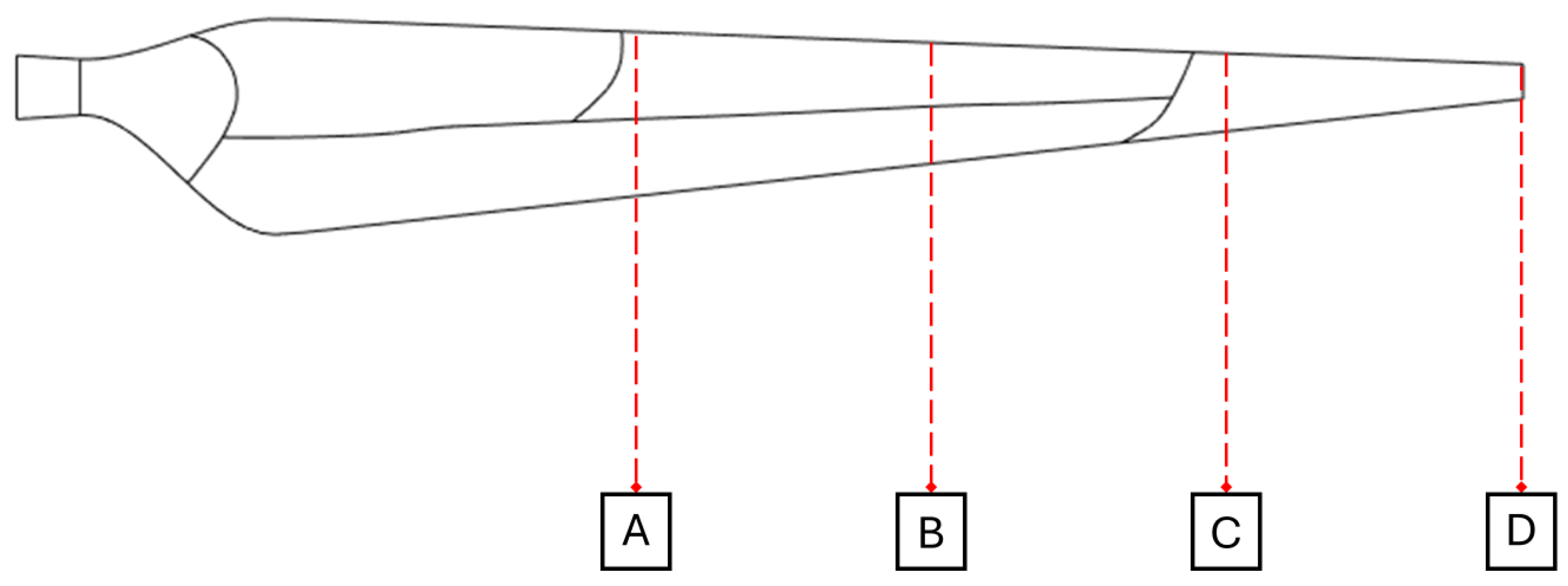
  28. Papadakis, N.; Condaxakis, C. An Experimental Performance Assessment of a Passively Controlled Wind Turbine Blade Concept: Part A—Isotropic Materials. Energies 2024, 17, 3049. [Google Scholar] [CrossRef]
  29. Papadakis, N.; Condaxakis, C. An Experimental Performance Assessment of a Passively Controlled Wind Turbine Blade Concept: Part B—Material Oriented with Glass-Fiber-Reinforced Polymer. Energies 2024, 17, 3286. [Google Scholar] [CrossRef]
  30. Farias, T.; Tavares da Silva, C.; Luersen, M. A Surrogate-Based Approach for Bend-Twist Coupling Optimization of a Horizontal Axis Wind Turbine Composite Blade. In Proceedings of the Ibero-Latin American Congress on Computational Methods in Engineering (CILAMCE), Maceió, Brazil, 11–14 November 2024. [Google Scholar] [CrossRef]
  31. Restrepo-Montoya, D.; Alvarez-Montoya, J.; Sierra-Pérez, J.; Nieto-Londoño, C. Artificial Intelligence Metamodeling Approach to Design Smart Composite Laminates with Bend-Twist Coupling. In Proceedings of the 2019 IEEE 2nd International Conference on Renewable Energy and Power Engineering (REPE), Toronto, ON, Canada, 2–4 November 2019; pp. 155–159. [Google Scholar]
  32. Herath, M.T.; Lee, A.K.L.; Prusty, B.G. Design of shape-adaptive wind turbine blades using Differential Stiffness Bend-Twist coupling. Ocean Eng. 2015, 95, 157–165. [Google Scholar] [CrossRef]
  33. Maheri, A.; Noroozi, S.; Vinney, J. Application of combined analytical/FEA coupled aero-structure simulation in design of wind turbine adaptive blades. Renew. Energy 2007, 32, 2011–2018. [Google Scholar] [CrossRef]
  34. Vesel, R.W.; McNamara, J.J. Performance enhancement and load reduction of a 5MW wind turbine blade. Renew. Energy 2014, 66, 391–401. [Google Scholar] [CrossRef]
  35. Scott, S.; Capuzzi, M.; Langston, D.; Bossanyi, E.; McCann, G.; Weaver, P.M.; Pirrera, A. Effects of aeroelastic tailoring on performance characteristics of wind turbine systems. Renew. Energy 2017, 114, 887–903. [Google Scholar] [CrossRef]
  36. Babuska, P.; Wiebe, R.; Motley, M.R. A beam finite element for analysis of composite beams with the inclusion of bend-twist coupling. Compos. Struct. 2018, 189, 707–717. [Google Scholar] [CrossRef]
  37. Hayat, K.; Ha, S.K. Load mitigation of wind turbine blade by aeroelastic tailoring via unbalanced laminates composites. Compos. Struct. 2015, 128, 122–133. [Google Scholar] [CrossRef]
  38. Zahle, F.; Tibaldi, C.; Pavese, C.; McWilliam, M.K.; Blasques, J.; Hansen, M.H. Design of an Aeroelastically Tailored 10 MW Wind Turbine Rotor. J. Phys. Conf. Ser. 2016, 753, 062008. [Google Scholar] [CrossRef]
  39. Manolas, D.I.; Serafeim, G.P.; Chaviaropoulos, P.K.; Riziotis, V.A.; Voutsinas, S.G. Assessment of load reduction capabilities using passive and active control methods on a 10 MW-scale wind turbine. J. Phys. Conf. Ser. 2018, 1037, 032042. [Google Scholar] [CrossRef]
  40. Tamayo-Avendaño, J. Design of an Aeroelastic Passive Control Strategy for a Fixed-Pitch Horizontal-Axis Wind Turbine. Ph.D. Thesis, Universidad Pontificia Bolivariana, Medellín, Colombia, 2023. [Google Scholar]
  41. Saverin, J.; Peukert, J.; Marten, D.; Pechlivanoglou, G.; Paschereit, C.O.; Greenblatt, D. Aeroelastic simulation of multi-MW wind turbines using a free vortex model coupled to a geometrically exact beam model. J. Phys. Conf. Ser. 2016, 753, 082015. [Google Scholar] [CrossRef]
  42. Hansen, M.O. Aerodynamics of Wind Turbines; Earthscan: Oxfordshire, UK, 2008; Volume 17. [Google Scholar]
  43. Hansen, M.O.L.; Sørensen, J.N.; Voutsinas, S.; Sørensen, N.; Madsen, H.A. State of the art in wind turbine aerodynamics and aeroelasticity. Prog. Aerosp. Sci. 2006, 42, 285–330. [Google Scholar] [CrossRef]
  44. Burton, T.; Sharpe, D.; Jenkins, N.; Bossanyi, E. Wind Energy Handbook, 1st ed.; Wiley: Hoboken, NJ, USA, 2001. [Google Scholar]
  45. Pawlowski, L.; Dudzinska, M.R.; Pawlowski, A. Environmental Science and Engineering: Environmental Engineering; Springer: Berlin/Heidelberg, Germany, 2013. [Google Scholar]
  46. Giguère, P.; Selig, M.S. New airfoils for small horizontal axis wind turbines. J. Sol. Energy Eng. Trans. ASME 1998, 120, 108–114. [Google Scholar] [CrossRef]
  47. Tangler, J.L.; Somers, D.M. NREL Airfoil Families for HAWTs; Technical Report; National Renewable Energy Laboratory: Golden, CO, USA, 1995.
  48. Somers, D.M. The S822 and S823 Airfoils; Technical Report; National Renewable Energy Laboratory: Golden, CO, USA, 2005.
  49. Lyon, C.A.; Broeren, A.P.; Guigère, P.; Gopalarathnam, A.; Selig, M.S. Summary of Low-Speed Airfoil Data; SoarTech Publications: Virginia Beach, VA, USA, 1997; Volume 3. [Google Scholar]
  50. ASTM D3039/D3039M-17; Test Method for Tensile Properties of Polymer Matrix Composite Materials. ASTM: West Conshohocken, PA, USA, 2017. [CrossRef]
  51. ASTM D638-22; Standard Test Method for Tensile Properties of Plastics. ASTM: West Conshohocken, PA, USA, 2022. [CrossRef]
  52. ASTM D695-15; Test Method for Compressive Properties of Rigid Plastics. ASTM: West Conshohocken, PA, USA, 2015. [CrossRef]
  53. ASTM D5379/D5379M-19; Test Method for Shear Properties of Composite Materials by the V-Notched Beam Method. ASTM: West Conshohocken, PA, USA, 2019. [CrossRef]
  54. Jones, R.M. Mechanics of Composite Materials, 2nd ed.; Taylor & Francis, Inc.: Abingdon, UK, 1998. [Google Scholar]
  55. Michalewicz, Z. Genetic Algorithms + Data Structures = Evolution Programs; Springer: Berlin/Heidelberg, Germany, 1992. [Google Scholar]
  56. ANSYS, Inc. Ansys® Mechanical APDL Theory Reference, Release 2021 R2; ANSYS: Canonsburg, PA, USA, 2021. [Google Scholar]
  57. Newmark, N.M. A method of computation for structural dynamics. J. Eng. Mech. Div. 1959, 85, 67–94. [Google Scholar] [CrossRef]
  58. Hilber, H.M.; Hughes, T.J.R.; Taylor, R.L. Improved numerical dissipation for time integration algorithms in structural dynamics. Earthq. Eng. Struct. Dyn. 1977, 5, 283–292. [Google Scholar] [CrossRef]
  59. Liu, G.; Quek, S. The Finite Element Method: A Practical Course; Butterworth-Heinemann: Oxford, UK, 2003. [Google Scholar]
  60. Mindlin, R. Influence of rotatory inertia and shear on flexural motions of isotropic elastic plates. Appl. Mech. 1951, 18, 31–38. [Google Scholar] [CrossRef]
  61. Reissner, E. The effect of transverse shear deformation on the bending of elastic plates. Am. Soc. Mech. Eng. 1945, 12, A68–A77. [Google Scholar] [CrossRef]
  62. Camp, C.; Pezeshk, S.; Cao, G. Optimized design of two-dimensional structures using a genetic algorithm. J. Struct. Eng. 1998, 124, 551–559. [Google Scholar] [CrossRef]
  63. Delyová, I.; Frankovskỳ, P.; Bocko, J.; Trebuňa, P.; Živčák, J.; Schürger, B.; Janigová, S. Sizing and topology optimization of trusses using genetic algorithm. Materials 2021, 14, 715. [Google Scholar] [CrossRef]
  64. Jebari, K. Parent Selection Operators for Genetic Algorithms. Int. J. Eng. Res. Technol. 2013, 12, 1141–1145. [Google Scholar]
  65. Mehboob, U.; Qadir, J.; Ali, S.; Vasilakos, A. Genetic algorithms in wireless networking: Techniques, applications, and issues. Soft Comput. 2016, 20, 2467–2501. [Google Scholar] [CrossRef]
  66. Sberna, A.P.; Demartino, C.; Vanzi, I.; Marano, G.C.; Di Trapani, F. Cost-effective topology optimization of masonry structure reinforcements by a linear static analysis-based GA framework. Bull. Earthq. Eng. 2024, 22, 4143–4167. [Google Scholar] [CrossRef]
  67. Zhang, W.; Zhao, Y.; Wu, Z.; Zhao, J.; Wang, S. The Application of Genetic Algorithm in Seismic Performance Optimization of a Y-Eccentrically Braced Composite Frame. Buildings 2025, 15, 770. [Google Scholar] [CrossRef]
  68. Hand, M.M.; Simms, D.A.; Fingersh, L.J.; Jager, D.W.; Cotrell, J.R.; Schreck, S.; Larwood, S.M. Unsteady Aerodynamics Experiment Phase VI: Wind Tunnel Test Configurations and Available Data Campaigns; National Renewable Energy Laboratory (NREL): Golden, CO, USA, 2001.
  69. Sørensen, N.N.; Michelsen, J.A.; Schreck, S. Navier–Stokes predictions of the NREL phase VI rotor in the NASA Ames 80 ft × 120 ft wind tunnel. Wind Energy 2002, 5, 151–169. [Google Scholar] [CrossRef]
  70. Lee, K.; Huque, Z.; Kommalapati, R.; Han, S.E. Fluid-structure interaction analysis of NREL phase VI wind turbine: Aerodynamic force evaluation and structural analysis using FSI analysis. Renew. Energy 2017, 113, 512–531. [Google Scholar] [CrossRef]
  71. Wu, W.; Wang, Q.; Li, W. Comparison of Tensile and Compressive Properties of Carbon/Glass Interlayer and Intralayer Hybrid Composites. Materials 2018, 11, 1105. [Google Scholar] [CrossRef]
  72. Burgani, T.d.S.; Alaie, S.; Tehrani, M. Modeling Flexural Failure in Carbon-Fiber-Reinforced Polymer Composites. J. Compos. Sci. 2022, 6, 33. [Google Scholar] [CrossRef]
  73. Ozyildiz, M.; Muyan, C.; Coker, D. Strength Analysis of a Composite Turbine Blade Using Tsai–Wu and Puck Failure Criteria. J. Phys. Conf. Ser. 2018, 1037, 042027. [Google Scholar] [CrossRef]
  74. Staino, A.; Basu, B. Emerging trends in vibration control of wind turbines: A focus on a dual control strategy. Philos. Trans. R. Soc. A Math. Phys. Eng. Sci. 2015, 373, 20140069. [Google Scholar] [CrossRef] [PubMed]
  75. Jonkman, J.; Butterfield, S.; Musial, W.; Scott, G. Definition of a 5-MW Reference Wind Turbine for Offshore System Development; Technical Report; National Renewable Energy Laboratory (NREL): Golden, CO, USA, 2009.
  76. Murray, R.E.; Doman, D.A.; Pegg, M.J. Finite element modeling and effects of material uncertainties in a composite laminate with bend–twist coupling. Compos. Struct. 2015, 121, 362–376. [Google Scholar] [CrossRef]
Figure 1. Methodology flowchart for blade design.
Energies 18 05353 g001
Figure 2. Velocity triangle shown in a cross-section of the rotor blade.
Energies 18 05353 g002
Figure 3. Flowchart of the BEM model showing initialization and postprocessing steps (green rounded rectangles), iterative computations (blue rectangles), and the convergence check (yellow diamond).
Energies 18 05353 g003
Figure 4. S822 polars calculated at R e = 300,000 ([47,48]).
Energies 18 05353 g004
Figure 5. SG6043 polars calculated at R e = 300,000 ([46,49]).
Energies 18 05353 g005
Figure 6. Tensile test specimens. (a) Before the test; (b) after the test.Test specimen numbers correspond to the results presented in Figure A5.
Energies 18 05353 g006
Figure 7. Compressive test specimens. (a) Before the test; (b) after the test. Test specimen numbers correspond to the results presented in Figure A5.
Energies 18 05353 g007
Figure 8. Genetic algorithm flowchart. Initialization and final steps (green rounded rectangles), computational processes in MATLAB (blue rectangles), objective function evaluation in ANSYS APDL (yellow rectangle), and convergence decision (diamond).
Energies 18 05353 g008
Figure 9. Fluid flow domain and boundary layout. A: velocity inlet; B: slip walls; C: periodic boundaries for sliding mesh; D: no-slip wall; E: periodic boundaries; F: pressure outlet Tamayo-Avendaño et al. [26].
Energies 18 05353 g009
Figure 10. Fluid flow domain and mesh details. (a) General mesh layout; (b) boundary layer inflation. Colors in figure (a) represent different volumes used to define the mesh as presented in Figure 9.
Energies 18 05353 g010
Figure 11. Blade domain for structural assessment. (a) Laminate thickness; (b) finite element mesh.
Energies 18 05353 g011
Figure 12. Blade ideal geometry at operating point.
Energies 18 05353 g012
Figure 13. Entire blade design details.
Energies 18 05353 g013
Figure 14. Principal material directions in a unidirectional fiber-reinforced composite. (a) Isometric view of the fiber orientation; (b) Transversal and longitudinal plane view.
Energies 18 05353 g014
Figure 15. Laminate design. (a) Stacking sequence; (b) view of the division by structural region and fiber orientation.
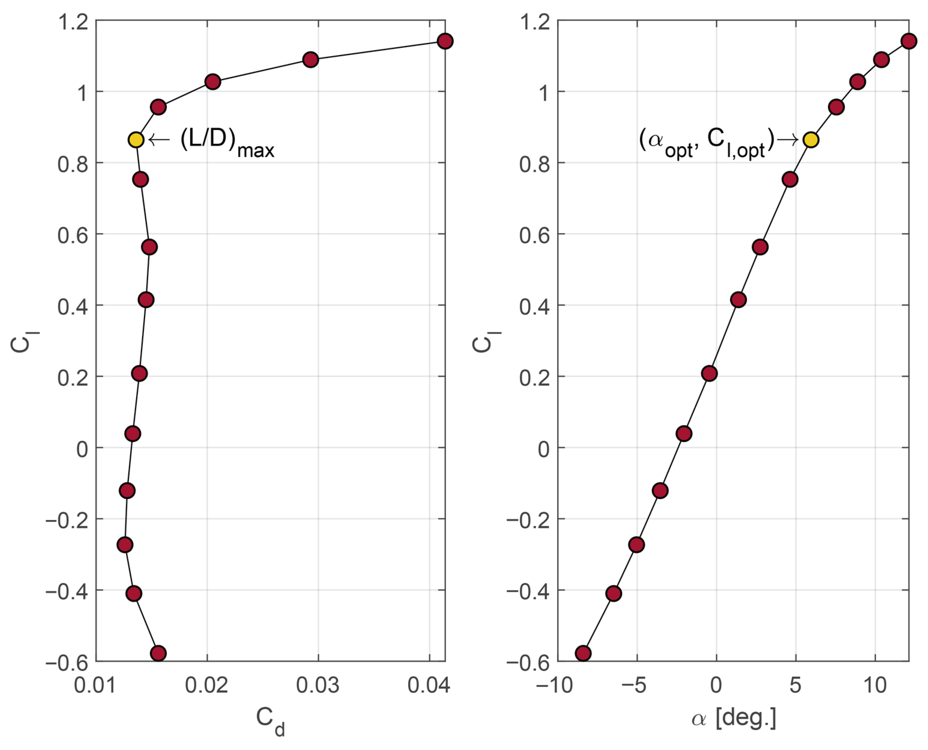
Energies 18 05353 g015
Figure 16. Tsai–Wu failure analysis on blade.
Energies 18 05353 g016
Figure 17. Pressure contour results for cut-in operation at wind speed of 2 m/s.
Energies 18 05353 g017
Figure 18. Lift and drag aerodynamic coefficient results from CFD simulation. (a) Cut-in C L ; (b) cut-in C D ; (c) operation 1 C L ; (d) operation 1 C D ; (e) operation 2 C L ; (f) operation 2 C D ; (g) operation 3 C L ; (h) operation 3 C D ; (i) cut-out C L ; (j) cut-out C D .
Energies 18 05353 g018
Figure 19. Change in the blade twist due to aerodynamic force.
Energies 18 05353 g019
Figure 20. α l variation due to structural bend–twist coupling in different sections of the blade. (a) Monitor A; (b) monitor B; (c) monitor C; (d) monitor D.
Energies 18 05353 g020
Figure 21. Monitor locations for α l variation. Marks A, B, C, and D correspond to the blade section monitors shown in the Figure 20.
Energies 18 05353 g021
Figure 22. BEM results of angle of attack.
Energies 18 05353 g022
Figure 23. BEM results of aerodynamic coefficient. (a) Lift coefficient; (b) drag coefficient.
Energies 18 05353 g023
Figure 24. BEM results of loads on blade. (a) Normal load; (b) tangential load.
Energies 18 05353 g024
Figure 25. BEM results as a function of wind speed. (a) Power generation; (b) power coefficient.
Energies 18 05353 g025
Figure 26. BEM results of structural loads as a function of wind speed. (a) Thrust; (b) torque.
Energies 18 05353 g026
Table 1. Average maximum load and maximum stress obtained from tensile, compressive, and shear tests along principal directions.
Test Type and Direction F max [N] σ max [GPa]
Tensile–Longitudinal59,471.801.98
Tensile–Transverse1161.660.022
Compression–Longitudinal6880.030.26
Compression–Transverse2412.670.11
Shear–In-plane (12)1729.360.075
Table 2. Average elastic properties obtained from tensile and compression tests of the carbon fiber composite.
PropertyTensile TestCompression Test
E 1 [GPa]26.0828.22
E 2 [GPa]6.269.12
E 3 [GPa]6.269.12
ν 23 0.3700.311
ν 12 0.3370.340
ν 13 0.3370.340
Table 3. Average in-plane ( G 12 ) and out-of-plane ( G 23 ) shear moduli of the carbon fiber composite obtained from mechanical testing.
PropertyValue
G 12 [GPa]1.44
G 31 [GPa]1.44
G 23 [GPa]1.18
Table 4. Laminate layup sequence.
Ply GroupPly CountLaminate Sequence
Tip2[ 72 / 72 ]
Mid 34[ 2 / 60 / 60 / 2 ]
Mid 22[ 2 / 2 ]
Mid 14[ 68 / 72 / 72 / 68 ]
Root8[ 4 / 62 / 84 / 78 / 78 / 84 / 62 / 4 ]
Table 5. Simulation cases evaluated.
Simulation Case V  [m/s] ω  [rpm] θ  [deg]
Cut-in2/2.5/30 9
Opr-19/10/112500
Opr-214/15/162500
Opr-319/20/212500
Cut-out26/28/302500
Disclaimer/Publisher’s Note: The statements, opinions and data contained in all publications are solely those of the individual author(s) and contributor(s) and not of MDPI and/or the editor(s). MDPI and/or the editor(s) disclaim responsibility for any injury to people or property resulting from any ideas, methods, instructions or products referred to in the content.