Article

Versatile LCL Inverter Model for Controlled Inverter Operation in Transient Grid Calculation Using the Extended Node Method

Chair of Electrical Power Systems, Helmut Schmidt University/University of the Federal Armed Forces Hamburg, Holstenhofweg 85, D-22043 Hamburg, Germany
*
Author to whom correspondence should be addressed.
Energies 2025, 18(2), 344; https://doi.org/10.3390/en18020344
Submission received: 30 November 2024 / Revised: 5 January 2025 / Accepted: 8 January 2025 / Published: 14 January 2025

Abstract

:
Due to increasing decentralized power applications, power electronics are gaining importance, also in distribution grids. Since their scope of investigation is diverse, their versatile models and their use in grid calculations are important. In this work, a three-phase grid-synchronous inverter with an LCL filter is considered. It is defined as a component of the “Extended Node Method” to make it applicable in this node-based transient grid calculation method. Because the component stucture always looks the same and the construction of the grid system of equations always follows the same, straightforward process, the model can be applied easily and several times to large network calculations. Furthermore, an approach is developed for how inverter control algorithms are interconnected with the method’s results in the time domain. This allows for the fast analysis of converter control schemes in different grid topologies. To evaluate its accuracy, the developed approach is compared to equivalent calculations with Simulink and shows very good agreement, also for steep transients. In the long term, this model is intended to bridge the gap to other DC systems like electrochemical components and to gas and heating networks with the Extended Node Method.

1. Introduction

The use of power electronics is becoming increasingly important for future decentralized generation, also including DC appliances such as photovoltaics or batteries. Since these power electronics have different dynamic behavior than conventional generators, and also can be small and distributed, there are many challenges in the context of the transition from traditional energy supply to more decentralized energy supply in the AC power grid. Although a complete abandonment of powerful central power plants and their reserve capacities and, hence, a finalized decentralization of power generation are currently not yet possible for economic reasons and due to the complexity of managing multiple plants and their maintenance, decentralization offers some advantages. The power transport losses decrease and also a smaller dimensioning of the required transmission capacity of main power transmission lines becomes possible. In addition, the impact of faults in central power plants or main power transmission lines is reduced. Power electronics are also indispensable when it comes to connecting electrochemical components to the grid: electrolyzers, in particular, can convert excess renewable electrical power into storable gas, while heat-controlled fuel cells require a joint consideration with local heating supply. Therefore, considering power electronics is necessary when it comes to cross-energy management strategies and network analysis, and of integrated power, gas, and heating grids.
Researchers are tackling these numerous challenges in terms of power electronics in various subject areas, such as filter design, inverter control, and stability analyses. The main subject of this work is a three-phase inverter with an LCL filter. Due to its design, a high impedance for high-frequency components can be achieved, whereas few losses occur at the fundamental grid frequency. But they have a resonance point whose position and deflection must be taken into account when designing the passive filter components to guarantee safe and stable inverter operation [1]. Since in most cases not all the characteristics of the grid to which an inverter is to be connected are known, the design should be as robust as possible. Hence, there is a lot of research in the field of filter design [1,2,3,4,5,6]. The improved robust approach in [2] can be used in a wide range of grid impedance. The authors in [3] also provide guide values and limits for inductors and capacitors’ in particular, they show how passive damping affects the frequency behavior of the filter. In [7,8], the authors analyze the power injection capability of inverters as a function of grid impedance and the short-cut ratio between the grid and inverter. The general modeling of single inverters is part of [9,10,11]. In addition to the model explanations, Ref. [9] also provides detailed insight on the control of voltage source converters. In [12], a review on single converter models is provided. Suitable model types are described based on relevant stability issues. In [13], the authors give an overview on power system modeling with inverter-interfaced generation and in [14], the focus is on the formulation of steady-state power-flow in inverter-based grids. The development of control strategies is also a large field when it comes to inverters with an LCL filter. Since there are many different purposes and fields of applications for inverter control, research in this area is correspondingly diverse: In [15,16,17], some guidelines for inverter controller designs are given. In [18], a current control is proposed for the inverter-side current. The authors in [19] especially challenge the problem of inverter-side current control, which is weak in suppressing harmonics in the grid current under a distorted grid state; also, ref. [20] gives an approach for grid current control. In [21,22], cascaded control schemes are presented to divide the LCL three order system into three one-order systems. In [23], control and stability analysis for LCL grid-connected converters is performed, especially addressing the challenge of phase-locked-loop (PLL) and current control coupling for weak grid conditions. In [24], a robust control scheme which works under grid disturbances is presented. The authors in [25] developed an improved control strategy for inverters with LCL filters which uses a novel reduced-order observer so that only one sensor is needed. The authors in [26] address the LCL filter design, as well as strategies for resonance damping: in addition to passive damping strategies, active damping approaches by capacitor current or voltage feedback or by inserting a notch transfer function are also presented and investigated. In [27], a parallel feedforward compensation design which achieves efficient damping, good control characteristics, and better robustness in terms of filter paremeter variations is explored. In recent research, e.g., [28,29,30,31], approaches using artificial intelligence (AI) can be found in the field of inverters and inverter-based grids. The review in [28] provides an overview of AI-based controllers and discusses the benefits. The work in [29] presents an approach for AI-based single-phase converter control and the work in [30] discusses a three-phase neutral back-to-back power converter for wind energy conversion. The authors in [31] use AI for diagnosis and fault detection for grid-connected photovoltaic systems. Since the investigation of inverter behavior is important and cannot be limited to only considering one inverter, tools are necessary that allow the simultaneous observation of several inverters and can show their effects on the grid, including critical transients. Therefore, simple and universally applicable models of inverters that work well with transient network calculations are useful. The authors in [32] address this field by developing an inverter model for the electrical engineering software PLECS [33]. Also, other established software tools such as DIgSILENT PowerFactory [34] and Simulink [35] offer models for power electronic components. Whereas Simulink makes it difficult to set up very large network structures, Powerfactory in particular is very well suited for network calculations in large grid topologies, including electromagnetic transients, asymmetrical network conditions, and fault events. The work presented here also makes its contribution to dynamic inverter modeling for large grid calculations. It contains the modeling of a controlled inverter component with an LCL filter as a universally applicable component in the “Extended Node Method”. This method is used for the transient calculation of electrical power grids based only on node equations [36,37]. For this purpose, components and nodes are classified as special types, which leads to an Differential-Algebraic-Equation-System (DAE). This method was also addressed and used in [38,39,40,41,42,43,44,45]. Although the work in [36] gives detailed explanations on the characterization of conventional AC components for the ENM, it is lacking when it comes to power electronics. Therefore, an inverter with an LCL filter is now made available for this method as an example of a power electronic converter within this work. In addition, a design interface of the method-specific DAE in ‘abc’ and a subordinate inverter control scheme in ‘dq’ are developed. This means that prospectively any type of control for LCL filters can be easily included into the ENM. This makes this work a tool that is easy to use for research in the field of controller design. Since the inverter model always has the same structure due to its characterization, large grid calculations with one or more controlled inverters are possible with the ENM. Thus, a framework for testing control strategies in combination with transient grid calculations is provided here. Based on this, many studies on stability can be carried out, since the grid does not have to be rigid and interactions between different active network components are considered. However, since the ENM can also simulate grid faults easily using the fault matrix method [36], the behavior of inverters in the event of fault can also be investigated. But further use of the model is not limited to the AC side: one can also take a look at the other side of the inverter, since it enables a path to DC applications like electrochemical components [46,47] to be calculated together with the ENM. In contrast to PLECS and Digsilent Powerfactory, this method is not limited to electrical aspects but can be further developed for combined cross-energy grid calculations regarding electric power, gas, and heating grids [48].
This paper is structured as follows: In Section 2, firstly, the basic principle of the ENM is explained in terms of the method-specific component and node definitions and the structure of the DAE are given in Section 2.1. In Section 2.2, a three-phase grid-tied inverter with an LCL filter is considered and special requirements of the filter design are briefly discussed. In Section 2.3, the inverter with the LCL filter is embedded into the ENM. Based on its electric circuit diagram, the parameters for the component matrices are derived. Also, it is stated where the variables occur in the DAE. Subsequently, a cascaded control system for grid-following inverters with an LCL filter is then proposed as an example for inverter control. In Section 2.5, the developed general software tool including the ENM with embedded inverters is briefly described and a visualization of the combined control and grid calculation algorithm is presented. To validate the accuracy of the method, results for transient network calculations with controlled inverters are compared with Simulink/Simscape R2024b in Section 3. In Section 4, the main achievements of the presented work are summarized and an outlook on the further application of the inverter component and the further extension of the ENM is given.

2. Materials and Methods

In the following, the used and derived materials and methods are described. Firstly, the ENM and its characteristic classification of components and nodes are presented. In Section 2.2, the general model of the two-level three-phase inverter with an LCL filter is taken up and the relevant criteria for designing the filter parameters are briefly introduced. Subsequently, the LCL inverter is embedded into the ENM in Section 2.3, whereby a distinction is made between the basic model and circuits with damping resistors. Also, the sensitivity of the filter parameters and how they affect the system of equations are also briefly addressed. In Section 2.4, an inverter control algorithm is introduced, which will be used in this work to operate the grid-connected LCL inverters. The structure of the software tool and the methodology for the combined inverter control and grid calculation algorithm with the ENM are presented in Section 2.5.

2.1. The Extended Node Method

The ENM is a method for transient electric grid calculation [36,37]. One major advantage is that it is based only on nodal equations and therefore the elaborate formulation of mesh equations can be omitted [36]. To obtain these nodal equations, all grid components are classified according to their terminal behavior concerning voltage u and current i. The three main types are the following: L components with inductive behavior, R components with resistive behavior, and C components with capacitive behavior. One-port components are of type ‘A’, whereas two-ports are named ‘AB’ components. The general explicit state equations for the different component types are listed in Table 1.
The individual component parameters are collected in component matrices in diagonal form, preferably sorted according to A and AB components. The resistors  R L  of L components are part of  R L  and their inductive conductances  G L = 1 ω 0 L  are part of  G L  and  G L , diag . G L , diag .  only differs from  G L  for L-AB components without an inner cross-branch (cf. Section 8.8.2 in [36]). Resisitive conductance values of R components  G R = 1 R  are consolidated in  G R . For C components, their capacitances are sorted in  C C  and parallel conductances in  G C . Source voltages ( u scL ) or source currents ( i scR i scC ) can also occur in components.
Also, the nodes are divided into three different groups in the ENM: L, R, and C nodes. The node classification depends on the connected components according to the following scheme (cf. [36]):
n o d e   t y p e = L   n o d e L   c o m p o n e n t s   m a n d a t o r y R   n o d e R   c o m p o n e n t s   m a n d a t o r y ,   L   c o m p o n e n t s   o p t i o n a l C   n o d e C   c o m p o n e n t s   m a n d a t o r y ,   R   a n d   L   c o m p o n e n t s   o p t i o n a l
This definition leads to the whole system’s triangular nodal equation system:
K LL 0 0 K RL K RR 0 K CL K CR K CC i L i R i C = 0
with  K LL  representing the clamping matrix for L components at L nodes,  K RL  and  K RR  for L components and R components at R nodes, respectively, and  K CL , K CR , and  K CC  for L, R, and C components at C nodes. The current vector contains the terminal currents  i L i R , and  i C . Due to these definitions, a simple handling of inductive currents  i L  is achieved by introducing the modified currents  i L = 1 ω 0 i ˙ L  [36]. The before-mentioned component and node classifications lead to the following DAE with the algebraic equation system (AES):
G LL G LR 0 G RR u LN u RN = K LL G L , diag . 0 0 K RR u scL i scR + K LL G L , diag . R L G LC K RL G RC i L u CN
as for the calculation of node voltages  u L  and  u R  at L and R nodes and the differential equation system (DES)
i ˙ L u ˙ CN = ω 0 G L , diag . R L ω 0 G L K CL T * C NN 1 K CL C NN 1 G CC i L u CN + ω 0 G L , diag . 0 0 0 C NN 1 K CR C NN 1 K CC u scL i scR i scC + ω 0 G L K LL T * ω 0 G L K RL T * 0 C NN 1 G CR u LN u RN
one can solve for the terminal currents  i L  of L components and the node voltages  u CN  of C nodes [36]. Besides the already mentioned component matrices, the node conductance matrices  G LL G LR G LC G RR G RC G CR , and  G CC  and the node capacitance matrix  C NN  are also part of the method. If further internal state variables appear, they are summarized in the vector  z , which is determined by an additional DES [36]. In this work, the internal DES (IDES) is set up in the general form
z ˙ = M z z + M r r
and has to be embedded into the whole solving process. For a detailed derivation and explanation of the full ENM, as well as a derivation of individual matrices, please refer to [36].

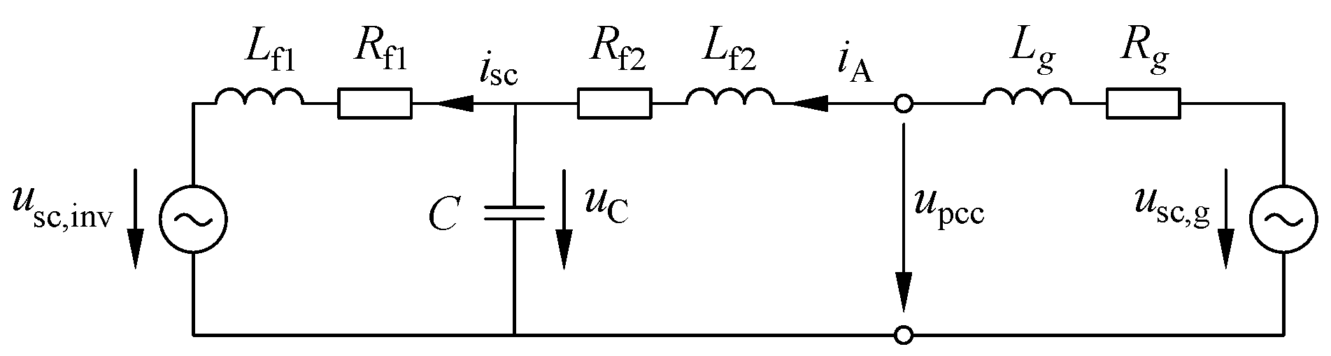
2.2. Two-Level Three-Phase LCL Inverter

The aim of this work is to define an inverter with an LCL filter as a method-specific component in the ENM in order to achieve a uniform model shape which can be used in this transient network calculation method. For this, the two-level three-phase inverter with an LCL filter pictured in Figure 1 shall be considered. For the sake of simplicity, the switches should be regarded as ideal.
Assuming symmetrical behavior, the three-phase circuit from Figure 1 can be simplified to one single-phase electric circuit diagram displayed in Figure 2, which represents each of the three single phases—a, b, and c.
It consists of a centered capacitance C, inverter-sided longitudinal impedance  L f 1  and  R f 1 , and grid-sided impedance  L f 2  and  R f 2 . The voltage directly at the switches’ outlet is defined as inverter source voltage  u sc  and the inner source current as  i sc . The quantities  i A  and  u A  are the terminal current and voltage. The A-terminal represents the point of common coupling (pcc) of the inverter, so that  u pcc = u A . Depending on the purpose of the specific investigation, two main inverter models are common practice [9,12]: the “switched” and “average model”. In terms of control design and dynamic analyses, average values become of higher interest in comparison to instantaneous values [9] and, hence, the average model is often sufficient. It is based on the moving average, describing the varying average value from one switching cycle to another. Using the average model, the time-dependent inverter source voltage  u sc ( t )  is formulated as a function of the sinusoidal modulating signal  m ( t ) . The two-level inverter’s source voltage  u sc , abc ( t ) , representing three-phase power supply at a DC link with voltage  U DC , can then be expressed as follows:
u sc , abc ( t ) = u sc , a ( t ) u sc , b ( t ) u sc , c ( t ) = m abc ( t ) U DC 2
with the modulation signal vector  m abc ( t ) , with  m a m b , and  m c , where  1 m ( t ) 1 . To keep the focus on the AC consideration,  U DC = const .  is assumed in the following.

2.2.1. LCL Filter Design

The main requirement of the inverter filter is the filtering of high frequencies caused by switching, so that the terminal current to be fed into the grid only has low harmonic distortion [1]; hence, the passive components must be selected according to the desired attenuation, especially at the switching frequency  f sw  and higher. Due to the central cross capacitor, LCL filters offer a path with low impedance for high frequencies. But this creates a resonance point, for which certain boundary conditions must be adhered to in order to maintain control stability. At the same time, the voltage drop across the filter should not be too great in order to avoid high power losses. Some universally applicable approaches on LCL filter design [1,2,3] especially depend on the switching frequency  f sw , the inverter’s nominal power  P n , and the considered grid voltage level  u n . Only if the filter fulfills the requirements for attenuating high-frequency parts can it be used as an average model for network calculations in the fundamental grid frequency  f 0 . Therefore, the chosen path in this work is briefly presented in the following, including the approaches in [1,2,3]. The maximum value of the total filter inductance  L tot = L f 1 + L f 2  is given as follows [1,3]:
L tot 0.1 U n 2 ω 0 P n
with the fundamental grid angular frequency  ω 0 . In [1], the factor for dividing the total inductance  L tot  between  L f 1  and  L f 2  defined as  α L = L f 1 L f 1 + L f 2  is given as being between 0.5 and 0.9. In [2], the ratio between grid-sided and inverter-sided inductance  a = L f 2 L f 1  is defined with  a max = L tot , max L f 1 1 . The maximum value of the capacity is often based on the maximum acceptable power loss due to reactive power according to [2]:
C < 0.05 P n ω 0 U n 2 .
In [1], it is recommended to estimate C from the desired damping at the switching frequency of between about 50 and 90 dB [1], while damping at the fundamental frequency  f 0  must be within an acceptable range. The harmonic attenuation rate
δ = 1 | 1 + a L ( 1 L f 1 C ω sw 2 ) |
with the angular switching frequency  ω sw = 2 π f sw  should be small to guarantee low current harmonics.  δ  is upwards limited due to the distance between the resonance frequency and cutoff frequencies  f c , min = f sw 6  and  f c , max = f sw 2 . Downwards, it is limited by the condition
δ > δ min = 1 | 1 + a max ( L f 1 C ω sw 2 1 ) | .
The resonance frequency  f res  of the LCL filter is given as
f res = 1 2 π L f 1 + L f 2 L f 1 L f 2 C .
It must be located between the minimum and maximum cutoff frequencies  f c , min  and  f c , max  [2], so that finally for the resonance frequency, the condition
10 f 0 < f sw 6 f res , min < f res < f res , max < f sw 2
must be fulfilled. In general, the derived design parameter can be checked for plausibility using the conditions
Z L ( f 0 ) Z C ( f 0 ) , Z C ( f sw ) Z L ( f sw )
with  Z L  stating the inductive longitudinal path and  Z C  the capacitive cross-branch [2].

2.2.2. Resonance Damping

As the stability of the inverter control suffers due to the existence of the resonance peak of the LCL filter, there are various ways of damping [3]. Two strategies for passive damping are the connection of a small damping resistor  R C  in series with the filter capacitance C or a very low conductance  G c  in parallel [3]. The damping resistance  R C  causes a shift of the resonant pole and provides a further zero in the filter transfer function [1]. In contrast, adding a parallel conductance to the capacitance does not affect the characteristics of the frequency response. But the disadvantages—large damping losses and poor reference tracking and disturbance suppression capability—are mentioned in [3].

2.3. LCL Inverter Model in the Extended Node Method

To make the inverter with the LCL filter applicable in the ENM, the corresponding valid equivalent circuit diagram is interpreted in the time-domain and transformed into a method-specific component equation. Here, a basic LCL filter as well as two cases with resonance damping are considered. The relevant parameters will be specified and it is mentioned where they are placed into the component matrices and vectors of the DAE in the Equations (3)–(5).

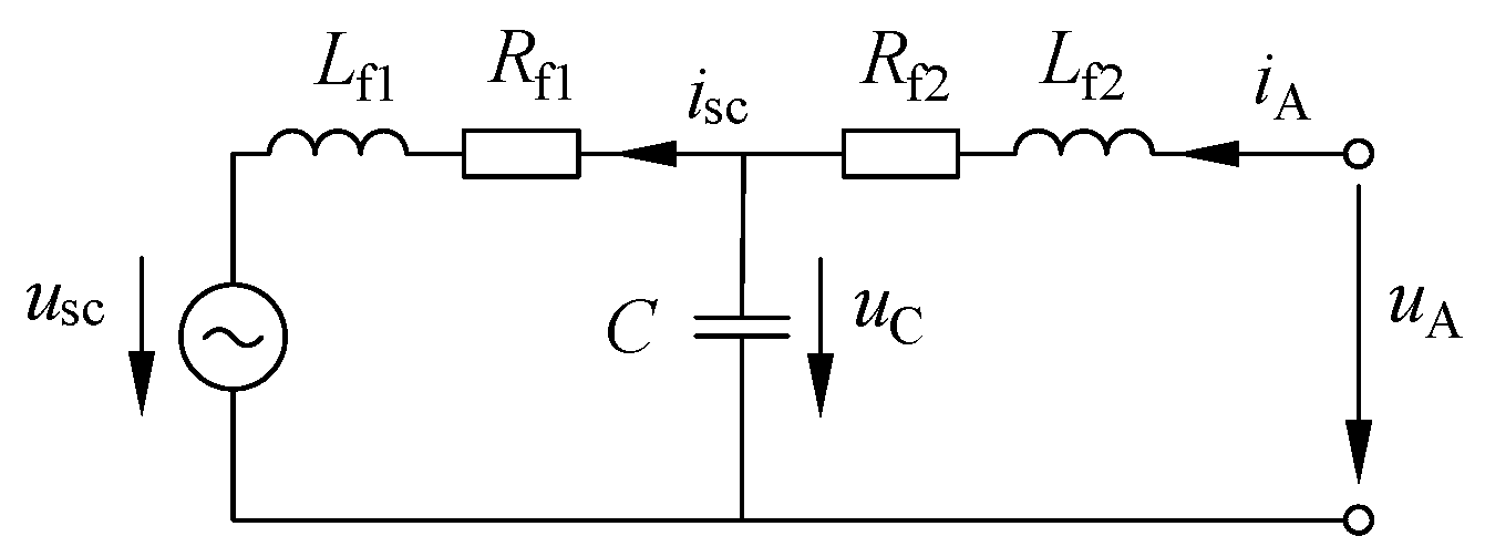
2.3.1. Basic LCL Inverter

The electric circuit diagram of the basic LCL filter neglecting damping resistors is displayed in Figure 2. The explicit equation of state for the grid-sided mesh is
L f 2 i ˙ A + R f 2 i A + u C = u A
and meets the definition of an L-A component in the ENM (cf. [37]). The typical conversion of Equation (14) for L components gives
i A = 1 ω 0 i ˙ A = 1 ω 0 L f 2 G L , G L , diag . u A 1 ω 0 L f 2 G L , G L , diag . ( R f 2 R L i A i L + u C u scL ) .
The grid-sided parameters  R f 2  and  G f 2 = 1 ω 0 L f 2  occur as scalar inputs for the system matrices in  R L  and  G L  and  G L , diag . , respectively, in Equations (3) and (4). The terminal current is part of the inductive current vector  i L  and therefore a result of the DES in Equation (4). As an L component, the LCL inverter is not the decisive component for node characterization (cf. (1)). This means that the node at the output terminals can be an L node as well as an R or C node if other component types (R or C) are connected ( u A u LN , u RN , or  u CN ). The source voltage  u scL  in the sense of the ENM is not the actual inverter source voltage but the capacitor voltage  u C . Hence,  u C  is inserted as an element into the vector  u scL  in Equations (3) and (4). This voltage  u C  in turn depends on the internal source current  i sc . The differential equations of the capacitance  u C  and the source current  i sc  are
u ˙ C = 1 C ( i A i sc )
i ˙ sc = 1 L f 1 ( R f 1 i sc + u C u sc ) .
Both variables are consolidated in the vector of inner variables
z LCL = u C i sc
and result in the IDES in matrix form corresponding to Equation (5), as follows:
u ˙ C i ˙ sc z ˙ = 0 1 C 1 L f 1 R f 1 L f 1 M z u C i sc z + 1 C 0 0 1 L f 1 M r i A u sc r .
The actual inverter’s source voltage  u sc  as well as the inverter-sided passive components  L f 1  and  R f 1  are not part of the actual grid DAE in Equations (3) and (4), but only occur in the IDES in Equation (5).

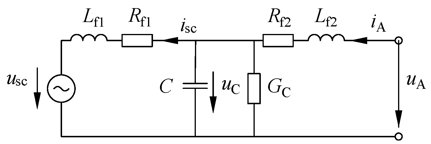
2.3.2. LCL Inverter with Parallel Damping Resistor

If a conductance  G C  is arranged parallel to the central capacitor for resonance damping and should not be neglected, the electric circuit diagram of the inverter with LCL filter is created as shown in Figure 3.
Thereby, Equation (17) is modified to
u ˙ C = 1 C ( i A i sc ) G C C u C
which states an additional entry in  M z  so that Equation (19) is modified to
u ˙ C i ˙ sc = G C C 1 C 1 L f 1 R f 1 L f 1 u C i sc + 1 C 0 0 1 L f 1 i A u sc .
Since Equation (15) still describes the behaviour of the grid-sided mesh, the definitions of the component type as well as the system parameters for  R L G L  and  u C u scL  do not change compared to the basic LCL filter.

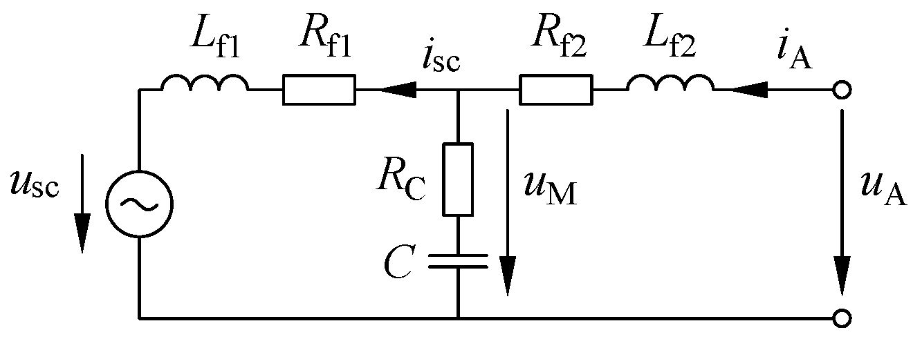
2.3.3. LCL Inverter with Series Damping Resistor

Considering a damping resistor  R C  in series to the centered capacitor, the electric circuit diagram of the inverter with LCL filter is changed to the one displayed in Figure 4.
Due to  R c , the internal voltage no longer exhibits purely capacitive behavior, but now consists of capacitive part  u C  and resistive part  u R , so that  u M = u C + u R  states the new resulting voltage over the cross branch. By this, Equation (22) is adapted to
i A = 1 ω 0 i ˙ A = 1 ω 0 L f 2 G L , G L , diag . u A 1 ω 0 L f 2 G L , G L , diag . ( R f 2 R L i A i L + u M u scL ) .
This does not affect the characterization of the inverter component type, which is still an L-A component. But in this case,  u M  represents the source voltage in the vector  u scL . The differentially behaving quantities  u C  and  i sc  shall still be sorted in  z . Taking into account the now additionally acting voltage  u R = R C ( i A i sc )  affecting  i sc , Equation (19) is changed to
u ˙ C i ˙ sc = 0 1 C 1 L f 1 R f 1 + R C L f 1 u C i sc + 1 C 0 R C L f 1 1 L f 1 i A u sc .
Keeping the structures of  z  and  r u M  can be determined with
u M = 1 R C M z , alg u C i sc + R C 0 M r , alg i A u sc
and, so to speak, represents an additional inner AES, which also must be evaluated at every timestep just like the Equations (3)–(5).

2.3.4. Sensitivity of Filter Parameters

In the following, it will be briefly described how the values of filter inductances  L f 1  and  L f 2  and of the capacitor C affect the system matrices and hence the computation outcomes of the ENM. The general design should fulfill the criteria mentioned in Section 2.2.1, but the actual values in operation may differ slightly from the design values, or the availability of components may not correspond to the exact design values. Therefore, it makes sense to also consider close values around the design point, to evaluate if the inverter operation is stable with the selected control strategy, even with small deviations in the filter parameters. Hence, it will be briefly addressed how changes around the exact design parameters  L f 1 L f 2 , and C affect the system quantities and the matrices for the grid calculation with the ENM for the basic LCL inverter model. The modified values are defined as  L ˜ f 1 = ζ f 1 L f 1 L ˜ f 2 = ζ f 2 L f 2 , and  C ˜ = ζ C C  with the gain factors  ζ f 1 ζ f 2  and  ζ C > 0 . The LCL inverter component Equation (15) and the IDES of Equation (18) can then be written as follows:
i A = 1 ω 0 i ˙ A = 1 ω 0 ζ f 2 L f 2 G L , G L , diag . u A 1 ω 0 ζ f 2 L f 2 G L , G L , diag . ( R f 2 R L i A i L + u C u scL ) ,
u ˙ C i ˙ sc z ˙ = 0 1 ζ C C 1 ζ f 1 L f 1 R f 1 ζ f 1 L f 1 M z u C i sc z + 1 ζ C C 0 0 1 ζ f 1 L f 1 M r i A u sc r .
In general, the impedance decreases for the grid-sided LR branch for  ζ f 2 < 1  and increases for  ζ f 2 > 1 . For small impedance, the terminal current increases in its root mean square value. Due to the increasing absolute values of the prefactors for  ζ f 2 < 1  prior to  u A R f 2 i A , and  u C  in Equation (25), the influence of the individual variables on the current derivative increases accordingly in a linear manner. These prefactors are part of the component conductance matrices  G L  and  G L , diag . , which occur frequently in the matrices of the DAE in the Equations (3) and (4). Depending on whether the LCL inverter is connected to an L, R or C node, the node conductance matrix  G LL G LR  or  G LC  is also affected. When considering the inverter-sided LR branch of the LCL filter, the same applies to the current derivative  i ˙ sc  of the source current when varying the filter inductance  L f 1 . For  ζ f 1 < 1 , the absolute values of the matrix entries in the second row of  M z  and  M r  become larger; thus, the influence of the corresponding quantities increases linearly. For  ζ f 2 > 1 , the matrix entries become smaller in their absolute values. According to the definition of the LCL inverter with internal variables, a variation of the filter inductance  L f 1  only affects the IDES in Equation (5), but not the DAE in Equations (3) and (4). By varying the capacitance, the cross-branch impedance is reduced for higher values and increased for lower values of C. Here, too, the absolute values of the matrix entries in the first row in  M z  and  M r  become higher for  ζ C < 1  and describe the voltage derivation  u ˙ C . Changes to C also only affect the matrices of the IDES in Equation (5).

2.3.5. On Solving Inner Differential Equation Systems vs. Stating Additional Grid Nodes

As could be observed from the previous sections, when considering an inverter with an LCL filter as an L-A component, internal state variables are present. These are the capacitor voltage  u C  and the internal source current  i sc . They have to be solved with the help of the IDES according to Equation (5)—more precisely, with the help of Equations (19), (21), and (23). In the case of an LCL filter with a series damping resistor, the capacitor voltage  u C  only represents a part of the actual centered voltage  u M , which states the source voltage in  u scL , and thus even an additional algebraic equation, Equation (24), is found, which has not yet been considered with any classic component in the ENM so far (cf. [36]). In order to avoid these internal state variables for the LCL filter, it is also possible to organize the LCL filter differently by dividing it into further individual components. Since generally good experiences have been made with the application of the IDES in Equations (19), (21), (23), and (24), this possibility will only be briefly described in the following to generally enable this method of application.
The inverter-facing LR series branch would represent an L-A component itself with the source voltage  u sc u scL  and the grid-facing series impedance of  L f 2  and  R f 2  indicates an L-AB component, whose parameters have to be arranged in matrix form. Particular attention should be paid to the diagonal form and complete form of the conductance ( G L  and  G L , diag , cf. Section 8.2.2 in [36]). The central capacitor is to be defined as a C-A component with  G C = 0  for the basic LCL filter and the one with the parallel conductance as  G C 0 . This makes the inner node of the filter a C node by definition for the ENM. Its node voltage is now part of  u CN  and a result of the DES in Equation (4). In the case of a series damping resistor  R C , an R-AB component is also added and characterizes the central node of the filter as an R node. The node voltage acting here corresponds to the previously defined  u M . It is part of  u RN  and results from the AES in Equation (3). The node between  R C  and C is by definition a C node. Its node voltage will be part of  u CN .
This decomposition of the LCL filter into its individual parts generally increases the number of grid components and nodes, thereby also increasing the size of the DAE. But advantageously, the IDES is either eliminated completely or limited to other network components, such as transmission lines represented by T or Pi-EC (cf. [36]). The favourable approach remains the decision of the user. When choosing the approach with the internal variables, it is recommended to keep the uniform shape of Equation (5) for all components with inner state variables and also the sorting of the components, so that they can be easily put together in large diagonal matrices  M z  and  M r . In the application example used here, the basic LCL filter model is used as an L-A component with the IDES.

2.4. Inverter Control

In this section, a control algorithm in the dq frame will be applied to later show how it can be included in the ENM in Section Combined Control and Grid Calculation Algorithm. Using the rotating dq frame for inverter control is advantageous, because the variables to be controlled gain the shape of DC quantities, which allows the use of simple PI controllers [9]. As already mentioned, several investigations already exist on the inverter control with LCL filters. The aim of this work is not to propose a new control strategy, but to show how the inverter control loop interacts with the ENM. From this, the effects of inverter control on the grid can be analyzed in order to evaluate the stability or to try out suitable controller parameters. The “measured” variables for the control loops occur directly during the calculation. This is independent of the number of inverters under consideration, so it can be performed for networks with numerous connected power-controlled inverters. The application of the inverter control loop is not limited to the following example. Rather, any type of control can be used.
In the following sections, it is briefly shown how current references are obtained from power references in the dq frame. Subsequently, an example of a cascaded current control loop for the inverter is presented. Finally, a PLL example is given, which is used in this work.

2.4.1.  P Q  Control in dq Frame

The active and reactive power P and Q of the inverter are to be controlled at the pcc; hence, the dq frame is defined there. For the conversion between abc and dq variables, the amplitude invariant transformation matrices  T abc , dq ( θ )  and  T dq , abc ( θ ) , defined as
T abc , dq ( θ ) = 2 3 cos ( θ ) cos ( θ 2 π 3 ) cos ( θ 4 π 3 ) sin ( θ ) sin ( θ 2 π 3 ) sin ( θ 4 π 3 ) ,
T dq , abc b c ( θ ) = cos ( θ ) sin ( θ ) cos ( θ 2 π 3 ) sin ( θ 2 π 3 ) cos ( θ 4 π 3 ) sin ( θ 4 π 3 )
are used. The time-dependent angle  θ  states the angle between the fixed  α β  coordinate system and the rotating dq frame [9]. Since the electric grid behind the pcc can have any shape, it is advantageous to define the fed-in power on the basis of the inverter’s terminal values  u A  and  i A . According to the introduced sign convention in Figure 2 P pcc  and  Q pcc  are formulated from dq quantities as
P pcc ( t ) = 3 2 ( u pcc , d ( t ) i A , d ( t ) + u pcc , q ( t ) i A , q ( t ) )
Q pcc ( t ) = 3 2 ( u pcc , d ( t ) i A , q ( t ) u pcc , q ( t ) i A , d ( t ) )
with the terminal currents  i A , d  and  i A , q  and pcc voltages  u d , pcc  and  u q , pcc . For  u q , pcc = 0 , as desired in the PLL [9] (cf. Section 2.4.3), the current references  i A , d *  and  i A , q *  can be obtained with the help of the power references  P *  and  Q *  [9]:
i A , d * = 2 P * 3 u d , pcc ,   i A , q * = 2 Q * 3 u d , pcc
and will be used in grid current control as the reference variable.

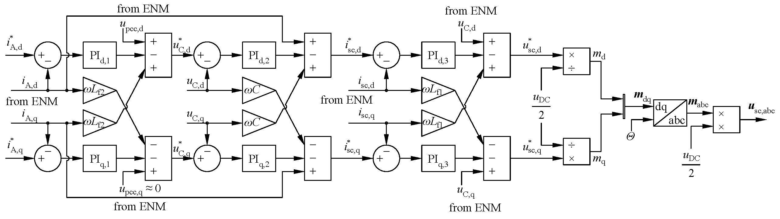
2.4.2. Current Control

The cascaded current controller shown in Figure 5 with disturbance feed-in will serve as an example for current control of an inverter with an LCL filter. It is mainly created for the basic case of the LCL filter—i.e., damping resistors are neglected ( R C = 0  and  G C = 0 ). By using the cascaded approach, mainly inspired by [21], the system is broken down into three first-order systems [1], thereby simplifying the design of the individual controller parameters. The control here is implemented in the time domain. For this purpose, each PI controller output signal  o u t ( t )  is discretized to be
o u t ( t ) = K p e ( t ) + K i e ( t ) t t 1
with the error signal  e ( t ) , the proportional gain  K p , integral gain  K i , the current point in time t, and the previous point in time  t 1 .
The current setpoints  i A , d *  and  i A , q *  resulting from Equation (31) serve as the reference inputs. The terminal currents in the abc frame result from  i L  in Equation (4). They are transformed into dq quantities  i A , d  and  i A , q  and fed into the control loop as control variables. The controller outputs of  PI 1 , d  and  PI 1 , q  are used to generate the reference values for the filter capacitance voltages  u C , d *  and  u C , q * . In the following, the source current references  i sc , d *  and  i sc , q *  are obtained and the error between them and the actual values  i sc , d  and  i sc , q  go into the third PI controller  PI 3 , d  and  PI 3 , q . Finally, the control loop sets the modulating signals  m d q , which can be retransferred to the abc frame and used to set the inverter’s source voltage  u sc , d q *  according to Equation (6). For simplicity,  u sc = u sc *  is set here. Figure 5 already indicates that the variables  i A u pcc u C , and  i sc  to be introduced into the control loop are extracted from the ENM. Finally, the structure of the software tool for grid calculation with the ENM is described and a detailed insight into the methodical design of the handover between inverter control and grid calculation is given in Section Combined Control and Grid Calculation Algorithm.

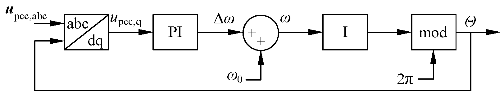
2.4.3. Phase-Locked Loop

To keep the quadrature axis reference  u pcc , q  at the pcc at zero for grid synchronization, a synchronous reference frame PLL loop according to Figure 6 is applied [9,49]. Beyond this introduced PLL algorithm, any type of PLL is conceivable in combination with the LCL inverter model and the ENM.

2.5. Software Tool for Transient Grid Calculation with ENM

Before the actual transient calculation takes place, all grid components and nodes are created with the help of Python using object-oriented programming. The components are sorted by L, R, and C components as proposed in [36]. Within each group, the components are also sorted according to their number of terminals (A and AB). The parameters of the sorted, uncoupled components set up the system matrices  G L  and  R L  for L components,  G R  for R components, and  C C  and  G C  for C components [36]. For components with inner state variables, especially the inverter with the LCL filter in this work, the matrices  M z  and  M r  are also built. These matrices are joined in such a way that a large IDES of the form given in Equation (5) is created. In case of the inverter with a series damping resistor,  M z , alg  and  M r , alg  are also to be constructed. By connecting components to the nodes, these are classified according to the definition given in (1) as L, R, or C nodes. The nodes are also sorted accordingly and all clamping matrices  K  (cf. Equation (2)) are constructed. The node conductance matrices  G LL G LR G LC G RR G RC G CR , and  G CC  and the node capacitance matrix  C NN  are determined using the  K  matrices and component matrices (cf. [36]). With this, all matrices can be set up for the DAE in the Equations (3) and (4). In the work shown here, a three-phase symmetrical calculation is carried out. Initial values for the node voltages and terminal currents can be determined using complex AC calculations for steady-state conditions.

Combined Control and Grid Calculation Algorithm

A visualized representation of the ENM algorithm for transient grid calculation using the DAE in Equations (3) and (4) is given in Figure 7 taken from [36]. The Box ‘Algebraic Node Voltage Equation’ represents the AES with the node voltages at L and R nodes  u LN  and  u RN  as its outputs. The boxes ‘L Components’ and ’C nodes’ define the DES. The ‘L component’ box provides the results of the inductive currents  i L  and the ‘C node’ box delivers results of the node voltages  u CN  at C nodes.
To show how the inverter with the LCL filter with subordinate control can be included in the ENM, the illustration in Figure 7 has been expanded with the box ‘LCL Inner States’ and the handover points of the variables to the inverter control loop. Hence, Figure 7 pictures the combined network calculation/control algorithm. In this work, this combined algorithm was implemented in the Julia language using the ‘DifferentialEquations.jl’ package.
For reasons of clarity, the abc/dq conversion is not explicitly shown. But in general, an abc/dq conversion takes place at any point indicated with ‘to Controller’. The schemes of the control loop in Figure 5 and the PLL in Figure 6 are written as functions in Julia using Equation (32) for the PI controllers. Their algorithms and hence the setting of the new inverter source voltage  u sc  are only carried out at times that are multiples of  T ctrl = 1 f c t r l , while the numerical integration of the DES and IDES is carried out in smaller time steps. The illustration was developed based on the cascaded controller in Figure 5, but generally applies to all control approaches that require the same or fewer state variables as inputs. In this case, a particularly large number of input variables from the network calculation is required ( i A u A u C , and  i sc ) and hence this is an example of a particularly strong exchange between the network calculation process and the controller algorithm. Fortunately, all necessary variables occur as a solution at every time step anyway during the solving process.
Since the LCL filter is an L component, its terminal current  i A  can be extracted as a part of  i L . It is fed into the current controller as the controlled variable, but also states a part of  r  to be put into the ‘LCL Inner States’ box representing the IDES in Equation (19) for the LCL filter. Another necessary input of this box is the inverter source voltage  u sc , which results from the control loop. The pcc voltage can be extracted out of one of the node voltage vectors  u LN u RN , or  u CN . It is needed for the PLL as well as for the current control loops as the disturbance input. The output of the ‘LCL Inner States’ box is the vector  z LCL  containing the inner capacitor voltage  u C  and the source current  i sc u C  is extracted to be put into  u scL , which is needed as an input for the boxes ‘Algebraic Node Voltage Equation Voltage’ and ‘L components’.
It should be emphasized again that any other inverter control loop can also be combined with this grid calculation method to check on the robustness or speed of controller designs at various grid topologies. Further compensators, observers, and pre-filters can also be inserted between the grid calculation results and the controller. Also, it is not limited to the grid-following mode.
When considering large power grids, many other grid components occur. In addition, further internal state variables  z  arise, in particular for power transmission lines (cf. [36]). However, in order to keep the focus on the LCL filter, further internal state variables are not explicitely shown in Figure 7.

3. Results

To ensure that the ENM with the developed inverter component and subordinate control loop developed here can be used for transient grid calculations, its accuracy and reliability must be verified. For this purpose, various study cases of inverters connected to a European low-voltage grid ( U n = 400  V,  f 0 = 50  Hz) are considered. Firstly, the filter design selected here is presented. Subsequently, grid calculations are carried out with the ENM using the DAE given by Equations (3)–(5) and the established tool Simulink/Simscape as comparison software. Thus, the same grid configurations are set up once in our own tool according to the ENM’s component and node definitions (cf. Section 2.5) and once in Simulink (Matlab R2024b) using the Simscape ‘Specialized Power Systems’ library [50]. The inverter control loops are also set up in the same way according to Figure 5, realized by interconnecting single blocks available in Simulink. To focus on the inverter component, transients are generated by changing the power references  P *  and  Q *  as an ideal step function, while the loads are kept constant. This work does not take into account how the power references  P *  and  Q *  are derived, but specific methods can also be easily supplemented here. They could, for example, be the result of maximum power point tracking of PV systems or result from economic optimization for the operation of electrochemical components or batteries or from grid code requirements. Both results will be compared in the following sections. The ENM results will be displayed with a solid line and not specially marked. Simulink results will be shown with a dashed line and marked with ‘Sim’ in the index. Further discussion on the results and the presented method will be given in Section 3.4.

3.1. Filter Design and Control Parameters

According to the mentioned LCL filter design requirements in Section 2.2.1, one sample filter design is given in Table 2 that meets the requirements for the switching frequency  f sw = 20  kHz. It will be used for the following study cases. In this case, the controller parameters are designed for a fast response. A damping resistor is neglected; i.e., the following results are based on the basic LCL model from Section 2.3.1. The resulting Bode diagram of this filter design is pictured in Figure 8. The transfer function for the design selected here is plotted with the exact values from Table 2 as well as with 20% deviating values for  L f 1 L f 2  and C in order to take the component tolerances into account. For the configuration selected here, the distance of the resonance frequency to the cutoff frequencies  f c , min = 3.333  kHz and  f c , max = 10  kHz is maintained.
Selected controller parameters for the PLL and the current control loop are also listed in Table 2. In order to stabilize the inverter control by slightly decoupling it from the AC network dynamics [9], feed-forward compensation for the  U pcc , dq  is introduced. This is implemented as a low-pass of the form
U ˜ pcc ( t ) = U ˜ pcc , 1 + ( KU pcc ( t ) U ˜ pcc , 1 ) d t τ + d t
with time-constant  τ  and  d t = t t 1 . The values  U ˜ pcc , d  and  U ˜ pcc , q  are applied to calculate the current references with Equation (31) and are fed into the control loop in Figure 5 as disturbance input.

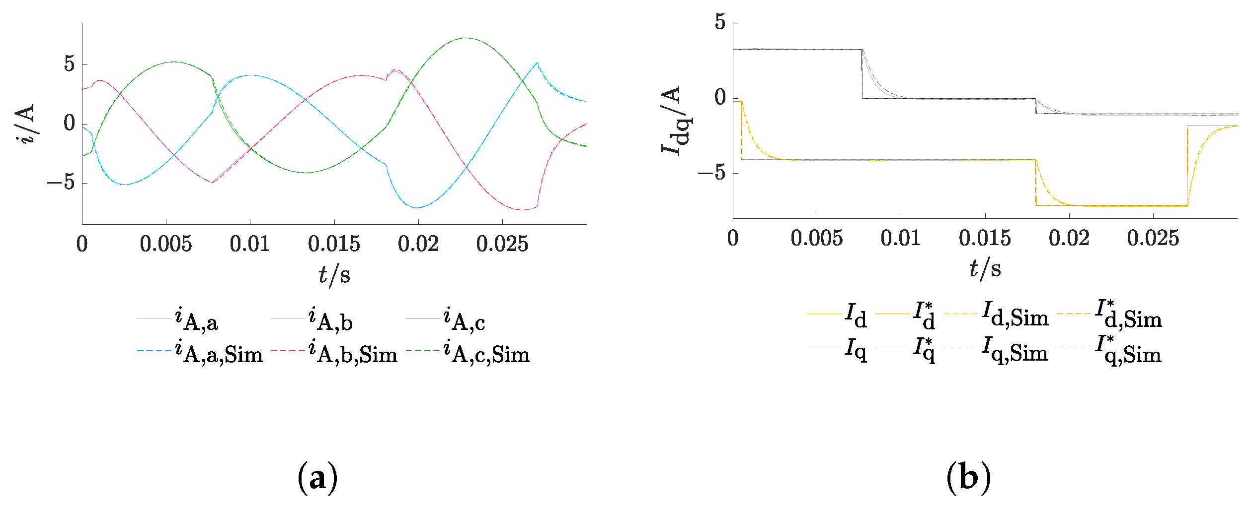
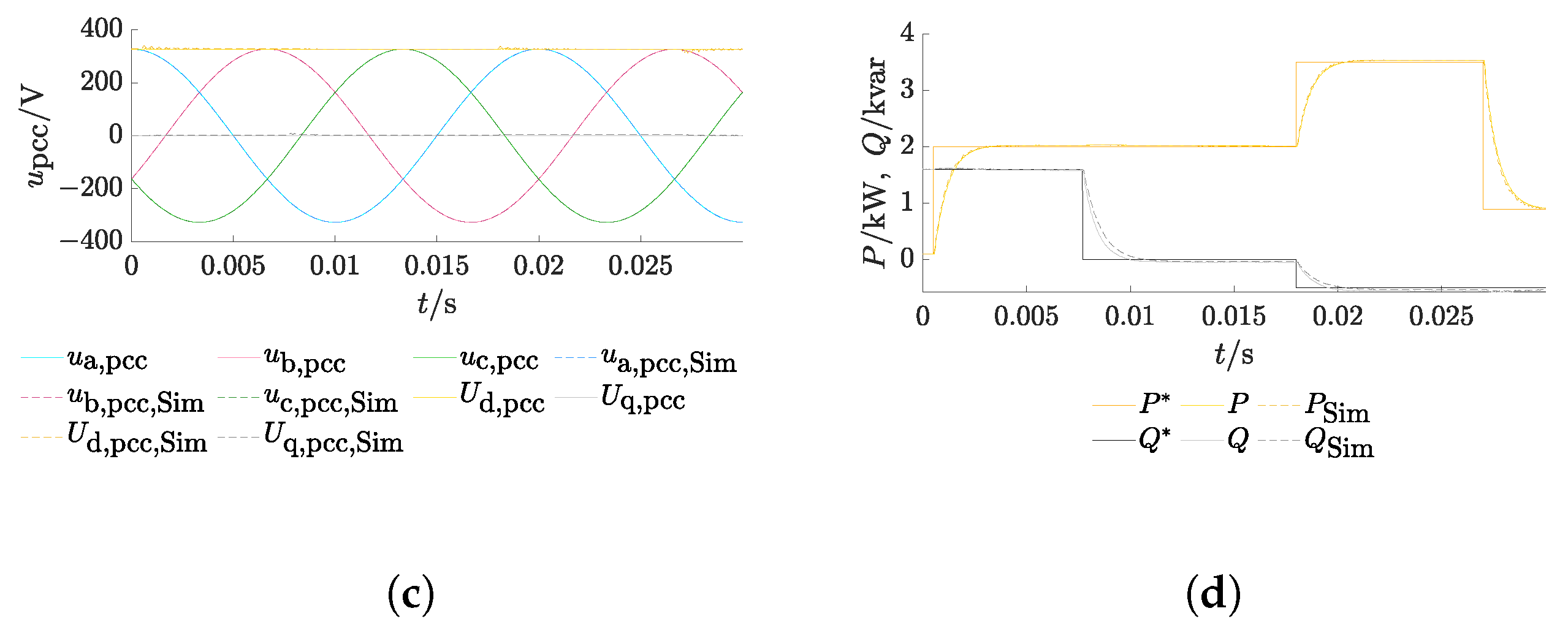
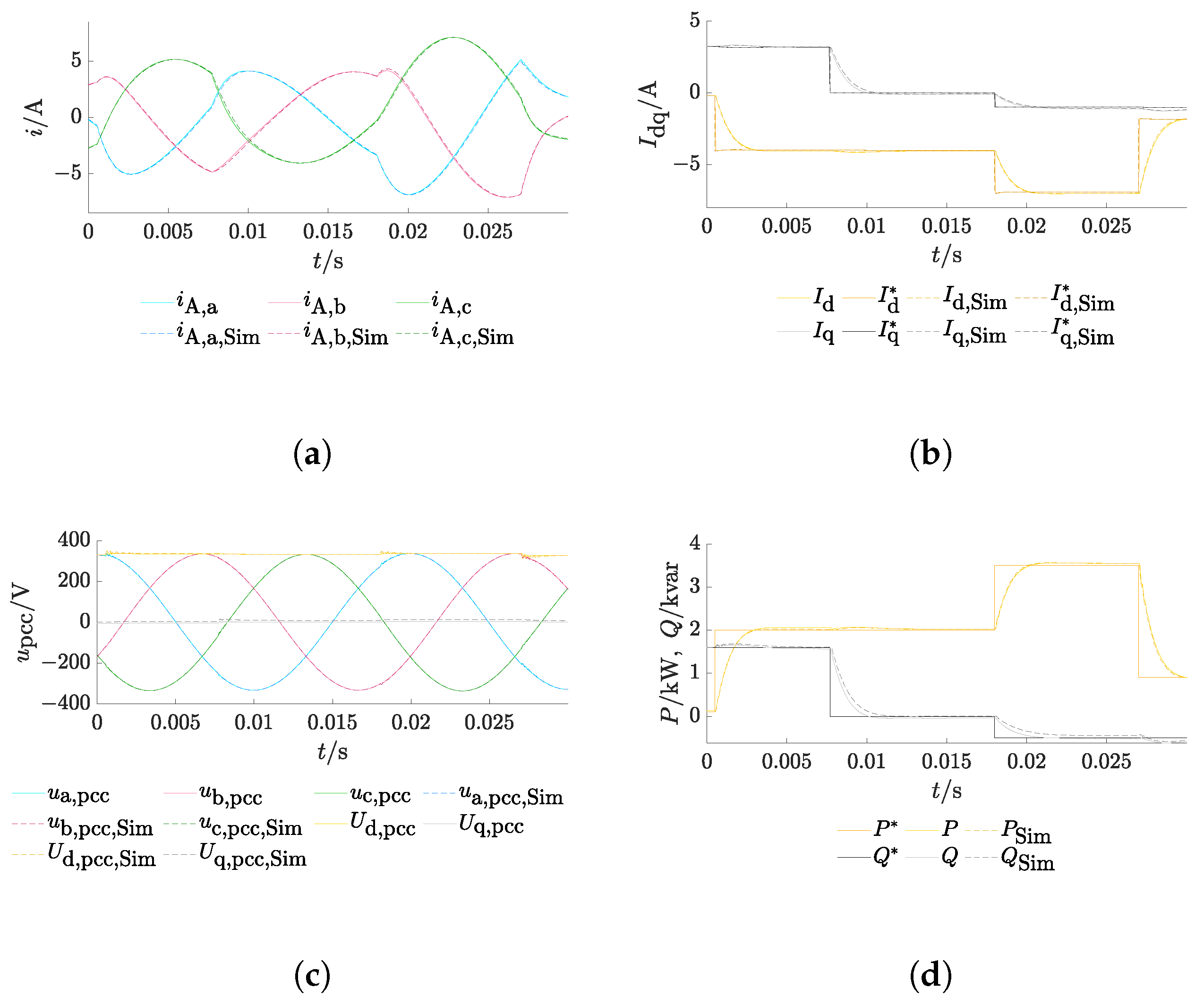
3.2. Single Inverter at Low-Voltage Grid

Firstly, one single inverter model is tested at a rigid low-voltage grid. The single-phase electric circuit diagram of the configuration is shown in Figure 9. The low-voltage grid is represented by an ideal voltage source with an LR series impedance. In this configuration, only one L node is present which states the pcc. Its node voltage is hence a part of  u LN  and will be determined by Equation (3).
In order to test the behavior of the grid-tied inverter and accuracy of the method for different grid impedances, three different values for  L g  and  R g  will be considered in the following with a constant R/X ratio of 2.4. For one case, Section Impact of Filter Parameter Deviations also displays an example of how small changes in the filter parameters affect the inverter operation. The power setpoints are changed according to the following cases:
P * ( t ) = 0.1 kW , t 0 s 2 kW , t 0.0005 s 3.5 kW , t 0.018 s 0.9 kW , t 0.027 s ,   Q * ( t ) = 1.6 kvar , t 0 s 0.0 kvar , t 0.0077 s 0.5 kvar , t 0.018 s .
Figure 10 shows the step responses of the system for a small grid impedance with  L g = 0.16  mH and  R g = 0.12 Ω , which represents a strong grid. In Figure 10a,b, the inverter terminal currents in the abc and dq frames, respectively, are presented. Figure 10c,d show the pcc voltage as well as the grid power values P and Q in comparison to the setpoints  P *  and  Q * . With the selected controller parameters, the step responses of the currents are very fast (cf. Figure 10b). In addition, the results between the ENM and Simulink agree very well, as no significant deviations can be observed. The phase currents match very well; only in the q component  I q  of the inverter current is a small difference visible at the transients, but this hardly affects the time constant of the step response. This small deviation is transferred accordingly to the transients of reactive power Q.
The corresponding results for higher grid impedance values  L g = 2  mH and  R g = 1.51 Ω  are displayed in Figure 11. Here, too, the instantaneous values of the two tools show good accordance and the step responses are fast. In Figure 11c, it can be seen that the q component of the pcc voltage shows a stationary deviation from its counterpart and is always slightly higher in Simulink. This also generates a small deviation in the reactive power from the target reactive power in Simulink, as can be seen in Figure 11d.
In Figure 12, the results are pictured for a grid impedance of  L g = 8  mH and  R g = 6.03 Ω , hence indicating a weaker grid. In this case, the problem of the interaction of PLL and current control mentioned in [23] can be observed. The P and Q step responses become significantly more shapeless, but generally show the same curve in both tools (cf. Figure 12d). Differences between the results of the ENM and Simulink occur slightly in the currents’ small phase shift in Figure 12a and at the pcc voltage  U q , pcc  in Figure 12c. This also affects a deviation in the reactive power curve.

Impact of Filter Parameter Deviations

Since the values of inductors and capacitors have tolerances and may fluctuate to some extent, an example of the previously presented second case with the grid impedance values  L grid = 2  mH and  R grid = 1.51 Ω  with varying filter parameters  L f 1 L f 2 , and C by a  ± 20 % change will now be considered. According to Section 2.3.4, this corresponds to the factors  ζ f 1 ζ f 2 , and  ζ C  being 1.2 or 0.8, respectively. For reasons of clarity, the following results will only be given for the cases if all filter parameter values increase ( L ˜ f 1 = 1.2 L f 1 L ˜ f 2 = 1.2 L f 2 , and  C ˜ = 1.2 C ) or decrease ( L ˜ f 1 = 0.8 L f 1 L ˜ f 2 = 0.8 L f 2 , and  C ˜ = 0.8 C ). The design case ( ζ f 1 = 1 ζ f 2 = 1 , and  ζ C = 1 ) is also printed for comparison. As the parameters here change to the same extent, only the substitute variable  ζ  will be used in the following. The setting of the control loop in Figure 5 as well as the feed-forward compensation should remain unchanged (cf. Table 2); hence, the controller parameters  K p  and  K i  for all three controllers as well as the gain factors still correspond to the design case. Figure 13 shows the time curves of the phase current  i A , c , the dq currents  I d  and  I q  of the inverter, and the active and reactive power references  P *  and  Q *  and actual values P and Q for varying  ζ . The results are compared again with Simulink, illustrated with a dashed line-style. To better visualize the impact of  ζ , only the time range from  t = 0  s to  t = 0.012  s is displayed.
For small  ζ  and thus smaller values for the inductances and the capacitor, steeper courses of the sinusoidal terminal currents occur, as can be seen here for  i A , c  in Figure 13a. With  ζ = 0.8 , steeper curves also arise for the dq currents  I d  and  I q  in Figure 13b and active and reactive power P and Q in Figure 13c after changes in power setpoints. The plots of the curves generated by Simulink show the same effects as the ENM. Since the gain factors in the control loop (cf. Figure 5) do not exactly match the component parameters  L ˜ f 1 L ˜ f 2 , and  C ˜  for  ζ 1 , steady-state deviations occur for active and reactive power compared to the reference values, but the system remains stable during inverter operation.

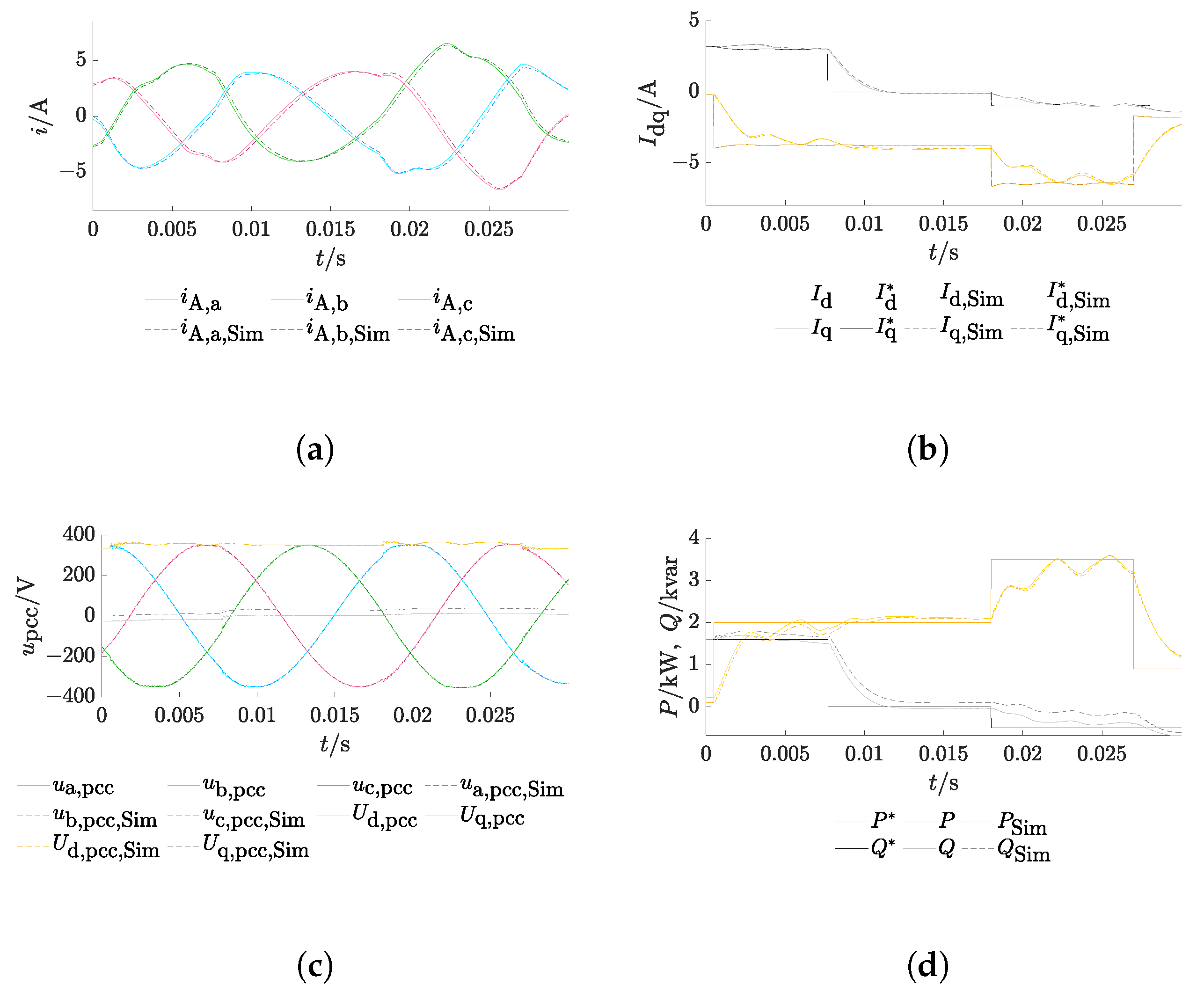
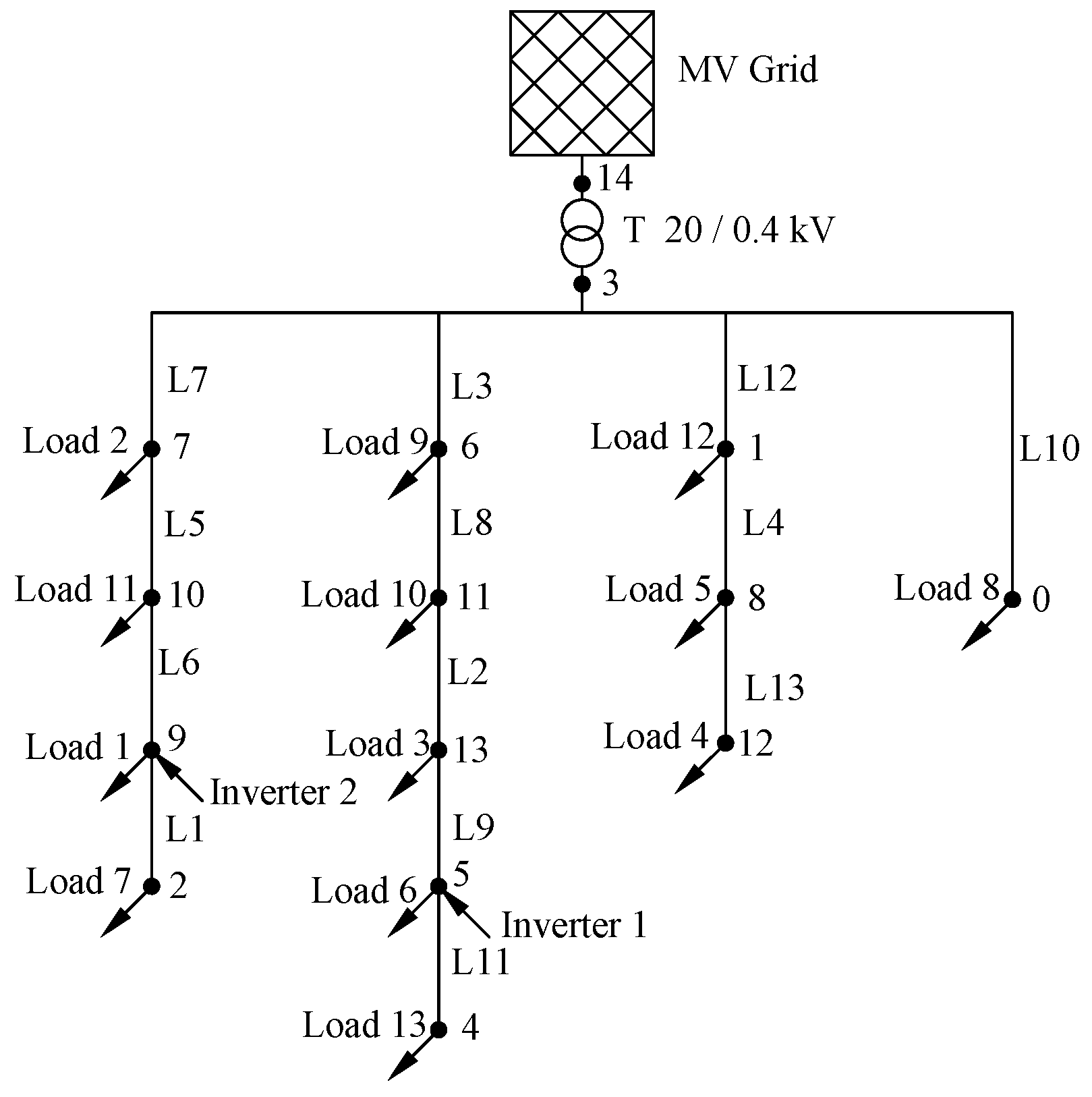
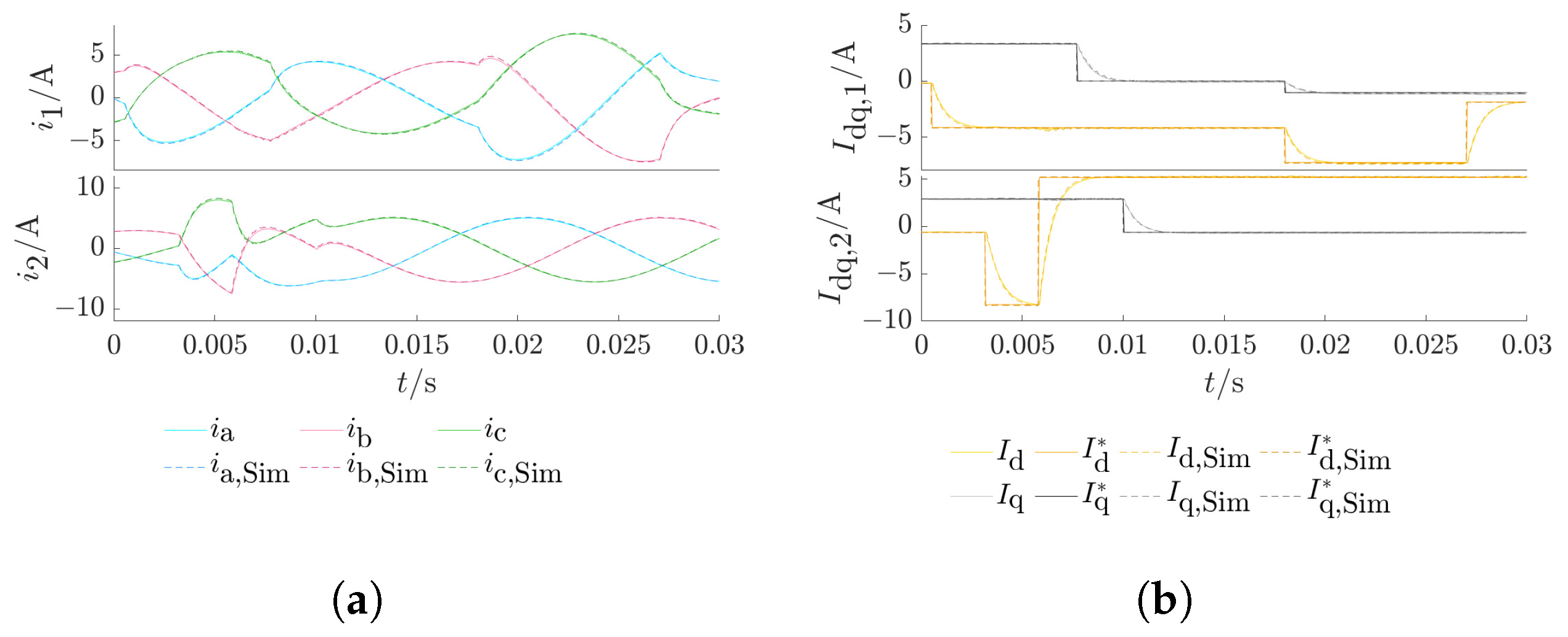
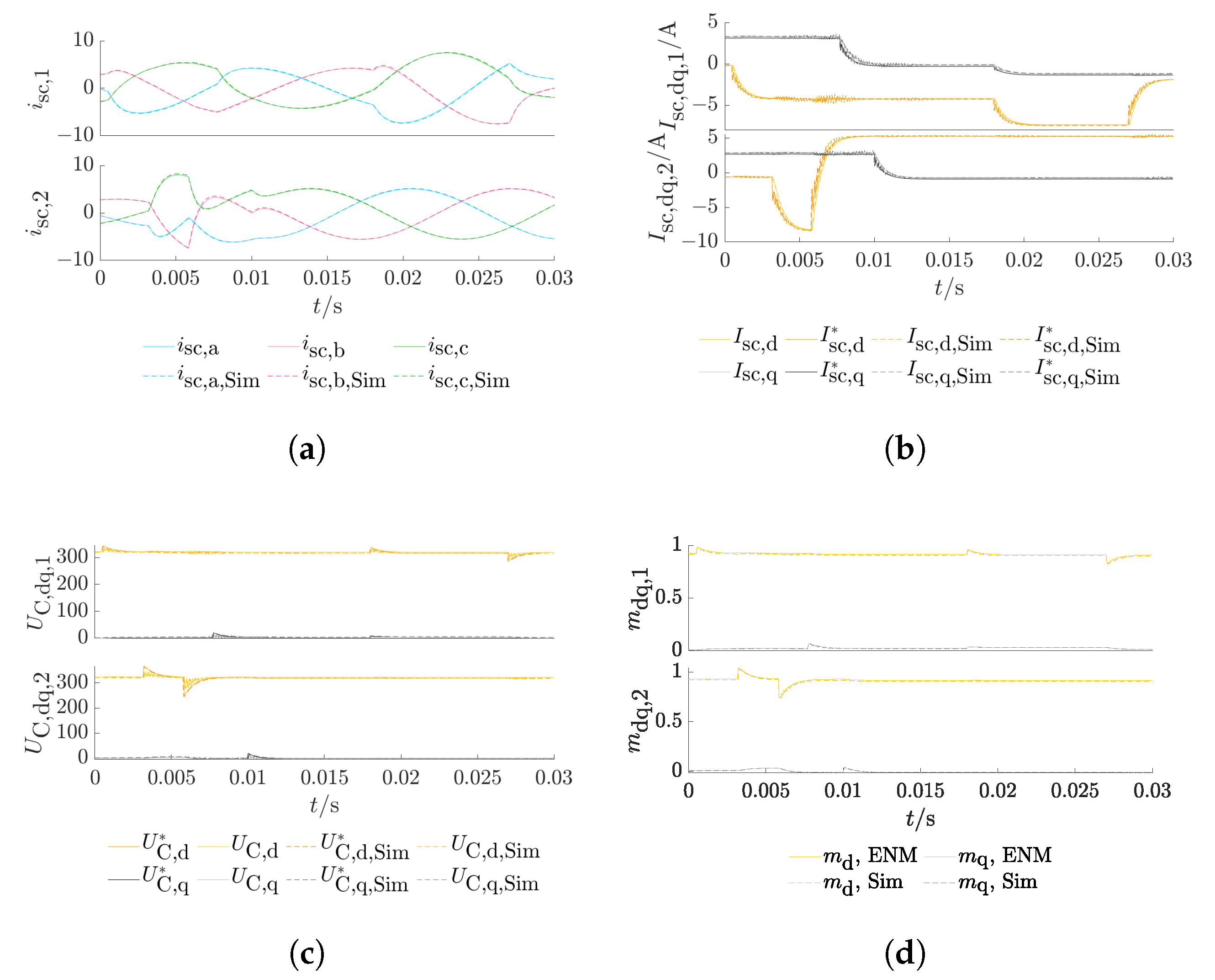
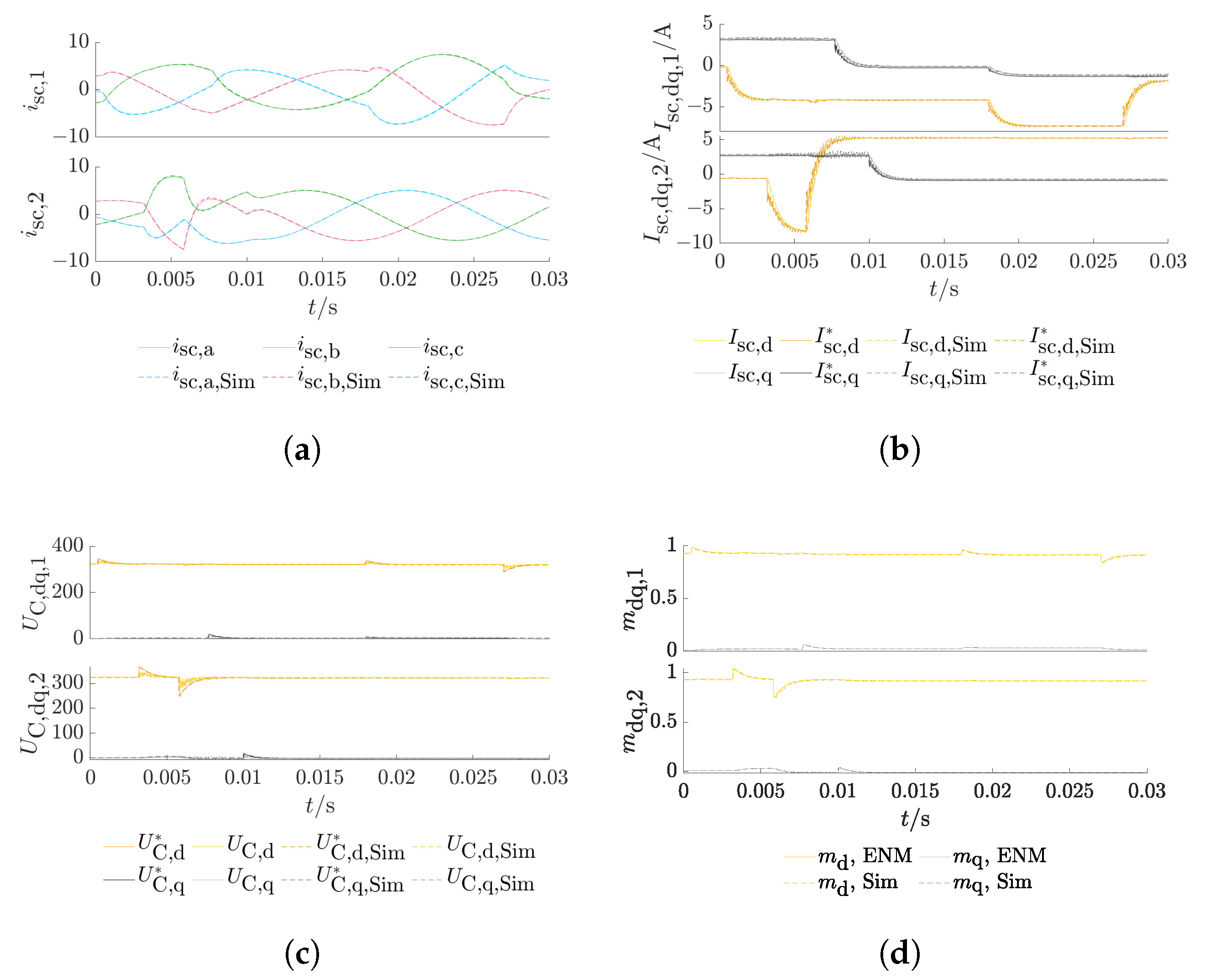
3.3. Inverters at Simbench Testgrid

Now, two inverters in the sample LV grid Simbench ‘1-LV-rural1’ as stated in Figure 14 will be considered. This testgrid consists of 15 nodes (0–14), 13 lines (L1–L13’), 13 loads (Load 1–Load 13) in the LV level, a medium-voltage (MV)/LV transformer, and a 20 kV MV grid. The LV section is exactly obtained from the network topology of Simbench ‘1-LV-rural1’, available at [51]. Further technical parameters for the transformer and the MV grid are summarized in Table 3. The transformer inductor  L s  and resistor  R s  are related to the secondary side (LV).
The power lines are modeled as a T electric circuit diagram, which correspond to L-AB components with inner capacitor voltages  u C , line  (cf. [36]), which become part of the vectors  z  and  u scL . The transformer model is simplified to an LR series element and also declared as an L-AB component. Two grid-synchronous inverters, labeled ‘1’ and ‘2’, are added at nodes 5 and 9.
In order to also represent the loads as electric circuit diagrams, impedances are used. Two different load situations are considered for this:
  • Study case 1: All loads (1–13) are resistive–inductive.
  • Study case 2: Loads 1, 6, and 11 behave capacitively; all other loads are resistive–inductive.
The individual load parameters  L load R load C load , and  G C , load  are listed in Table 4 for both study cases.
The resistive–inductive loads are each modeled as LR series impedances resulting from  L load = Q load U n 2 ω 0 ( P load 2 + Q load 2 ) , and  R load = P load U n 2 ( P load 2 + Q load 2 ) . The capacitive loads are modeled as CR parallel circuits and their values are determined by  C load = | Q load | ω 0 U n 2  and  G C , load = P load U n 2 . With T electric circuit diagrams for the lines, inductive loads, and also the LCL inverters as L components, the network only consists of L components for study case 1. Since there are no components of type R or C, no R or C nodes occur and each of the node voltages will be a part of  u LN  in this case. Therefore, the parts  u RN  and  i scR  and their specific matrix entries can be removed from Equations (3) and (4). Also, the DES in Equation (4) is reduced to the first row solving for the inductive currents  i L . In contrast, regarding study case 2, here C components also occur with the three capacitive loads 1, 6, and 11. Thereby, the nodes 5, 9, and 10 are now classified as C nodes by definition, and are hence also nodes to which the two inverters are connected. Therefore, the pcc voltages are part of  u CN  and are a result of the DES in Equation (4). The full method’s DAE is only reduced by the parts relating to  u RN  and  i scR  for study case 2. In order to make the study cases comparable despite the different load situation, the operation modes of the inverters are set to be the same. Inverter 1 is controlled according to the power setpoints in the first example (cf. (34)). The second inverter setpoints are chosen as follows:
P 2 * ( t ) = 0.3 kW , t 0 s 4 kW t 0.00317 s 2.5 kW t 0.0058 s , Q 2 * ( t ) = 1.4 kvar , t 0 s 0.3 kvar t 0.01 s .
Since any type of DC configuration can be located ahead of the inverter, a negative value is also used for  P 2 *  in order to test whether this can also be considered with the ENM. This includes appliances that consume active power, such as electrolyzers or electric vehicles, or that have bidirectional power flow like batteries or whole energy management systems.
In the results, the presentation of all individual node voltages and component currents will be omitted. Instead, the focus will be on the inverters and their pcc. The main results—the terminal currents  i abc  and  I dq , the pcc voltages  u pcc , abc  and  U pcc , dq , and the power results P and Q—are displayed in Figure 15 with inverter 1 on the top and inverter 2 on the bottom of each figure for study case 1. In addition, further detailed results for values inside the LCL filter that are decisive for the cascaded control approach are also presented in Figure 16. In particular, it shows the phase-source currents  i sc , abc  and  I dq  as well as the capacitor voltages  U C , dq  and the modulating signal  m dq  as results of the control loops. Accordingly, the same results for study case 2 are shown in Figure 17 and Figure 18. All results are again compared to Simulink.
The phase currents and voltages of the two inverters in Figure 15a,c for study case 1 as well as in Figure 17a,c for study case 2 show very good accordance between the ENM and Simulink. The pcc voltages in Figure 15c for study case 1 are the result of the AES in Equation (3), whereas for study case 2, the pcc voltages are obtained from the DES in Equation (4), since the pcc nodes are C nodes. The good agreement can also be confirmed for the source currents  i sc , abc  in Figure 16a and Figure 18a, which were obtained here from the IDES in Equation (19). The values of the internal control variables  U C , dq  and the modulation signals  m dq  in Figure 16c,d for study case 1 as well as in Figure 18c,d for study case 2 also show that the controllers work the same in the ENM as in Simulink. At the point in time when the setpoint of  P 2 *  assumes a negative value, the setpoint component of  I d *  of the terminal current also changes its sign accordingly. The reference value of the source current  I sc *  also changes its sign, but more smoothly here due to the type of control. The model also works as desired for negative values of  P * . The overall very good agreement between the two tools for the two different study cases with different load parameters and node types suggests that the method developed here provides reliable results for inverter operation.

3.4. Discussion

Previously, study cases have been presented that include a combined control/grid calculation procedure with the ENM for grid-connected inverters with LCL filters. The results generally agreed very well with equivalent calculations using Simulink. For both tools, the change in the output for a variation of filter parameters was also observed to the same extent (cf. Section Impact of Filter Parameter Deviations). For weak grids, a deviation could be observed, which probably occurred due to the PLL. The larger network calculation showed very good concordance between the results of the ENM and Simulink also for steep transients, other load situations, and for different node types of the pcc. Thus, it is concluded that the method delivers reliable results for transient calculations in the time domain, if the grid impedance is not in a very unsuitably large area as given in the third example of Section 3.2. However, it should be reiterated that the regarded study cases include normal grid-following inverter operation. Some special cases like the inverter start-up and behavior during fault events were not considered, as they highly depend on the specific control but do not affect the building of the developed approach for the inverter model and the interface between the combined control and ENM grid calculation. To focus on the inverter component, the load impedances were kept constant for the respective case studies. Because of this, the system matrices for the DAE remained the same for the considered time ranges and only had to be set up once at the beginning of the simulation. This is different if, e.g., load changes also occur, which may also lead to changing node types. In this case, the DAE has to be set up again and a new grid calculation must be carried out starting at the specified time step using the actual results of the previous system as its initial states. The versatility of the inverter model presented here in the ENM is of course not limited to applications with this sample PQ control but can be used for stability analyses with various control approaches. In fact, there are many areas of application in which it can be used. For example, the ENM is not limited to symmetrical considerations; negative and zero systems can also be taken into account [36], which makes it easy to also take single-phase generators into account. Furthermore, by simply incorporating the fault matrix method [36], the inverter behavior in the event of short circuits can also be examined. To mention a key advantage of this approach and tool over Simulink: The setup of the network configuration is much quicker. The drag-and-drop characteristic of Simulink sometimes makes setting up the network very laborious and time-consuming for users. Changes in the network topology can hardly be carried out quickly. In contrast, in the tool used here, the network is described only by its DAE as given by Equations (3)–(5). Since the classification of components and nodes is always carried out in the same, straightforward way, new topologies can be built very fast by reading technical parameters and the topology from tables and setting up the DAE. This advantage is particularly effective when even larger grids and, as planned, grid configurations that go beyond the electrical network (gas and heat) are considered. As has been observed, bidirectional load flow is also possible with the ENM inverter model, which represents the bridge to the charging of batteries, electric vehicles, and even to fuel cells. Fuel cells, as mentioned above, can be connected to gas and heating networks which in turn provide the joint consideration of coupled energy grids. In this field of cross-energy grid calculations, the properties of different numerical solver methods must be carefully studied in order to allow an efficient and reliable process for these systems with strongly derivating time constants. Since the AES and DES results complement each other and the source voltages are subject to control loops, only the use of explicit methods is possible. In the previous examples including power electronics and the AC grid, good experience has been gained with the ’RK4’ method and an error tolerance of  1 × 10 6  was suitable for the cases displayed in this paper. But this error tolerance may need to be chosen even more strictly or other explicit solver methods can be useful when regarding other network topologies, different voltage levels, other switching and control frequencies, or more inverters. Fortunately, the implementation in Julia and the ‘DifferentialEquations.jl’ package makes a large selection of solver methods available for solving the DAE efficiently, as well as prospectively for combined power, gas, and heating grid calculations.

4. Conclusions

In this work, a model for an inverter with an LCL filter has been developed as a component for the ENM to be used in the node-based transient electric grid calculation method from [36,37]. With this, the method has been expanded to include an inverter component with an LCL filter. Since it is always built in the same way and the construction of the DAE always follows the same, straightforward process, transient grid calculations with numerous controlled LCL inverters become possible. In addition to the considered study cases, the method is easily transfearable to further network configurations and not limited to the low voltage level. Furthermore, the model can be used with novel control loops including AI-based controllers and for a huge scope of events, such as short circuit analyses, inverter start-up, asymmetrical operations, or the switching of connected loads and generators. Thus, a framework was developed that can be used in many areas of inverter research. The main conclusions and achievements of this work can be concluded as follows:
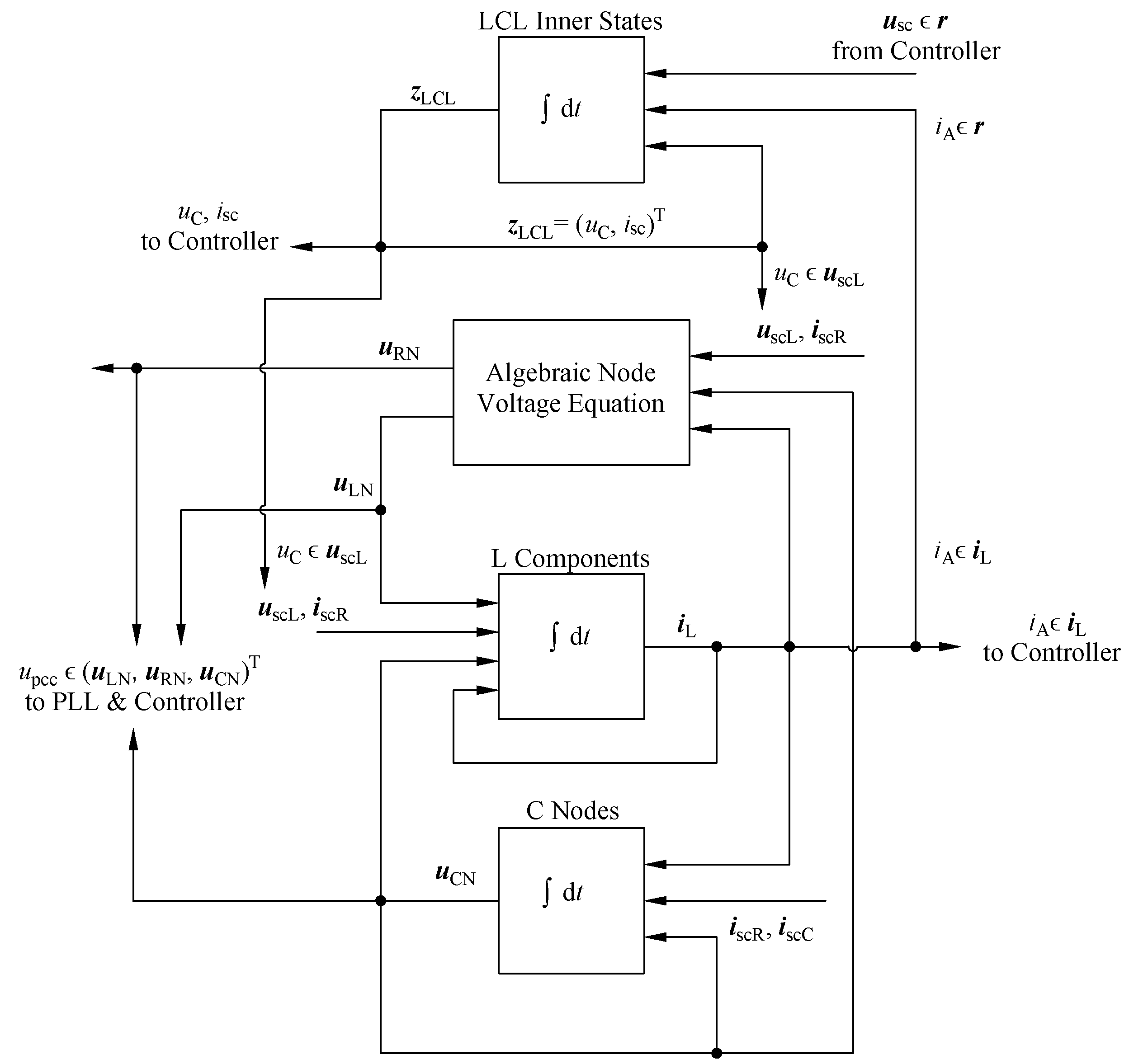
  • The inverter with the LCL filter is classified as an L component for the ENM. Its terminal current is part of the current vector  i L  and thus results directly from the DES in Equation (4). The parameters for the component matrices  R L  and  G L  are the grid-sided resistor  R f 2  and inductor  L f 2 .
  • As an L component, it is not decisive for the classification of the pcc node. The pcc node type depends on further connected component types. The terminal voltage can be either a result of the AES in Equation (3) ( u A u LN  or  u RN ) or of the DES in Equation (4) ( u A u CN ).
  • The LCL inverter has internal state variables to be considered in the IDES in Equation (5). These are the capacitor voltage  u C  and the source current  i sc , which are solved by the IDES in Equation (5). In order to avoid these internal variables, the model can also be broken down into its individual components, whereby the actual size of the DAE increases.
  • A cascaded control loop was developed for a grid-following inverter in the dq frame for decoupled active and reactive power control. An interface between the ENM network calculation results and the controller has been derived and displayed in detail. This framework is universally applicable for diverse inverter control approaches.
  • Different study cases were used to evaluate the ENM with grid-tied inverters, also with varying filter parameters, different load parameters, and node types of the pcc. The results show generally high accordance in comparison with the network calculation in Simulink. The differences between both tools were greatest for particularly weak networks. This approach is thus considered as validated to be further used for transient grid calculations.
As already mentioned, the inverter component presented here serves as a link to further preconnected DC/DC and DC applications, especially electrochemical components (cf. [46,47]). Regarding the power electronics part of the method, including the interaction of DC/DC and DC/AC applications, further validation with specially developed software will be useful. In the long term, the aim is to build a bridge to other energy carriers, so that gas and heating networks can be considered together with the electric power grid in a joint DAE to enable efficient coupled transient calculations for multi-energy grids. This point addresses integrated network planning interests as new configurations and system responses to transient switching actions can be quickly tested. In addition, combinations of the method with various optimization strategies (e.g., for maximum renewable feed-in or minimization of operating costs) for coupled grid operation are also conceivable.

Author Contributions

Conceptualization, D.V.; methodology, D.V.; software, D.V.; formal analysis, D.V.; writing—original draft preparation, D.V.; writing—review and editing, D.S.; visualization, D.V.; supervision, D.S.; project administration, D.S.; funding acquisition, Detlef Schulz. All authors have read and agreed to the published version of the manuscript.

Funding

This publication has been funded by the Open-Access-Publication-Fund of the Helmut Schmidt University/University of the Federal Armed Forces Hamburg and was developed during the project “Integrated network planning: Development of a network development planning methodology for the joint planning of the three energy sources electricity, gas and heat” funded by the Federal Ministry for Economic Affairs and Climate Action with the grant number 03EWR007H2.

Data Availability Statement

The data presented in this work are available on request from the corresponding author.

Acknowledgments

Thanks to Marc Schumann, Marc Florian Meyer, and Florian Grumm for professional dialogue and support during the writing of this paper.

Conflicts of Interest

The authors declare no conflicts of interest.

Abbreviations

The following abbreviations are used in this manuscript:
AESAlgebraic Equation System
AIArtificial Intelligence
ENMExtended Node Method
DAEDifferential-Algebraic-Equation-System
DESDifferential Equation System
IDESInner Differential Equation System
PLLPhase-Locked Loop

References

  1. Mahr, F.; Henninger, S.; Biller, M.; Jäger, J. Electrical Power Systems; Knowledge Networking of Converters, Grid Operation and Grid Protection; (Orig. German: Elektrische Energiesysteme; Wissensvernetzung von Stromrichter, Netzbetrieb und Netzschutz); Springer: Wiesbaden, Germany, 2021. [Google Scholar]
  2. Said-Romdhane, M.B.; Naouar, M.W.; Belkhodja, I.S.; Monmasson, E. An Improved LCL Filter Design in Order to Ensure Stability without Damping and Despite Large Grid Impedance Variations. Energies 2017, 10, 336. [Google Scholar] [CrossRef]
  3. Han, Y.; Yang, M.; Li, H.; Yang, P.; Xu, L.; Coelho, E.A.A. Modeling and Stability Analysis of LCL-Type Grid-Connected Inverters: A Comprehensive Overview. IEEE Access 2019, 7, 114975–115001. [Google Scholar] [CrossRef]
  4. Dursun, M.; Döşoğlu, M.K. LCL Filter Design for Grid Connected Three-Phase Inverter. In Proceedings of the 2018 2nd International Symposium on Multidisciplinary Studies and Innovative Technologies (ISMSIT), Ankara, Turkey, 19–21 October 2018; pp. 1–4. [Google Scholar] [CrossRef]
  5. Adamas-Pérez, H.; Ponce-Silva, M.; Mina-Antonio, J.D.; Claudio-Sánchez, A.; Rodríguez-Benítez, O.; Rodríguez-Benítez, O.M. A New LCL Filter Design Method for Single-Phase Photovoltaic Systems Connected to the Grid via Micro-Inverters. Technologies 2024, 12, 89. [Google Scholar] [CrossRef]
  6. Bolsi, P.C.; Prado, E.O.; Sartori, H.C.; Lenz, J.M.; Pinheiro, J.R. LCL Filter Parameter and Hardware Design Methodology for Minimum Volume Considering Capacitor Lifetimes. Energies 2022, 15, 4420. [Google Scholar] [CrossRef]
  7. Huang, L.; Wu, C.; Zhou, D.; Blaabjerg, F. Grid Impedance Impact on the Maximum Power Transfer Capability of Grid-Connected Inverter. In Proceedings of the 2021 IEEE 12th Energy Conversion Congress & Exposition—Asia (ECCE-Asia), Singapore, 24–27 May 2021; pp. 1487–1490. [Google Scholar] [CrossRef]
  8. Huang, L.; Wu, C.; Zhou, D.; Blaabjerg, F. Impact of Grid Strength and Impedance Characteristics on the Maximum Power Transfer Capability of Grid-Connected Inverters. Appl. Sci. 2021, 11, 4288. [Google Scholar] [CrossRef]
  9. Yazdani, A.; Iravani, R. Voltage-Sourced Converters in Power Systems; Modeling, Control and Applications; John Wiley & Sons, Inc.: Hoboken, NJ, USA, 2010. [Google Scholar]
  10. Fan, B.; Wang, X. Equivalent Circuit Model of Grid-Forming Converters with Circular Current Limiter for Transient Stability Analysis. IEEE Trans. Power Syst. 2022, 37, 3141–3144. [Google Scholar] [CrossRef]
  11. Gu, Y.; Bottrell, N.; Green, T.C. Reduced-order models for representing converters in power system studies. IEEE Trans. Power Electron. 2018, 33, 3644–3654. [Google Scholar] [CrossRef]
  12. Shah, C.; Vasquez-Plaza, J.D.; Campo-Ossa, D.D.; Patarroyo-Montenegro, J.F.; Guruwacharya, N.; Bhujel, N. Review of Dynamic and Transient Modeling of Power Electronic Converters for Converter Dominated Power Systems. IEEE Access 2021, 9, 82094–82117. [Google Scholar] [CrossRef]
  13. Paolone, M.; Gaunt, T.; Guillaud, X.; Liserre, M.; Meliopoulos, S.; Monti, A.; Van Cutsem, T.; Vittal, V.; Vournas, C. Fundamentals of power systems modelling in the presence of converter-interfaced generation. Electr. Power Syst. Res. 2020, 189, 106811. [Google Scholar] [CrossRef]
  14. Ajala, O.; Roberts, T.; Domínguez-García, A.D. Power-Flow Formulation for Inverter-Based Grids. In Proceedings of the 2023 IEEE Power & Energy Society General Meeting (PESGM), Orlando, FL, USA, 16–20 July 2023; pp. 1–5. [Google Scholar] [CrossRef]
  15. Bao, C.; Ruan, X.; Wang, X.; Li, W.; Pan, D.; Weng, K. Step-by-Step Controller Design for LCL-Type Grid-Connected Inverter with Capacitor–Current-Feedback Active-Damping. IEEE Trans. Power Electron. 2014, 29, 1239–1253. [Google Scholar] [CrossRef]
  16. Dmitruk, K. A Simplified Guide to Control Algorithms for Grid Converters in Renewable Energy Systems. Energies 2024, 17, 4690. [Google Scholar] [CrossRef]
  17. Yoon, S.-J.; Lai, N.B.; Kim, K.-H. A Systematic Controller Design for a Grid-Connected Inverter with LCL Filter Using a Discrete-Time Integral State Feedback Control and State Observer. Energies 2018, 11, 437. [Google Scholar] [CrossRef]
  18. Judewicz, M.G.; González, S.A.; Fischer, J.R.; Martínez, J.F.; Carrica, D.O. Inverter-Side Current Control of Grid-Connected Voltage Source Inverters with LCL Filter Based on Generalized Predictive Control. IEEE J. Emerg. Sel. Top. Power Electron. 2018, 6, 1732–1743. [Google Scholar] [CrossRef]
  19. Wang, X.; Wang, D.; Zhou, S. A Control Strategy of LCL-Type Grid-Connected Inverters for Improving the Stability and Harmonic Suppression Capability. Machines 2022, 10, 1027. [Google Scholar] [CrossRef]
  20. Park, K.S.; Seo, B.J.; Jo, K.R.; Heo, J.Y.; Kim, H.; Nho, E.C. Current Controller Design of a Grid Connected Inverter Using LCL Filter. In Proceedings of the 2019 10th International Conference on Power Electronics and ECCE Asia (ICPE 2019—ECCE Asia), Busan, Republic of Korea, 27–30 May 2019; pp. 2356–2361. [Google Scholar] [CrossRef]
  21. Kumari, K.; Jain, A.K. Cascaded control for LCL filter based grid-tied system with reduced sensors. IET Power Electron. 2022, 15, 1526–1539. [Google Scholar] [CrossRef]
  22. Huang, M.; Zhang, Z.; Wu, W.; Yao, Z. An Improved Three-Level Cascaded Control for LCL-Filtered Grid-Connected Inverter in Complex Grid Impedance Condition. IEEE Access 2022, 10, 65485–65495. [Google Scholar] [CrossRef]
  23. Xie, L.; Zeng, S.; Liu, J.; Zhang, Z.; Yao, J. Control and Stability Analysis of the LCL-Type Grid-Connected Converter without Phase-Locked Loop under Weak Grid Conditions. Electronics 2022, 11, 3322. [Google Scholar] [CrossRef]
  24. Lai, N.B.; Kim, K.H. Robust Control Scheme for Three-Phase Grid-Connected Inverters with LCL-Filter Under Unbalanced and Distorted Grid Conditions. IEEE Trans. Energy Convers. 2018, 33, 506–515. [Google Scholar] [CrossRef]
  25. Su, M.; Cheng, B.; Sun, Y.; Tang, Z.; Guo, B.; Yang, Y. Single-Sensor Control of LCL-Filtered Grid-Connected Inverters. IEEE Access 2019, 7, 38481–38494. [Google Scholar] [CrossRef]
  26. Gomes, C.C.; Cupertino, A.F.; Pereira, H.A. Damping techniques for grid-connected voltage source converters based on LCL filter: An overview. Renew. Sustain. Energy Rev. 2018, 81 Pt 1, 116–135. [Google Scholar] [CrossRef]
  27. Khan, D.; Zhu, K.; Hu, P.; Waseem, M.; Ahmed, E.M.; Lin, Z. Active damping of LCL-Filtered Grid-Connected inverter based on parallel feedforward compensation strategy. Ain Shams Eng. J. 2023, 14, 101902. [Google Scholar] [CrossRef]
  28. Gao, Y.; Wang, S.; Dragicevic, T.; Wheeler, P.; Zanchetta, P. Artificial Intelligence Techniques for Enhancing the Performance of Controllers in Power Converter-Based Systems—An Overview. IEEE Open J. Ind. Appl. 2023, 4, 366–375. [Google Scholar] [CrossRef]
  29. Fu, X.; Li, S. Control of Single-Phase Grid-Connected Converters with LCL Filters Using Recurrent Neural Network and Conventional Control Methods. IEEE Trans. Power Electron. 2016, 31, 5354–5364. [Google Scholar] [CrossRef]
  30. Uddin, M.N.; Tabrizi, Y.H. Artificial Intelligence Based Control Strategy of a Three-Phase Neutral-Point Clamped Back-to-Back Power Converter with Ensured Power Quality for WECS. In Proceedings of the 2022 IEEE Industry Applications Society Annual Meeting (IAS), Detroit, MI, USA, 9–14 October 2022; pp. 1–8. [Google Scholar] [CrossRef]
  31. Noura, H.N.; Allal, Z.; Salman, O.; Chahine, K. Explainable artificial intelligence of tree-based algorithms for fault detection and diagnosis in grid-connected photovoltaic systems. Eng. Appl. Artif. Intell. 2025, 139 Pt A, 109503. [Google Scholar] [CrossRef]
  32. Ramasubramanian, D.; Yu, Z.; Ayyanar, R.; Vittal, V.; Undrill, J. Converter model for representing converter interfaced generation in large scale grid simulations. IEEE Trans. Power Syst. 2017, 32, 765–773. [Google Scholar] [CrossRef]
  33. PLECS, The Simulation Platform for Power Electronic Systems. Available online: https://www.plexim.com/products/plecs (accessed on 7 January 2025).
  34. DIgSILENT | Power System Solutions, Powerfactory Applications. Available online: https://www.digsilent.de/en/powerfactory.html (accessed on 7 January 2025).
  35. Simulink, Simulink is for Model-Based Design. Available online: https://www.mathworks.com/products/simulink.html (accessed on 7 January 2025).
  36. Oswald, B.R. Three-Phase Grid Calculation; Calculation of Stationary and Transient Processes with Symmetrical Components and Space Phasors, 5th ed.; (orig. German: Berechnung von Drehstromnetzen; Berechnung stationärer und nichtstationärer Vorgänge mit Symmetrischen Komponenten und Raumzeigern); Springer: Wiesbaden, Germany, 2023. [Google Scholar]
  37. Hofmann, L. Efficient Calculation of Transients in Expanded Electrical Systems; (orig. German: Effiziente Berechnung von Ausgleichsvorgängen in ausgedehnten Elektroenergiesystemen); Shaker Verlag: Aachen, Germany, 2003. [Google Scholar]
  38. Oswald, B.R. Calculation of Transients in Electric Power Systems, Grid Calculation; (orig. German: Berechnung transienter Vorgänge in Elektroenergieversorgungsnetzen, Netzberechnung); VDE-Verlag: Berlin, Germany, 1996; Volume 2. [Google Scholar]
  39. Oswald, B.R. Computation of power systems transients by using sets of algebraic and of state space equations. In Proceedings of the International Conference on Power Systems Transients, Seattle, WA, USA, 22–26 June 1997; pp. 35–40. [Google Scholar]
  40. Oswald, B.R. Node-Oriented Methods of Grid Calculation, 2nd ed.; (orig. German: Knotenorientierte Verfahren der Netzberechnung); Leipziger University-Verlag: Leipzig, Germany, 2000. [Google Scholar]
  41. Oswald, B.R. Computation of Power Systems Eigenvalues Using the Modified Nodal Approach. Eur. Trans. Electr. Power 2000, 10, 7–12. [Google Scholar] [CrossRef]
  42. Hofmann, L. Extended Node Method: Separation of Slow and Dynamic Parts; (orig. German: Erweitertes Knotenpunktverfahren (EKPV): Entkopplung des langsamen vom dynamischen Teilsystem); Bericht IEE 629, Institut für Elektrische Energieversorgung, Universität Hannover: Hannover, Germany,, 2000. [Google Scholar]
  43. Hofmann, L.; Oswald, B. Efficient simulation of the dynamical behavior of large-scale power systems. Electr. Eng. 2001, 83, 307–311. [Google Scholar]
  44. Weidner, J. Contribution to Stationary and Transient Stability Analysis in Distribution Grids, (Orig. German: Beitrag zur statischen und transienten Stabilitätsanalyse in Verteilungsnetzen). Ph.D. Dissertation, Leibniz Universität Hannover, Hannover, Germany, 2021. [Google Scholar]
  45. Huisinga, H.; Hofmann, L. Analytical Properties of Differential-Algebraic Equations Arising in Circuit Simulation Using the Extended Nodal Approach, (orig. German: Strukturanalyse des mit dem Erweiterten Knotenpunktverfahren formulierten Differential-algebraischen Gleichungssystems). Automatisierungstechnik 2021, 69, 353–363. [Google Scholar] [CrossRef]
  46. Vorwerk, D.; Schumann, M.; Schulz, D. A Multi-Energy Fuel Cell Model in the Extended Node Method. In Proceedings of the NEIS 2023; Conference on Sustainable Energy Supply and Energy Storage Systems, Hamburg, Germany, 4–5 September 2023; pp. 245–254. [Google Scholar]
  47. Vorwerk, D.; Schumann, M.; Schulz, D. PEM-electrolyzer modelling and control strategies in the extended node method for hybrid power system modelling. In Proceedings of the 8th International Hybrid Power Plants & Systems Workshop (HYB 2024), Hybrid Conference, Azores, Portugal, 14–15 May 2024; pp. 385–392. [Google Scholar] [CrossRef]
  48. Vorwerk, D.; Schulz, D. Extended Node Method for Steady-State Heating Network Calculation based on Electric Analogies. In Proceedings of the 2023 11th International Conference on Smart Grid (icSmartGrid), Paris, France, 4–7 June 2023; pp. 1–8. [Google Scholar] [CrossRef]
  49. Maialen, B.; Thomas, J.-L. A review on synchronization methods for grid-connected three-phase VSC under unbalanced and distorted conditions. In Proceedings of the 2011 14th European Conference on Power Electronics and Applications, Birmingham, UK, 30 August–1 September 2011; pp. 1–10. [Google Scholar]
  50. MathWorks, Specialized Power Systems. Available online: https://de.mathworks.com/help/sps/specialized-power-systems.html (accessed on 24 October 2024).
  51. Simbench, Datasets. Available online: https://simbench.de/de/datensaetze/ (accessed on 24 October 2024).
Figure 1. Two-level three-phase grid-tied inverter with LCL filter configuration.
Energies 18 00344 g001
Figure 2. Single-phase electric circuit diagram of grid-tied inverter with LCL filter.
Energies 18 00344 g002
Figure 3. Single-phase electric circuit diagram of grid-tied inverter with LCL filter and parallel damping conductance.
Energies 18 00344 g003
Figure 4. Single-phase electric circuit diagram of grid-tied inverter with LCL filter and series damping resistor.
Energies 18 00344 g004
Figure 5. Cascaded grid current control loop for inverter with basic LCL filter in dq frame.
Energies 18 00344 g005
Figure 6. Synchronous reference frame phase-locked loop (PLL) for grid synchronization based on [49].
Energies 18 00344 g006
Figure 7. Combined grid calculation with the Extended Node Method and inverter control, basically taken from [36] and expanded with the LCL inner states and the interface with the cascaded current controller.
Energies 18 00344 g007
Figure 8. Bode plot of selected LCL filter design with exact values and  ± 20 % tolerance.
Energies 18 00344 g008
Figure 9. Single-phase electric circuit diagram for single grid-connected inverter with LCL filter.
Energies 18 00344 g009
Figure 10. System responses to sudden changes in active and reactive inverter power references  P *  and  Q *  with grid impedance  L g = 0.16  mH and  R g = 0.12 Ω : (a) Inverter terminal current  i A , abc . (b) Inverter terminal current and current references  I dq * . (c) PCC voltage  u abc  and  U dq . (d) Grid active and reactive power references  P *  and  Q *  and actual power P and Q.
Energies 18 00344 g010aEnergies 18 00344 g010b
Figure 11. System responses to sudden changes in active and reactive inverter power references  P *  and  Q *  with grid impedance  L g = 2  mH and  R g = 1.51 Ω : (a) Inverter terminal current  i A , abc . (b) Inverter terminal current and current references  I dq * . (c) PCC voltage  u abc  and  U dq . (d) Grid active and reactive power references  P *  and  Q *  and actual power P and Q.
Energies 18 00344 g011
Figure 12. System responses to sudden changes in active and reactive inverter power references  P *  and  Q *  with grid impedance  L g = 8  mH and  R g = 6.03 Ω : (a) Inverter terminal current  i A , abc . (b) Inverter terminal current and current references  I dq * . (c) PCC voltage  u abc  and  U dq . (d) Grid active and reactive power references  P *  and  Q *  and actual power P and Q.
Energies 18 00344 g012
Figure 13. System responses to sudden changes in active and reactive inverter power references  P *  and  Q *  with grid impedance  L g = 8  mH and  R g = 6.03 Ω  for varying filter parameters with  L ˜ f 1 = ζ L f 1 L ˜ f 2 = ζ L f 2 , and  C ˜ = ζ C : (a) Inverter terminal current  i A , c . (b) Inverter terminal currents  I d  and  I q . (c) Grid active and reactive power references  P *  and  Q *  and actual power P and Q.
Energies 18 00344 g013
Figure 14. Grid topology of sample network ’Simbench rural’ with connected inverters at nodes 5 and 9.
Energies 18 00344 g014
Figure 15. System responses to sudden changes in active and reactive inverter power references  P 1 * Q 1 *  and  P 2 * Q 2 *  in the Simbench rural testgrid for study case 1. (a) Inverter terminal currents  i A , abc . (b) Inverter terminal currents and current references  I dq * . (c) PCC voltages  u abc  and  U dq . (d) Grid active and reactive power references  P *  and  Q *  and actual power P and Q.
Energies 18 00344 g015aEnergies 18 00344 g015b
Figure 16. System responses to sudden changes in active and reactive inverter power references  P 1 * Q 1 *  and  P 2 * Q 2 *  in the Simbench rural testgrid for study case 1 (a) Inverter source currents  i sc , abc . (b) Inverter source currents  I sc , dq . (c) Capacitor voltage reference  U C , dq *  and actual voltage  U C , dq . (d) Inverter modulation signal  m dq .
Energies 18 00344 g016
Figure 17. System responses to sudden changes in active and reactive inverter power references  P 1 * Q 1 *  and  P 2 * Q 2 *  in the Simbench rural testgrid for study case 2. (a) Inverter terminal currents  i A , abc . (b) Inverter terminal currents and current references  I dq * . (c) PCC voltages  u abc  and  U dq . (d) Grid active and reactive power references  P *  and  Q *  and actual power P and Q.
Energies 18 00344 g017
Figure 18. System responses to sudden changes in active and reactive inverter power references  P 1 * Q 1 *  and  P 2 * Q 2 *  in the Simbench rural testgrid for study case 2. (a) Inverter source currents  i sc , abc . (b) Inverter source currents  I sc , dq . (c) Capacitor voltage reference  U C , dq *  and actual voltage  U C , dq . (d) Inverter modulation signal  m dq .
Energies 18 00344 g018
Table 1. Component types and their explicit state equations for the Extended Node Method [36].
Component TypeState Equation
L component   u L = L i ˙ L + R L i L + u q L
R component   i R = G R u R + i q R
C component   i C = C u ˙ C + G C u C + i q C
Table 2. Proposed LCL filter design and controller parameters.
ComponentParameter
Inverter with LCL Filter L f 1 = 2.0  mH,  R f 1 = 0.0163 Ω L f 2 = 1.4  mH,
R f 2 = 0.0109 Ω C = 0.6  µF,
U DC = 700  V,  f sw = 20  kHz
PLL K p = 0.02 K i = 0.1 ,
f pll = 20  kHz
Cascaded Controller K p , 1 = 5.6 K i , 1 = 43.6 K p , 2 = 0.08 ,
K i , 2 = 2.4 K p , 3 = 11.0 K i , 3 = 89.65 f ctrl = 20  kHz
Feed-Forward Compensation K = 1.0 τ = 0.00045  s
Table 3. Technical parameters for MV grid and MV/LV transformer in sample network.
ComponentParameter
MV Grid U n = 20  kV,  L g = 27.8723  mH,
R g = 0.8756 Ω ω 0 = 2 π · 50  rad/s
u sc , g , a ( t ) = 2 U n 3 cos ( ω 0 t )
Transformer U n , MV = 20  kV,  U n , LV = 400  V,  k = 50 ,
Type: Yy0,  L s = 0.119  mH,  R s = 0.008 Ω
Table 4. Load parameters for the LV Simbench Testgrid, regarding study cases 1 and 2.
LoadLoad Active and Reactive
Power Demand, Study
Case 1
Impedance Parameters,
Study Case 1
Load Active and Reactive
Power Demand, Study
Case 2
Impedance Parameters,
Study Case 2
Load 1 P load = 6  kW,  Q load = 2.37  kvar L load = 29.01  mH,  R load = 23.06 Ω P load = 12  kW,  Q load = 2  kvar C load = 39.79  µF,  G C , load = 0.075  S
Load 2 P load = 3  kW,  Q load = 1.19  kvar L load = 58.04  mH,  R load = 46.12 Ω P load = 6  kW,  Q load = 2.37  kvar L load = 29.02  mH,  R load = 23.06 Ω
Load 3 P load = 5  kW,  Q load = 1.97  kvar L load = 34.41  mH,  R load = 27.68 Ω P load = 10  kW,  Q load = 3.95  kvar L load = 17.41  mH,  R load = 13.84 Ω
Load 4 P load = 2  kW,  Q load = 0.79  kvar L load = 87.01  mH,  R load = 69.20 Ω P load = 4  kW,  Q load = 1.58  kvar L load = 43.51  mH,  R load = 34.60 Ω
Load 5 P load = 4  kW,  Q load = 1.58  kvar L load = 43.52  mH,  R load = 34.60 Ω P load = 8  kW,  Q load = 3.16  kvar L load = 21.76  mH,  R load = 17.3 Ω
Load 6 P load = 3  kW,  Q load = 1.19  kvar L load = 58.04  mH,  R load = 46.12 Ω P load = 6  kW,  Q load = 2  kvar C load = 39.79  µF,  G C , load = 0.0375  S
Load 7 P load = 8  kW,  Q load = 3.16  kvar L load = 21.76  mH,  R load = 17.30 Ω P load = 3.2  kW,  Q load = 1.27  kvar L load = 54.41  mH,  R load = 43.24 Ω
Load 8 P load = 14  kW,  Q load = 5.53  kvar L load = 12.434  mH,  R load = 9.88 Ω P load = 5.6  kW,  Q load = 2.21  kvar L load = 31.09  mH,  R load = 24.71 Ω
Load 9 P load = 3  kW,  Q load = 1.19  kvar L load = 58.04  mH,  R load = 46.12 Ω P load = 1.2  kW,  Q load = 0.47  kvar L load = 145.11  mH,  R load = 115.31 Ω
Load 10 P load = 12  kW,  Q load = 4.74  kvar L load = 14.50  mH,  R load = 11.53 Ω P load = 4.8  kW,  Q load = 1.90  kvar L load = 36.27  mH,  R load = 28.83 Ω
Load 11 P load = 2  kW,  Q load = 0.79  kvar L load = 87.01  mH,  R load = 69.20 Ω P load = 0.8  kW,  Q load = 0.32  kvar C load = 6.29  µF,  G C , load = 0.005 Ω
Load 12 P load = 4  kW,  Q load = 1.58  kvar L load = 43.52  mH,  R load = 34.60 Ω P load = 1.6  kW,  Q load = 0.63  kvar L load = 108.81  mH,  R load = 86.49 Ω
Load 13 P load = 14  kW,  Q load = 5.53  kvar L load = 12.43  mH,  R load = 9.88 Ω P load = 5.6  kW,  Q load = 2.21  kvar L load = 31.09  mH,  R load = 24.71 Ω
Disclaimer/Publisher’s Note: The statements, opinions and data contained in all publications are solely those of the individual author(s) and contributor(s) and not of MDPI and/or the editor(s). MDPI and/or the editor(s) disclaim responsibility for any injury to people or property resulting from any ideas, methods, instructions or products referred to in the content.

