Short-Term Load Forecasting in Power Systems Based on the Prophet–BO–XGBoost Model

Abstract

To tackle the challenges of limited accuracy and poor generalization in short-term load forecasting under complex nonlinear conditions, this study introduces a Prophet–BO–XGBoost-based forecasting framework. This approach employs the XGBoost model to interpret the nonlinear relationships between features and loads and integrates the Prophet model for label prediction from a time-series viewpoint. Given that hyperparameters substantially impact XGBoost’s performance, this study leverages Bayesian optimization (BO) to refine these parameters. Using a Gaussian process-based surrogate model and an acquisition function aimed at expected improvement, this framework optimizes hyperparameter settings to enhance model adaptability and precision. Through a regional case study, this method demonstrated improved predictive accuracy and operational efficiency, highlighting its advantages in both runtime and performance.

1. Introduction

With advancements in information technology and increasing reliance on renewable energy, short-term load forecasting has become essential for ensuring the reliable operation of the power grid [1]. In power systems, this process involves predicting electricity demand for upcoming days based on historical data and external influences [2]. Inputs typically include past load patterns, meteorological data, and calendar information, as well as real-time data such as weather forecasts. By analyzing the relationships between power demand and external factors, accurate predictions can be achieved for future intervals [3]. These forecasts play a key role in optimizing grid operations, reducing energy consumption, and improving economic efficiency [4].

The growing adoption of renewable energy, the advancement of smart grids, and climate change have introduced significant nonlinearity and time-varying characteristics to power loads, highlighting the need for enhanced accuracy and stability in short-term load forecasting [5]. Forecasting approaches are generally classified into two main types: conventional methods and machine learning-based methods. Traditional techniques include the ARMA model [6] and regression analysis [7]. Reference [8] proposed a seasonal autoregressive moving average (ARMA) model to analyze forecast errors in multivariate correlated loads, preserving key statistical properties of the data. Similarly, reference [9] presented a hybrid approach combining support vector regression and local prediction, demonstrating superior accuracy compared to conventional methods such as ARMA and artificial neural networks. While these methods are valued for their simplicity and computational efficiency, they require high data-sequence stationarity and are only effective in scenarios with minimal influencing factors. They struggle with abrupt load changes and have limited capacity to model nonlinear relationships [10]. As a result, their application is constrained when handling real-time system dynamics and fluctuations, and alternative approaches are needed to improve robustness.

With the rapid progress in artificial intelligence, machine learning has become a key tool in power load forecasting, greatly improving prediction accuracy. Algorithms such as decision trees [11], neural networks [12], and deep learning [13] are commonly utilized. The XGBoost algorithm, in particular, introduces a sparse-aware approach for parallel tree learning, enhancing training and prediction efficiency. It excels in handling large-scale, high-dimensional datasets [14]. Reference [15] developed an XGBoost model utilizing complete ensemble empirical mode decomposition with adaptive noise (CEEMDAN), which effectively captures error sequence fluctuations. This model integrates well with various load prediction frameworks, delivering robust and precise forecasting. Reference [16] combined clustering techniques with the XGBoost algorithm for short-term load prediction. By employing the K-means algorithm for classification and constructing XGBoost regression models tailored to each category, this method provides accurate load estimates. Reference [17] introduced an approach based on ISFS and XGBoost, which leverages the improved spanning-tree forward selection (ISFS) algorithm for feature selection. The XGBoost model assesses features through cross-validation, enhancing training performance and reducing prediction errors. Furthermore, reference [18] proposed a hybrid model integrating LightGBM and XGBoost that was specifically designed to handle multi-feature data selection and error correction efficiently, meeting the rigorous demands of short-term electricity load forecasting.

In machine learning research, parameter tuning is critical for enhancing model accuracy. Manual tuning, however, often introduces variability, limiting the potential of the XGBoost algorithm [19]. Integrating optimization algorithms with machine learning offers a solution by leveraging optimization techniques for parameter selection, thus enhancing model performance in specific scenarios. Reference [20] applied the sparrow search algorithm, utilizing its multi-objective optimization capability to fine-tune XGBoost parameters and achieving higher prediction accuracy. Similarly, reference [21] employed the fireworks algorithm, which mimics the behavior of explosions to efficiently search a solution space. It demonstrated effectiveness in solving complex optimization challenges. Reference [22] adopted Bayesian optimization (BO) to fine-tune hyperparameters, offering high search efficiency and global optimization capabilities. Lastly, reference [23] compared a grid search with cross-validation and BO for hyperparameter tuning, showing that BO-based XGBoost delivers superior accuracy and efficiency compared to a grid search.

This study integrates traditional forecasting techniques with machine learning to propose a Prophet–BO–XGBoost-based method for short-term load forecasting in complex nonlinear environments. The key contributions of this research include the following:

(1) Using the XGBoost model to explore the relationships between feature values and load while leveraging the Prophet model for time series-based label prediction.

(2) Employing the BO algorithm to optimize XGBoost hyperparameters, with the Gaussian process as the surrogate model and the expected improvement as the acquisition function, ensuring optimal parameter selection and enhanced predictive performance under diverse conditions.

This method leverages the strengths of time-series trend modeling and the ability of machine learning algorithms to capture nonlinear features, addressing the challenges of forecasting in complex nonlinear environments. The main contributions of this study are as follows:

(1) A hybrid forecasting framework combining the Prophet and XGBoost models: This framework fully exploits the advantages of the Prophet model in trend and seasonality modeling for time series and the XGBoost model’s capacity to capture complex nonlinear relationships. By integrating these two approaches, the proposed framework not only enhances the model’s understanding of the global trends in load characteristics but also significantly improves forecasting accuracy under complex conditions.

(2) Bayesian optimization for efficient hyperparameter tuning and performance enhancement: Bayesian optimization employs Gaussian processes to model the objective function and uses an expected improvement strategy to efficiently search for optimal hyperparameter combinations. Compared with traditional methods, this optimization strategy adapts more effectively to diverse load scenarios, further enhancing the model’s predictive performance and generalization capability.

The structure of this paper is as follows: Section 1 introduces the Prophet time-series model. Section 2 examines the XGBoost machine learning model’s principles. Section 3 proposes the Prophet–BO–XGBoost-based short-term load forecasting method. Section 4 validates this method using load data from a specific region. Section 5 presents this study’s conclusions.

2. Prophet Time-Series Forecasting Model

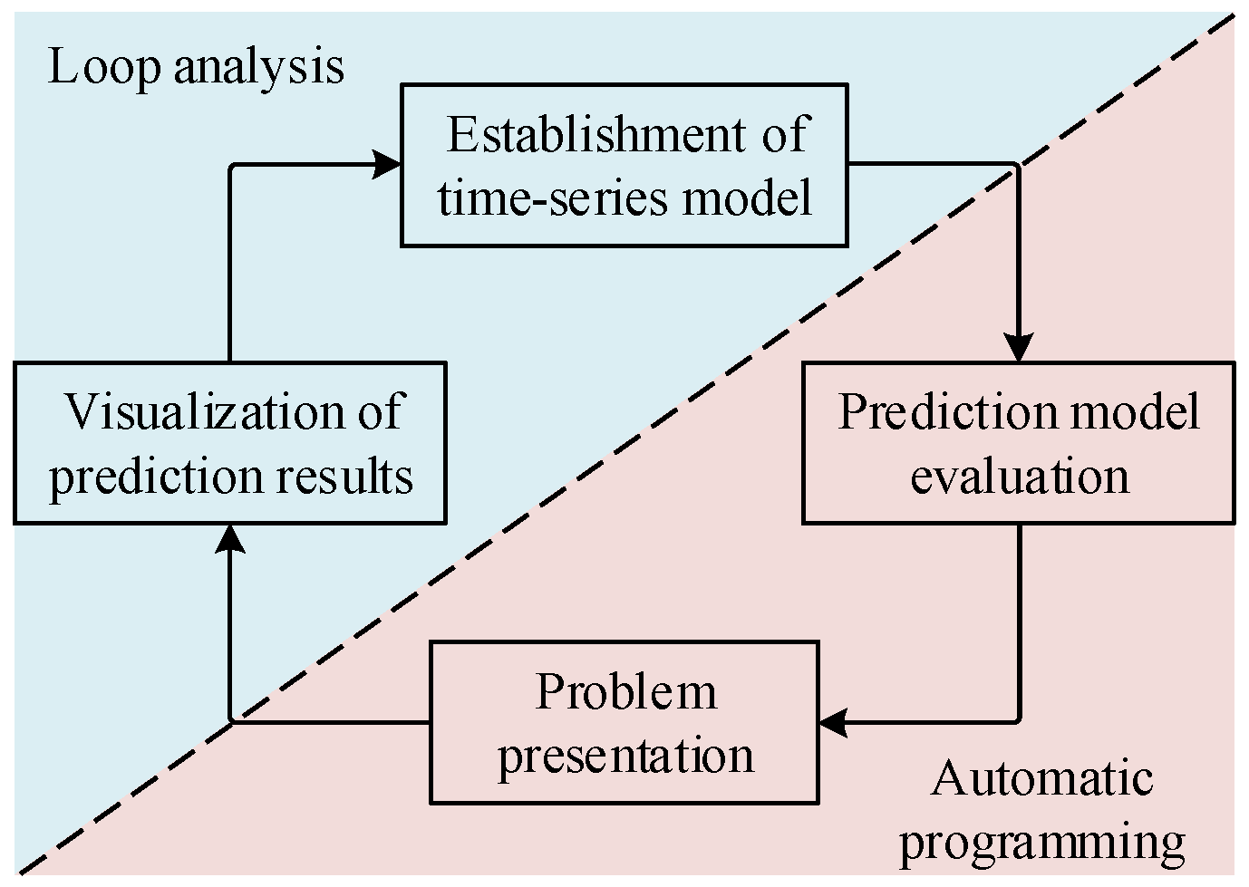
The Prophet model integrates two main modules (modeling and evaluation), as illustrated in Figure 1. The basic process of the Prophet model involves establishing a time-series model based on the forecasting problem, continuously evaluating the model to adjust its parameters, and ultimately providing feedback on all prediction results through visualization.

Prophet is a time-series prediction model that incorporates three core components: trend (g(t)), seasonality (s(t)), and holidays (h(t)). These components are combined mathematically as follows:

$$P(t)=g(t)+s(t)+h(t)+{\epsilon }_t$$

(1)

where ε_t is the error component, which is typically assumed to follow a normal distribution with a mean of 0. It is used to reflect unexpected variations that are not accounted for in the model.

The trend component (g(t)) is used to capture the long-term trend in the time series. Its fundamental form is

$$g(t)=(k+\alpha {(t)}^T\delta )t+(b+\alpha {(t)}^T\gamma )$$

(2)

where k is the growth rate; b is the bias parameter; δ is the change in the growth rate; γ is the adjustment value process offset at points where the growth rate (k) changes; and α(t)^T indicates whether a slope or offset adjustment is performed (1 for yes or 0 for no).

The seasonal component (s(t)) is approximated using a Fourier series to represent periodic variations. It is expressed as follows:

$$s(t)={\displaystyle \sum _{n=1}^N(a_n\cos (\frac{2\pi nt}{P})+b_n\sin (\frac{2\pi nt}{P}))}$$

(3)

where N is the total number of periods; P denotes a specific fixed period; 2n is the expected number of occurrences in this period in the model; and a_n and b_n are parameters that need to be estimated.

The holiday component (h(t)) is used to consider abnormal data fluctuations occurring on specific dates that cannot be captured by periodic models. Therefore, independent models are established for different holidays. Its specific form is as follows:

$$h(t)=Z(t)\kappa$$

(4)

$$Z(t)=[I(t\in D_1),I(t\in D_2),\cdots ,I(t\in D_L)]$$

(5)

$$\kappa \in \mathrm{Normal}(0,v^2)$$

(6)

where D_i represents the i-th holiday set; I(t ∈ D_i) is the indicator function, which has a value of 1 during the i-th holiday period and a value of 0 otherwise; κ is the holiday setting parameter; and v is the impact factor of holidays on the prediction results, where a larger v implies that holiday has a greater influence.

3. XGBoost Machine Learning Model

The XGBoost model improves upon the gradient-boosting algorithm by integrating multiple base classifiers (decision trees), significantly enhancing classification and prediction performance. Figure 2 illustrates the overall workflow of the XGBoost model. Initially, the training data are used to construct an initial decision tree, which provides a preliminary prediction of the target variable and generates the first-round results. In each subsequent iteration, the model calculates the residuals between the current predictions and the actual values, and these residuals are fed into the next decision tree. The new tree is guided to learn and correct the deficiencies of the previous predictions. Each new decision tree aims to minimize the current errors, allowing the model to iteratively optimize the predictions. Once all decision trees are trained, their outputs are combined using a weighted aggregation mechanism to produce the final ensemble result. Through this iterative optimization process, XGBoost effectively approximates the true target values, delivering highly efficient and accurate predictions.

The XGBoost algorithm employs decision trees as base learners to construct multiple weak learners. It then continuously trains the model in the direction of gradient descent. Assuming the model consists of k decision trees, the formulation is as follows:

$${\widehat{y}}_i={\displaystyle \sum _{i=1}^k{f}_t(x_i),f_t\in F}$$

(7)

$$F=\{f_t(x_i)={\omega }_{q(x_i)}\}$$

(8)

where k is the number of trees; f_t denotes the function in function space F; ${\widehat{y}}_i$ is the predicted value of the model; x_i is the input of the i-th data point; ${\omega }_{q(x_i)}$ denotes the weight of the leaf node where sample x_i occurs; and q(x_i) indicates the leaf node corresponding to sample x_i.

The XGBoost algorithm adopts an addition and forward distribution algorithm, where each iteration does not affect the original model, that is

$$\left\{\begin{array}{l}{\widehat{y}}_i^{(0)}=0\\ {\widehat{y}}_i^{(1)}={\widehat{y}}_i^{(0)}+f_1(x_i)\\ ⋮\\ {\widehat{y}}_i^{(t)}={\widehat{y}}_i^{(t-1)}+f_t(x_i)\end{array}\right.$$

(9)

The XGBoost algorithm’s objective function (L) consists of two components: the loss function, which quantifies the error between the predicted and actual loads in the test dataset, and the regularization term, which mitigates overfitting and manages model complexity. The mathematical representation of the objective function is

$$L={\displaystyle \sum _{i=1}^{n}l(y_i,{\widehat{y}}_i)}+{\displaystyle \sum _{j=1}^k\mathsf{\Omega }(f_j)}$$

(10)

$$\mathsf{\Omega }(f)=\gamma T+{\displaystyle \frac{1}{2}}\lambda \left|\right|\omega |{|}^2$$

(11)

where $l(y_i,{\widehat{y}}_i)$ represents the error between the predicted and actual values; Ω(f_j) is the regularization term used to reduce overfitting; T denotes the number of leaf nodes; γ is the penalty factor for T; w indicates the weights of the leaf nodes; and n is the sample size. Upon training the t-th tree, the objective function is revised as

$$L^{(t)}={\displaystyle \sum _{i=1}^{n}l(y_i,{\widehat{y}}_i)}+{\displaystyle \sum _{j=1}^t\mathsf{\Omega }(f_j)}={\displaystyle \sum _{i=1}^{n}l(y_i,{\widehat{y}}_i)}+{\displaystyle \sum _{j=1}^{t-1}\mathsf{\Omega }(f_j)}+\mathsf{\Omega }(f_t)$$

(12)

Since the previous t−1 regression trees are known information, i.e., Ω(f_j) is constant, the optimization process for the t-th tree is unaffected. Therefore, the objective function can be simplified to

$$L^{(t)}={\displaystyle \sum _{i=1}^{n}l(y_i,{\widehat{y}}_i)}+\mathsf{\Omega }(f_t)={\displaystyle \sum _{i=1}^{n}l(y_i,{\widehat{y}}_i)}+\gamma T+{\displaystyle \frac{1}{2}}\lambda \left|\right|\omega |{|}^2$$

(13)

The objective function can be rewritten in terms of leaf node traversal as

$$L^{(t)}=\gamma T+{\displaystyle \sum _{j=1}^T({\displaystyle \sum _{i\in I_j}l(y_i,{\widehat{y}}_i)}+\frac{1}{2}\lambda {\omega }_j^2)}=\gamma T+{\displaystyle \sum _{j=1}^T({\displaystyle \sum _{i\in I_j}l(y_i,{\widehat{y}}_i^{(t-1)}+{\omega }_j)}+\frac{1}{2}\lambda {\omega }_j^2)}$$

(14)

By expanding the objective function using the Taylor series for a binary function, $l(y_i,{\widehat{y}}_i^{(t-1)}+{\omega }_j)$ can be represented as

$$l(y_i,{\widehat{y}}_i^{(t-1)}+{\omega }_j)=l(y_i,{\widehat{y}}_i^{(t-1)})+l^{\prime }(y_i,{\widehat{y}}_i^{(t-1)}){\omega }_j+{\displaystyle \frac{1}{2}}{l}^{″}(y_i,{\widehat{y}}_i^{(t-1)}){\omega }_j^2$$

(15)

When the objective function is simplified by removing the term $l(y_i,{\widehat{y}}_i^{(t-1)})$, the following equation is obtained:

$$\tilde{L}(t)=\gamma T+{\displaystyle \sum _{j=1}^T({\displaystyle \sum _{i\in I_j}(h_i{\omega }_j+\frac{1}{2}{g}_i{\omega }_j^2})+\frac{1}{2}\lambda {\omega }_j^2)}=\gamma T+{\displaystyle \sum _{j=1}^T({\omega }_j{\displaystyle \sum _{i\in I_j}{h}_i+}\frac{1}{2}{\omega }_j^2(\lambda +{\displaystyle \sum _{i\in I_j}{g}_i}))}$$

(16)

where $h_i=l^{\prime }(y_i,{\widehat{y}}_i^{(t-1)})$ and $g_i=l^{″}(y_i,{\widehat{y}}_i^{(t-1)})$.

A lower value for the objective function reflects a more optimal regression tree structure. Minimizing it and setting its derivative to zero yields the weights for each leaf node as follows:

$${\omega }_j=-{\displaystyle \frac{{\displaystyle \sum _{i=I_j}{h}_i}}{{\displaystyle \sum _{i=I_j}{g}_i+\lambda }}}$$

(17)

By substituting them into the objective function, the minimum loss ($\tilde{L}(t)$) at this point is

$${\tilde{L}}^t(q)=-{\displaystyle \frac{1}{2}}{\displaystyle \sum _{j=1}^T\frac{({\displaystyle \sum _{i\in I_j}{h}_i})}{{\displaystyle \sum _{i\in I_j}{g}_i+\lambda }}}+\gamma T$$

(18)

The construction of the XGBoost prediction model involves the following steps: (1) start with an initial iteration, building sub-models sequentially; (2) before each iteration, compute the first-order g_i and second-order h_i derivatives of the loss function for all training samples; (3) generate a new decision tree and calculate the predicted values for each leaf node using Equation (17); and (4) incrementally add the newly generated model to the existing models after each iteration, forming the final prediction model over multiple iterations.

4. Prophet–BO–XGBoost Load Forecasting Model

4.1. Bayesian Optimization of XGBoost Hyperparameter Tuning

The XGBoost model’s hyperparameters include general, booster, and task parameters, with the booster parameters being the most influential. For instance, the learning rate (η) updates the leaf node weights, where a small η can cause overfitting and a large η may lead to underfitting. Thus, optimizing XGBoost hyperparameters is essential for enhancing model performance.

In general, hyperparameters can be determined using grid search or random search methods. However, these approaches involve significant randomness and chance and may not fully exploit the performance of the XGBoost algorithm. To address this issue, this study adopts the BO algorithm to optimize the XGBoost machine learning model. By leveraging previous evaluation information, BO reduces the number of attempts required to find the optimal hyperparameters.

The BO algorithm involves constructing a surrogate probability model for the loss function and iteratively refining it with new information to approximate the true distribution. The hyperparameter optimization of the XGBoost model using this algorithm is formulated as follows:

$$x^{*}=\arg \max f(x_i)x_i\in {ℝ}^{\mathrm{d}}$$

(19)

where x_i indicates the XGBoost model’s hyperparameters; f(·) represents the objective function assessing model performance; ℝ is the hyperparameter space; and d denotes the dimensionality of the hyperparameters to be optimized. The optimal hyperparameters are represented as x*. The evaluation results of XGBoost are recorded as y_i = f(x_i).

Bayesian optimization relies on two key components: the surrogate model and the acquisition function. The surrogate model estimates the objective function’s value and facilitates optimization of black-box functions. The acquisition function selects the next sampling point, balancing exploration and exploitation to improve the objective function value in subsequent steps. This study utilizes a Gaussian process (g(x)) as the surrogate model and adopts expected improvement (α(x|D)) as the acquisition function.

4.1.1. Gaussian Process (GP)

The Gaussian process approximates an objective function by defining a probability distribution for each of its points. It models a series of random vectors that evolve over time, where all sub-vectors follow a Gaussian distribution at any given time. A stochastic process {X_t, t∈T} is Gaussian if, for any finite index set (T and t₁…t_k∈T), the random vector X_t1…tk = (X_t1,…,X_tk) is multivariate and normal. This implies that any linear combination of X_t1 to X_tk is normally distributed.

Denoting the Gaussian process as GP(·), which is characterized by a mean function (m) and a covariance function (k), its mathematical representation is

$$f(x)~\mathrm{GP}(m(x),k(x,x\prime ))$$

(20)

where k(·) denotes the covariance function, defined as

$$k(x_i,x_j)=\exp (-{\displaystyle \frac{1}{2}}{‖x_i-x_j‖}^2)$$

(21)

Let D_1:t = {x_1:t, f_1:t} represent historical data from exploration. Assuming the next search value is x_t+1 and f_t+1 = f(x_t+1), the covariance matrix is denoted as K:

$$\mathit{K}=\left[\begin{array}{ccc}k(x_1,x_1)& \cdots & k(x_1,x_t)\\ ⋮& \ddots & ⋮\\ k(x_t,x_1)& \cdots & k(x_t,x_t)\end{array}\right]$$

(22)

According to the properties of Gaussian processes, f_1:t and f_t+1 constitute a joint Gaussian distribution, assuming a mean of zero. This distribution is expressed as

$$\left[\begin{array}{l}{f}_{1:t}\\ f_{t+1}\end{array}\right]~N\left(0,\left[\begin{array}{cc}\mathit{K}& \mathit{k}\\ {\mathit{k}}^T& k(x_{t+1},x_{t+1})\end{array}\right]\right)$$

(23)

$$\mathit{k}=[\begin{array}{cccc}k(x_{t+1},x_1)& (x_{t+1},x_2)& \dots & (x_{t+1},x_i)\end{array}]$$

(24)

By finding its marginal density function, the result can be obtained as

$$f_{t+1}|D_{1:t},x_{t+1}~N({\mu }_t(x_{t+1}),{\sigma }_t^2(x_{t+1}))$$

(25)

$${\mu }_t(x_{t+1})={\mathit{k}}^T{\mathit{K}}^{-1}{f}_{1:t}$$

(26)

$${\sigma }_t^2(x_{t+1})=k(x_{t+1},x_{t+1})-{\mathit{k}}^T{\mathit{K}}^{-1}\mathit{k}$$

(27)

Based on the above analysis, the normal distribution followed by x_t+1 at any given value can be estimated, thereby allowing for the setting of a specific objective function to locate the optimal x_t+1 for the next step.

4.1.2. Expected Improvement (EI)

The expected improvement criterion seeks to find the x_t+1 that maximizes the expected improvement while balancing exploration and exploitation. Once an x_t+1 is chosen, the optimization function is expressed as

$$I(x)=\max \{0,f_{t+1}(x)-f(x^{+})\}$$

(28)

where x⁺ denotes the current best sample. The desired x_t+1 should satisfy

$$x=\arg \max \mathbb{Z}(\max \{0,f_{t+1}(x)-f(x^{+})\left\}\right|D_t)$$

(29)

The formula for the expected improvement can be reformulated as follows:

$$\mathbb{Z}(I)=\sigma (x)\left[{\displaystyle \frac{\mu (x)-f(x^{+})}{\sigma (x)}}\mathsf{\Phi }\left({\displaystyle \frac{\mu (x)-f(x^{+})}{\sigma (x)}}\right)+\varphi \left({\displaystyle \frac{\mu (x)-f(x^{+})}{\sigma (x)}}\right)\right]$$

(30)

The final simplified result is

$$\mathrm{EI}(x)=\left\{\begin{array}{ll}(\mu (x)-f(x^{+}))\mathsf{\Phi }(Z)+\sigma (x)\varphi (Z)\hfill & \sigma (x)>0\hfill \\ 0\hfill & \sigma (x)=0\hfill \end{array}\right.$$

(31)

where $Z={\displaystyle \frac{\mu (x)-f(x^{+})}{\sigma (x)}}$, ϕ(·) represents the standard normal probability density function, and F(·) denotes its cumulative distribution function.

The Bayesian optimization algorithm employs Bayes’ theorem to guide the search for the objective function’s maximum value. At each iteration, it uses historical observation data to refine the optimization process, aiming to identify the best hyperparameter combination. The optimization framework is detailed in

Table 1. The workflow of the Bayesian optimization framework.

Bayesian Optimization Framework
Input:	Initial point count (n0); maximum iterations (N); surrogate model (g(x)); acquisition function (α(x|D)).
Start
Step 1:	Randomly generate n0 initial points (Xinit = {x0, x1,…, xn0−1}).
Step 2:	Compute their function values (f(Xinit)) and form the initial dataset (D0 = {Xinit, f(Xinit)}). Set t = n0 and Dt−1 = D0.
while t < N
Step 3:	Build the surrogate model (g(x)) using the current dataset (Dt−1).
Step 4:	Optimize the acquisition function (α(x|Dt−1)) to determine the next evaluation point: xt = argmin α(x|Dt−1).
Step 5:	Evaluate f(xt) at xt and update the dataset (Dt = Dt−1$\cup${xt, f(xt)}), then return to step 3.
end while
Output:	Optimal evaluation point.
End

, while Figure 3 illustrates the BO–XGBoost model’s process, with the steps described as follows:

(1) Data preprocessing: The input data are first standardized and normalized to eliminate discrepancies in feature scales, ensuring the consistency and quality of the input data. The processed data are then divided into training and testing sets, which are used for model training and performance evaluation, respectively.

(2) Initial sampling and model updating for Bayesian optimization: Bayesian optimization begins by randomly sampling from the hyperparameter space to construct a surrogate model using a Gaussian process. Through iterative updates, the surrogate model gradually fits the objective function distribution, enhancing the efficiency and accuracy of the sampling process.

(3) Hyperparameter optimization and optimal configuration: In each iteration, the expected improvement strategy is used to select new sampling points, calculate objective function values (e.g., prediction errors), and evaluate whether the optimization goal has been achieved. Once the goal has been met, the optimal hyperparameter configuration for the XGBoost model is output.

(4) BO–XGBoost model training: Using the optimal hyperparameters obtained through Bayesian optimization, the XGBoost model is trained. The model iteratively constructs multiple decision trees, correcting prediction errors step by step. The final predictions are generated by aggregating the outputs of all decision trees with weighted combinations, achieving high-precision predictions of the target variable.

(5) Model evaluation: after training, the testing set is fed into the model to assess its performance using evaluation metrics, validating the accuracy of the predictions.

4.2. Hybrid Prediction Model

According to the power load data, we construct both the Prophet model and the XGBoost machine learning model. Let us assume that at time t the forecasted value from the Prophet model is denoted as P(t) and the forecasted value from the BO–XGBoost machine learning model is denoted as X(t), where t = 1, 2, …n. Then, we combine these two individual models into an integrated Prophet–BO–XGBoost hybrid prediction model. This model can be defined as follows:

$$Y_t={\omega }_{1}P(t)+{\omega }_{2}X(t)$$

(32)

$${\omega }_1={\displaystyle \frac{{\epsilon }_X}{{\epsilon }_P+{\epsilon }_X}}$$

(33)

$${\omega }_2={\displaystyle \frac{{\epsilon }_P}{{\epsilon }_P+{\epsilon }_X}}$$

(34)

where ε_P and ε_X represent the average relative errors of Prophet and XGBoost, respectively, and Y_t denotes the mixed forecast value at time t.

The reciprocal error method, as shown in Equations (33) and (34), is applied to determine the weights. This method assigns larger weights to models with smaller average relative errors, aiming to reduce the overall average relative error of the mixed model and obtain more accurate forecast values.

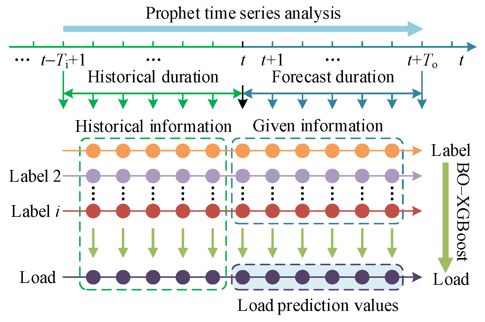
Figure 4 illustrates the load prediction model based on Prophet–BO–XGBoost. The Prophet model predicts labels from a time-series perspective, represented by the horizontal arrows, which indicate the analysis along the time axis. Conversely, the vertical arrows represent the BO–XGBoost analysis, which captures the nonlinear relationships between multiple labels and the power load. Bayesian optimization fine-tunes the XGBoost model’s hyperparameters, while the BO–XGBoost model captures the nonlinear relationships between features and power load, enabling horizontal short-term load forecasting. The detailed model construction steps are outlined below:

(1) Collect relevant data, including historical load data and corresponding raw feature data, and preprocess the data samples for labeling.

(2) Establish the Prophet model to forecast various labels and obtain components such as trend, weekly, and yearly data.

(3) Utilize the Prophet results as feature variables. Maintain consistency in the number of training and testing sample sets with the Prophet model. Establish the Prophet–XGBoost optimization model using the training sample set. Optimize the hyperparameters using Bayesian optimization, analyzing the nonlinear mapping relationships between various labeled feature values and the load.

(4) Output the prediction results and calculate the accuracy.

5. Case Analysis

To assess this model’s accuracy and performance, the mean absolute percentage error (δ_MAPE) and root-mean-square error (δ_RMSE) were chosen as evaluation metrics [24]:

$${\delta }_{MAPE}={\displaystyle \frac{({\displaystyle \sum _{i=1}^n\left|\frac{{\widehat{y}}_i-y_i}{y_i}\right|})}{n}}\times 100\%$$

(35)

$${\delta }_{RMSE}=\sqrt{{\displaystyle \frac{1}{n}}{\displaystyle \sum _{i=1}^n{({\widehat{y}}_i-y_i)}^2}}$$

(36)

where y_i represents the actual observed load value at time point i; ${\widehat{y}}_i$ represents the predicted load value at the same time point generated by the BO–XGBoost model; and n denotes the total number of data samples, i.e., the number of time points.

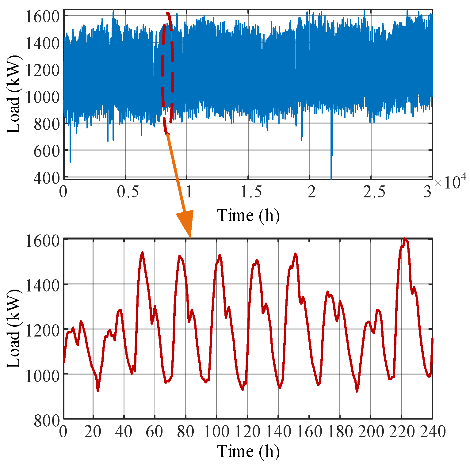
Load data from 2018 to 2020 for a specific region, along with features like temperature and humidity, were used as training and testing datasets. Figure 5 illustrates the load dataset.

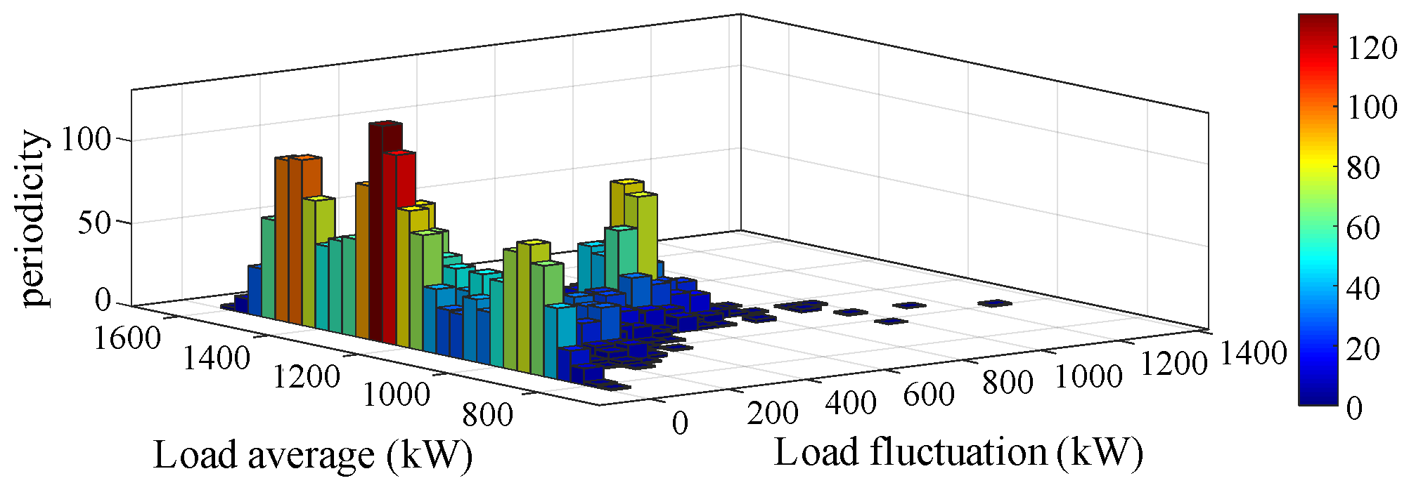
The rainflow counting technique was used for statistical analysis of the load in this area, as depicted in Figure 6. The analysis revealed that the load predominantly ranged between 800 kW and 1400 kW, with most fluctuations measuring between 200 kW and 400 kW.

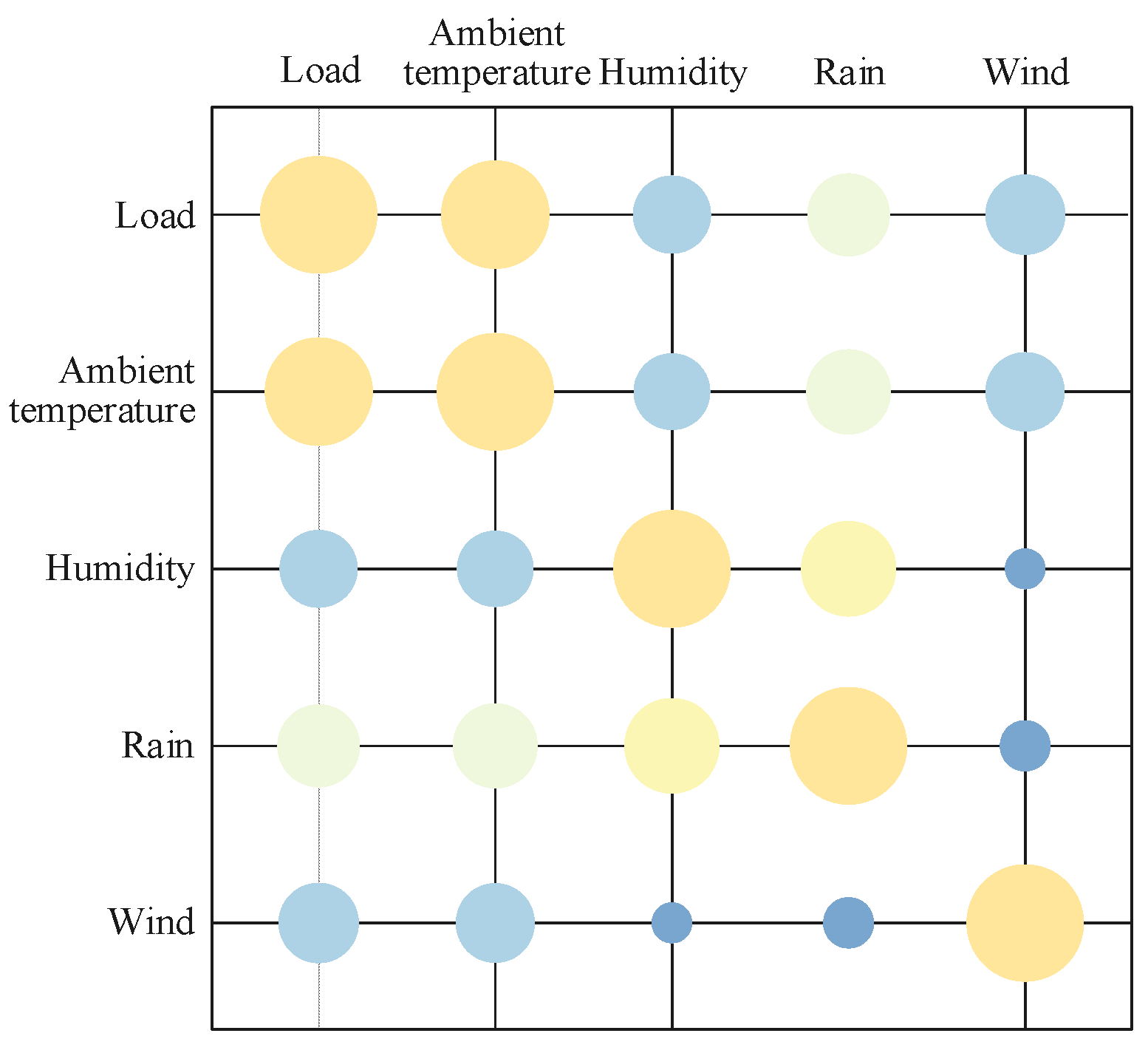
The regional load level was closely related to environmental variables such as temperature, humidity, precipitation, and wind speed. To ensure the scientific validity and rationality of the selected input features, Pearson correlation analysis was conducted to quantify the relationships between the load and key environmental variables, particularly temperature and humidity. The results, as shown in Figure 7, indicate significant correlations between the load and these variables, with temperature and humidity exerting strong influences on load variations. In the figure, the size of the circles represents the strength of the correlations, with larger circles indicating stronger correlations. This analysis not only validates the relevance and rationality of the selected features but also ensures a close association between the input features and the target load, providing a reliable data foundation for subsequent modeling.

In the Anaconda environment, a 10-fold cross-validation method was applied, using the RMSE as the target for Bayesian optimization. This approach identified the best hyperparameters for the XGBoost model, as shown in

Table 2. The optimal hyperparameters for the XGBoost model.

XGBoost Hyperparameter	Optimal Value
max_depth	9
learning_rate	0.042
n_estimators	810
min_child_weight	19.653
subsample	0.808
colsample	0.428
reg_alpha	17.384
gamma	0.079

.

Figure 8 illustrates 48 h load predictions made using decision trees, random forests, XGBoost, and the proposed Prophet–BO–XGBoost algorithm. The results indicate that the predicted load generated by the proposed method aligns closely with the actual load.

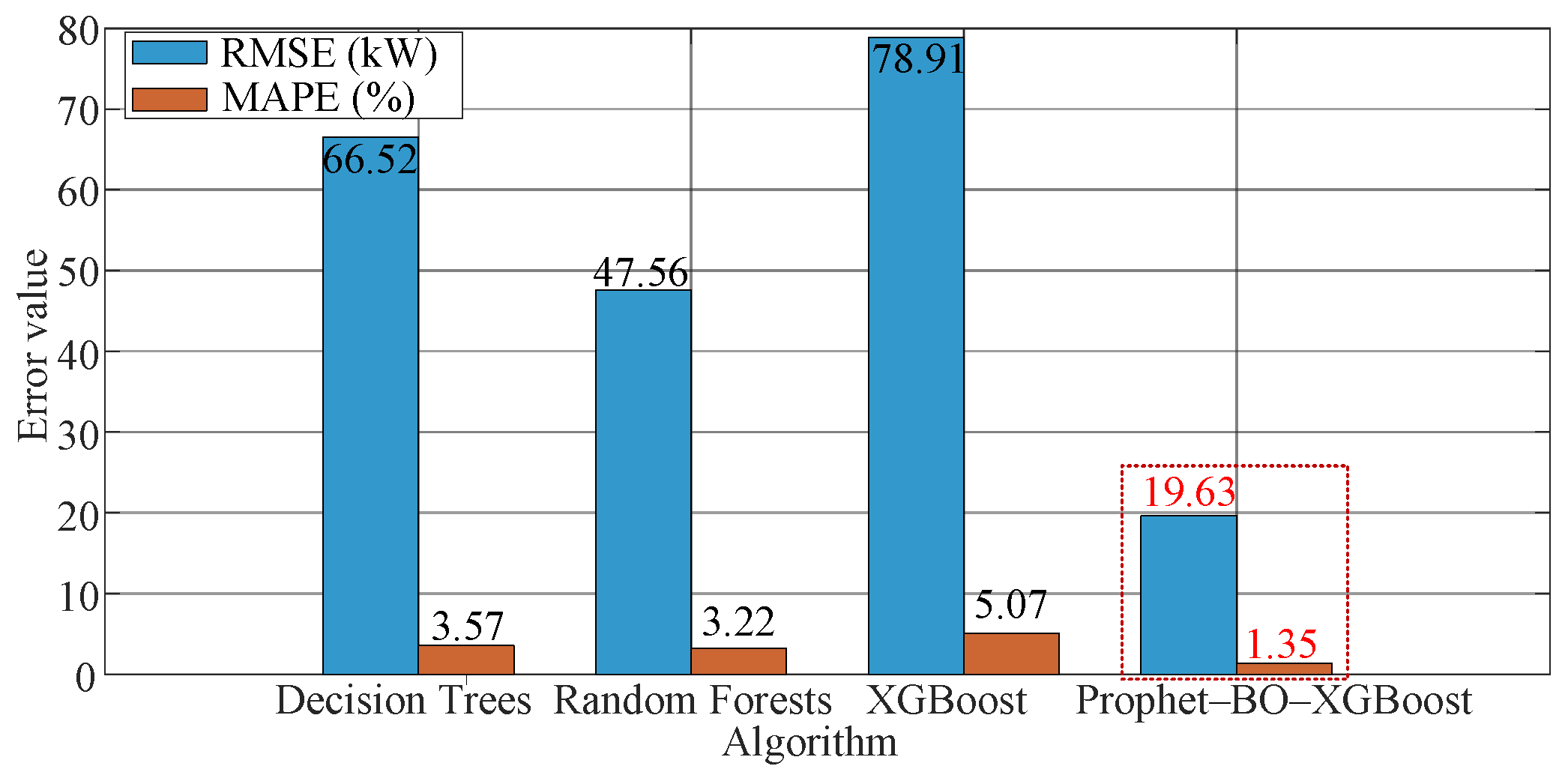
Figure 9 illustrates the predictive errors (measured by the RMSE and MAPE) of four algorithms: decision trees, random forests, XGBoost, and the proposed Prophet–BO–XGBoost. The results clearly demonstrate the superior performance of the Prophet–BO–XGBoost algorithm, which achieved the lowest error values for both metrics (RMSE: 19.63 kW, MAPE: 1.35%). In comparison, the other algorithms showed higher error levels, indicating limitations in error control. These findings highlight the exceptional predictive accuracy of the proposed algorithm and provide a reference for selecting and optimizing forecasting models in future studies.

Table 3. Prediction errors of various algorithms.

Algorithm	RMSE (kW)	MAPE (%)
decision trees	66.517	3.567
random forests	47.556	3.223
XGBoost	78.910	5.071
Prophet–BO–XGBoost	19.629	1.352

presents the RMSE and MAE values of 48 h load predictions made using decision trees, random forests, XGBoost, and the Prophet–BO–XGBoost algorithm. The results indicate that the proposed method achieved the lowest RMSE and MAE, demonstrating superior predictive performance.

6. Conclusions

The Prophet–BO–XGBoost-based method for short-term load forecasting effectively tackles the issues of low accuracy and poor generalization in complex nonlinear scenarios. The case study analysis led to the following conclusions:

(1) The hybrid model presented integrates the Prophet model with the XGBoost machine learning algorithm, leveraging their complementary strengths. The case studies demonstrated that this combined approach enhances the accuracy of short-term load forecasting, offering an effective solution for addressing complex nonlinear scenarios.

(2) The Prophet–XGBoost algorithm comprehensively evaluates the impacts of variables like temperature, humidity, and wind speed, effectively mitigating overfitting. It facilitates feature selection, boosts prediction accuracy, and enhances the interpretability of the regression model.

(3) Compared to conventional hyperparameter tuning techniques, the XGBoost model employing Bayesian optimization demonstrates superior efficiency in exploring its hyperparameters. It dynamically adjusts the balance between exploration and exploitation processes, facilitating the discovery of the global optimal solution. Consequently, this approach significantly improves the model’s performance and its ability to generalize across different datasets.

(4) The BO–XGBoost model proposed in this study demonstrates strong performance in short-term load forecasting. However, its predictive accuracy is highly sensitive to the initial feature selection, as the rationality of feature selection directly impacts the model’s performance. Future research could explore automated feature selection methods, leveraging feature importance analysis techniques such as SHAP values, to further optimize feature engineering and reduce the impact of manual intervention on model performance.