SA-STGCN: A Spectral-Attentive Spatio-Temporal Graph Convolutional Network for Wind Power Forecasting with Wavelet-Enhanced Multi-Scale Learning

Abstract

Wind power forecasting remains a major challenge for renewable energy integration, as conventional models often perform poorly when confronted with complex atmospheric dynamics. This study addresses the problem by developing a Spectral-Attentive Spatio-Temporal Graph Convolutional Network (SA-STGCN) designed to capture the intricate temporal and spatial dependencies of wind systems. The approach first applies wavelet transform decomposition to separate volatile wind signals into distinct frequency components, enabling more interpretable representation of rapidly changing conditions. A dynamic temporal attention mechanism is then employed to adaptively identify historical patterns that are most relevant for prediction, moving beyond the fixed temporal windows used in many existing methods. In addition, spectral graph convolution is conducted in the frequency domain to capture farm-wide spatial correlations, thereby modeling long-range atmospheric interactions that conventional localized methods overlook. Although this design increases computational complexity, it proves critical for representing wind variability. Evaluation on real-world datasets demonstrates that SA-STGCN achieves substantial accuracy improvements, with a mean absolute error of 1.52 and a root mean square error of 2.31. These results suggest that embracing more expressive architectures can yield reliable forecasting performance, supporting the stable integration of wind power into modern energy systems.

1. Introduction

As global reliance on finite resources like oil and natural gas becomes increasingly untenable, the transition to renewable energy has emerged as an irreversible global trend [1]. The wind power sector, in particular, has demonstrated exceptional growth. According to the Global Wind Report 2025 by the Global Wind Energy Council (GWEC), 2024 marked another record year with 117 GW of new wind capacity installed worldwide, bringing the total cumulative capacity to 1136 GW. Onshore wind continues to be the backbone of this expansion, reaching a cumulative capacity of 1052.3 GW and accounting for approximately 92.7% of the total global installations by the end of 2024 [2]. The large-scale integration of wind power, which is essential for achieving carbon neutrality, is fundamentally constrained by its inherent intermittency and stochastic characteristics. The output from a wind farm is highly sensitive to a variety of complex and dynamic factors, including not only meteorological variables but also the geographical topology of the turbines [3]. This unpredictability introduces significant risks to power system operations, complicating grid dispatch and jeopardizing system reliability. To address these challenges and fully harness the potential of wind energy, it is therefore crucial to develop accurate and robust power forecasting technologies [4,5].

The development of wind power prediction methods reflects an evolutionary shift from physical and statistical models to advanced machine learning and deep learning approaches, driven by the continuous pursuit of higher prediction accuracy and advancements in computational science. In the early stages, wind power forecasting primarily relied on two categories of models. The first category consisted of physical models based on numerical weather prediction (NWP), which employed the control equations of fluid mechanics and atmospheric science to simulate atmospheric conditions. These models are grounded in rigorous theoretical principles and exhibit low dependency on historical data [6]. However, their high computational demands constrain frequent model updates, making it difficult to meet the real-time requirements of short-term forecasting. The second category encompassed traditional statistical models, such as autoregressive moving average (ARMA) [7] and autoregressive integrated moving average (ARIMA) [8]. These models demonstrated high computational efficiency by capturing linear patterns in historical observations. However, their predictive robustness diminished when confronted with the strong nonlinearity and non-stationary fluctuations inherent in wind speed data.

With the rapid advancement of computing power, machine learning has emerged as an effective tool for addressing the nonlinear challenges in wind power prediction. Traditional machine learning techniques, including support vector machines (SVM) [9], (Categorical Boosting) Catboost [10], and random forests (RF) [11], have shown strong capabilities in modeling nonlinear patterns. Nevertheless, the performance of these models heavily depends on the quality of feature engineering. If critical physical or statistical patterns are not effectively extracted and represented as input features, the generalization ability of the model may be significantly compromised. The emergence of deep learning (DL) marked a paradigm shift in this domain [12]. Unlike conventional approaches that rely on manual feature engineering, deep learning models can automatically learn complex nonlinear mappings from raw data in an end-to-end manner, directly linking meteorological inputs with power outputs. Consequently, current research has increasingly focused on sophisticated architectures capable of capturing multi-variable interactions and spatiotemporal dependencies to enhance prediction accuracy [13].

The application of deep learning in wind power forecasting initially centered on classical models such as long short-term memory networks (LSTM) and convolutional neural networks (CNN), which were employed to extract temporal dynamics and local spatial features, respectively. To better capture spatial correlations among wind turbines, graph neural networks (GNNs) have emerged as a key technological breakthrough, as demonstrated by Peng et al. [14]. Researchers have moved beyond static, geography-based graph structures and explored multi-graph construction methods that integrate multi-dimensional information, as shown by Zhao et al. [15], These approaches are often combined with reinforcement learning for dynamic model integration, as explored by Yu et al. and Zhao et al. [15,16]. Additionally, attention mechanisms are increasingly used to interpret model decision-making processes, as implemented by Zhang et al. [17]. And dynamic graph techniques capable of adaptively learning graph structures, developed by Xie et al. [18].

In recent years, research has increasingly emphasized practical application scenarios. To address the “black box” nature of deep learning models, explainability analysis has gained prominence. In time series feature extraction, more advanced architectures such as the Transformer have been introduced, and even dual-domain Transformers capable of joint time-frequency analysis have been developed to uncover deeper dynamic patterns, as proposed by Hou et al. [19]. Considering the economic implications of prediction errors in electricity markets, researchers have proposed asymmetric loss functions tailored to decision costs, as developed by Liang et al. and Dong et al. [20,21], and have developed online learning frameworks coupled with concept drift detection mechanisms to adapt to evolving data distributions, as presented by He et al. [22]. Furthermore, a growing trend involves shifting from deterministic point predictions to probabilistic interval predictions, offering richer information for grid risk management, as demonstrated by Li et al. [23]. Cutting-edge research now integrates multiple components into unified frameworks, such as deep fusion of historical power data and environmental variables using novel architectures like Kolmogorov-Arnold networks (KANs), as developed by Wu et al. [24], or combining signal processing techniques (e.g., VMD, MODWT) for multi-scale data preprocessing and analysis, as shown by Qiao et al. and Gao et al. [25,26], leading to end-to-end predictive systems.

Recently, significant progress has been made in enhancing wind power forecasting through graph neural networks (GNNs), focusing on optimizing graph construction, improving physical interpretability, addressing scalability challenges, and quantifying prediction uncertainty. In terms of model fusion and integration, Qu et al. proposed a dual-stacking ensemble spatiotemporal graph deep neural network based on multiple ensemble strategies. This model integrates Bagging, LSTM, and RF through a sophisticated stacking algorithm to fully exploit the spatiotemporal correlations within wind farm clusters, achieving high-precision multi-step-ahead forecasting [27]. To enhance physical realism, Qiu et al. incorporated turbine-level “blocking effects” into their spatiotemporal GNN to better simulate airflow interactions [28]. For large-scale deployment, Wang et al. designed a comprehensive framework from data preprocessing to prediction, employing an improved DBSCAN algorithm for anomaly detection and repair, and using spectral clustering to partition wind farms into sub-clusters for parallel prediction, thereby improving computational efficiency and scalability [29]. To quantify prediction uncertainty, Liao et al. combined GNNs with an enhanced Bootstrap technique to achieve ultra-short-term probabilistic interval forecasting, providing valuable support for risk-informed decision-making in power systems [30]. Qu et al. integrated prediction intervals with expert behaviors into a deep reinforcement learning framework to enhance the economic operation of microgrids. This approach effectively mitigates prediction uncertainty and improves training efficiency, leading to more robust and cost-effective power scheduling decisions [31].

In summary, wind power forecasting research has now entered a stage of deeper integration and more refined modeling. Although existing models have made progress in capturing both spatial and temporal patterns, they continue to face challenges in handling the complex dynamics of wind energy systems. In particular, current methods struggle to represent the different time scales of variability, to adaptively pinpoint which past conditions are most relevant, and to capture the large-scale, non-local spatial correlations driven by broader meteorological systems. These unresolved challenges remain key obstacles to further improving forecasting accuracy and form the central motivation of this study.

To address these challenges, we propose the Spectral-Attentive Spatio-Temporal Graph Convolutional Network (SA-STGCN). Our model uses a unified framework—not because such a framework is inherently superior, but because it provides the right foundation to combine three complementary components that directly target the above problems. The power of SA-STGCN lies in how these elements work together. The process starts by transforming the raw and unstable wind power time series with a wavelet transform. This step decomposes the noisy signal into different frequency sub-bands, making the data easier to interpret. In doing so, it separates long-term, relatively stable wind patterns from short-term, turbulent fluctuations. This multi-scale representation then serves as the input for the predictive core of the model. Inside this block, a Temporal Attention mechanism scans the historical sequence and highlights the most influential past time steps. This allows the network to focus on key precursors—such as those leading up to sudden output ramps. At the same time, the model handles spatial relationships by moving beyond the limitations of conventional localized graph message passing. Instead, it adopts Spectral Graph Convolution, which operates in the graph’s spectral space to extract global, farm-level correlations influenced by large weather systems. By combining multi-resolution decomposition, adaptive temporal weighting, and global spatial filtering, SA-STGCN builds a richer representation of wind dynamics than conventional models can achieve.

We tested SA-STGCN using a real-world dataset collected from a wind farm in central China. Experimental results show that our model delivers significantly better forecasting performance than current state-of-the-art (SOTA) methods. To summarize, the main contributions of this paper are:

(1)

We propose SA-STGCN, a new unified spatiotemporal framework that improves the STGCN architecture for accurate short-term wind power forecasting. Its integration of frequency analysis, temporal attention, and spectral graph theory enables stronger and more coherent modeling of the coupled spatial and temporal characteristics of wind power.

(2)

The model introduces a tri-fold innovation. First, a wavelet transform is applied as a front-end feature extraction tool, breaking the time series into multiple frequency bands to reveal both short- and long-term patterns. Second, a Temporal Attention mechanism embedded in each block adaptively identifies the most relevant historical time steps, solving the problem of static temporal kernels. Third, the use of Spectral Graph Convolution, based on the graph Laplacian, enables the model to capture global and multi-scale spatial connections—going beyond the limits of purely local graph operations.

(3)

Through comprehensive evaluation on the collected dataset, we show that SA-STGCN achieves significantly better forecasting accuracy than existing SOTA methods, proving its effectiveness for modeling complex spatiotemporal systems.

The rest of this paper is organized as follows. Section 2 explains the SA-STGCN architecture and methodology. Section 3 describes the dataset, preprocessing steps, and evaluation metrics. Section 4 presents the experimental setup, model performance, and comparison with other baselines. Finally, Section 5 concludes with key findings and discusses future research directions.

2. Materials and Methods

2.1. Problem Description

The spatiotemporal forecasting problem in wind farm power generation aims to predict future power outputs by leveraging historical data, while explicitly modeling the spatial dependencies among turbines within the farm. Concretely, given historical observations of length $l$, the objective is to generate forecasts for the subsequent $O$ time steps, with emphasis typically placed on short-term prediction scenarios:

$${\hat{Y}}_{k+1:k+O}=f(Y_{k-l+1:k},A)$$

(1)

where $Y_{k-l+1:k}$ denotes the observed historical time series from time $k-l+1$ to $k$, ${\hat{Y}}_{k+1:k+O}$ is the predicted future time series from time $k+1$ to $k+O$, and $A$ encapsulates the spatial dependencies among turbines and meteorological stations within the wind farm. The function $f(·)$ represents the predictive model employed.

The SA-STGCN architecture, illustrated in Figure 1, comprises three integrated stages that process dual-stream inputs through sophisticated spatiotemporal modeling to generate wind power forecasts. The framework initiates with concurrent processing of turbine SCADA data and gridded meteorological data, where each input time series undergoes multi-resolution feature extraction equivalent to wavelet transform, decomposing signals into frequency sub-bands that capture features across different time scales. These enhanced features are projected through a Graph Embedding Layer into high-dimensional latent space, creating a unified spatiotemporal graph tensor with dimensions (Batch, Channels, Nodes, Time) that integrates turbine and weather data into a structured representation. The core processing occurs through multiple stacked SA-STGCN blocks that iteratively refine spatiotemporal representations, with each block processing input tensor X_in through a sequence of operations including Temporal Attention for dynamic feature importance computation across time dimensions, Gated Temporal Convolution for local sequential pattern capture, Spectral Graph Convolution operating in the graph’s frequency domain to model complex non-local spatial dependencies, and additional Gated Temporal Convolution for further feature processing, all stabilized through residual connections and Layer Normalization to enable deep architecture training. The final prediction stage employs a Select & Aggregate operation to isolate turbine node features while discarding auxiliary weather nodes, followed by aggregation of selected turbine features to produce unified wind farm representation, Feature Flattening to create a single vector, and processing through an Output MLP Head that maps learned spatiotemporal features to a predicted power output for the desired forecast horizon.

2.2. Graph Construction from Geospatial Data

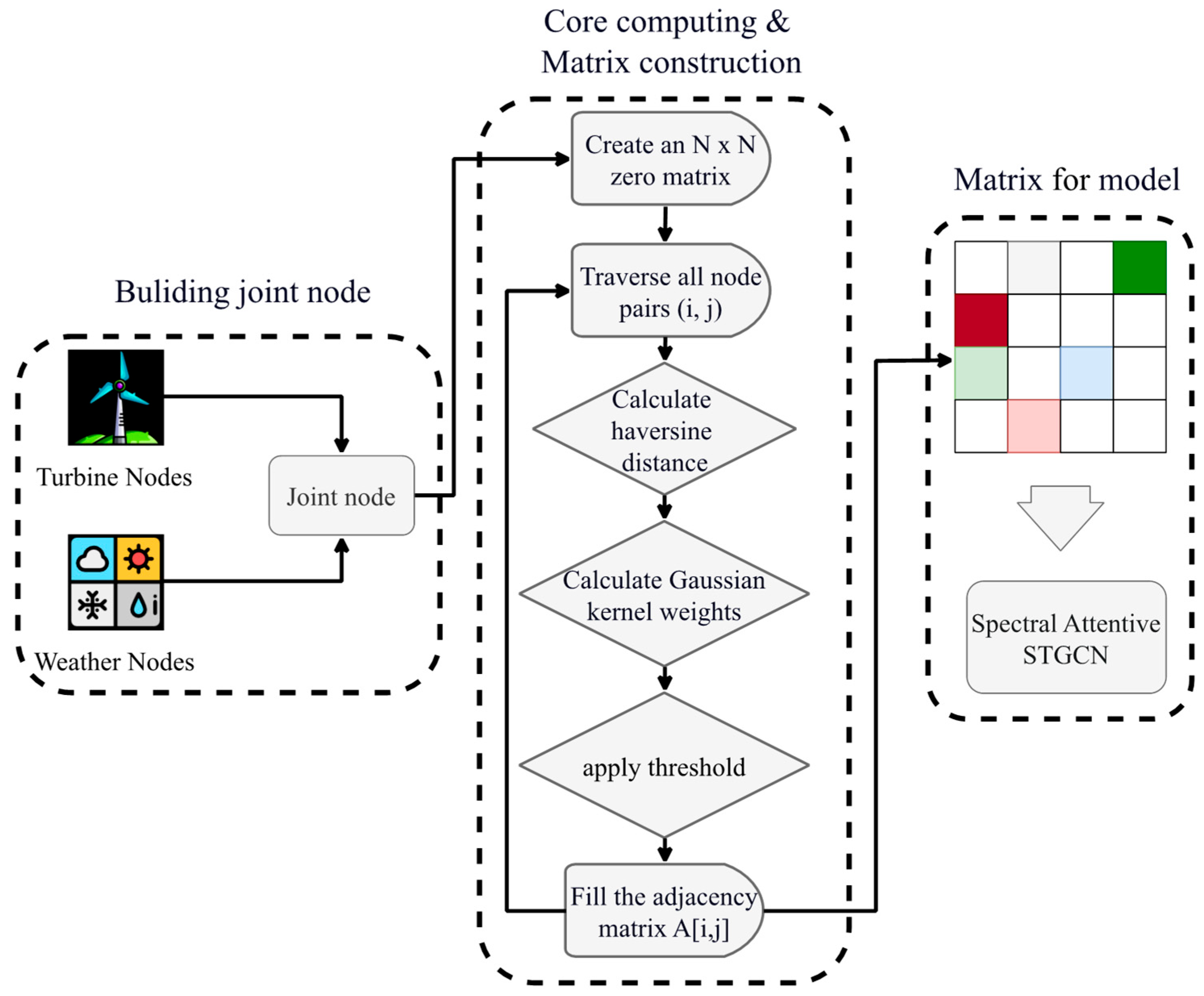
The foundation of our spatiotemporal model is a graph structure that effectively represents the physical relationships between wind turbines and surrounding meteorological points. We define a graph $G=(V,E,A)$, where $V$ is the set of nodes, $E$ is the set of edges, and $A\in {ℝ}^{N\times N}$ is the weighted adjacency matrix. The process of constructing this graph is illustrated in Figure 2.

We create a unified set of joint nodes by combining the $N_t$ turbine nodes with the $N_w$ meteorological grid nodes, resulting in a total of $N=N_t+N_w$ nodes. Each node is characterized by its geographical coordinates. The adjacency matrix $A$ is then constructed based on the principle that closer nodes should have a stronger connection. For every pair of nodes $(i,j)$ in the graph, the geographical separation is first measured using the Haversine distance, denoted as $d(i,j)$. This distance is then transformed into a similarity weight using a Gaussian kernel function, ensuring that the weight decays exponentially as the distance increases. The weight $A_{ij}$ is calculated as:

$$A_{ij}=exp(-{\displaystyle \frac{d{(i,j)}^2}{{\sigma }^2}})$$

(2)

where $\sigma$ is a hyperparameter that controls the width of the kernel, dictating the scale of spatial influence. To create a sparse and meaningful graph structure while removing weak or irrelevant connections, a threshold $\epsilon$ is applied to the calculated weights. Any weight below this threshold is set to zero. The resulting matrix $A$, which encodes the weighted spatial topology of the entire system, serves as the fundamental input for the subsequent layers of our Spectral Attentive STGCN.

Figure 1. The architecture of the for SA-STGCN short-term wind power forecasting.

Figure 1. The architecture of the for SA-STGCN short-term wind power forecasting.

Figure 2. The flowchart for constructing the weighted adjacency matrix.

Figure 2. The flowchart for constructing the weighted adjacency matrix.

2.3. Input & Multi-Resolution Feature Extraction

With the graph structure established, the next stage involves preparing the input features for each node. The raw time-series data, while informative, often contains complex patterns operating at different frequencies. To enable the model to capture both short-term fluctuations and long-term trends, we employ a multi-resolution feature extraction module based on the Discrete wavelet transform (DWT).

The DWT decomposes a time-series signal into a set of wavelet coefficients, which include a low-frequency approximation component and several high-frequency detail components. This process effectively separates the signal based on its frequency content. For a given input feature time-series $x(t)$ from either a turbine or a weather node, the DWT produces a set of sub-series:

$$x(t)\stackrel{DWT}{\to }\{c{A}_k(t),c{D}_k(t),c{D}_{k-1}(t),\dots ,c{D}_1(t)\}$$

(3)

where $c{A}_k$ is the approximation coefficients at level $k$, and $c{D}_i$ is the detail coefficients at levels $i=1,\dots ,k$. These decomposed sub-series, representing different frequency bands of the original signal, are concatenated along the feature dimension. This concatenation significantly enriches the feature representation for each node, providing the model with a more comprehensive, multi-scale view of the input data. Subsequently, the raw static features are integrated with the enhanced time-series representations. This unified feature set is then mapped into a high-dimensional latent space through dedicated embedding layers, enabling a comprehensive representation that captures both temporal dynamics and spatial characteristics. T his results in the initial spatiotemporal graph tensor $X_0\in {ℝ}^{B\times C\times N\times T_{in}}$, which serves as the input to the first SA-STGCN block.

2.4. Temporal Attention Module

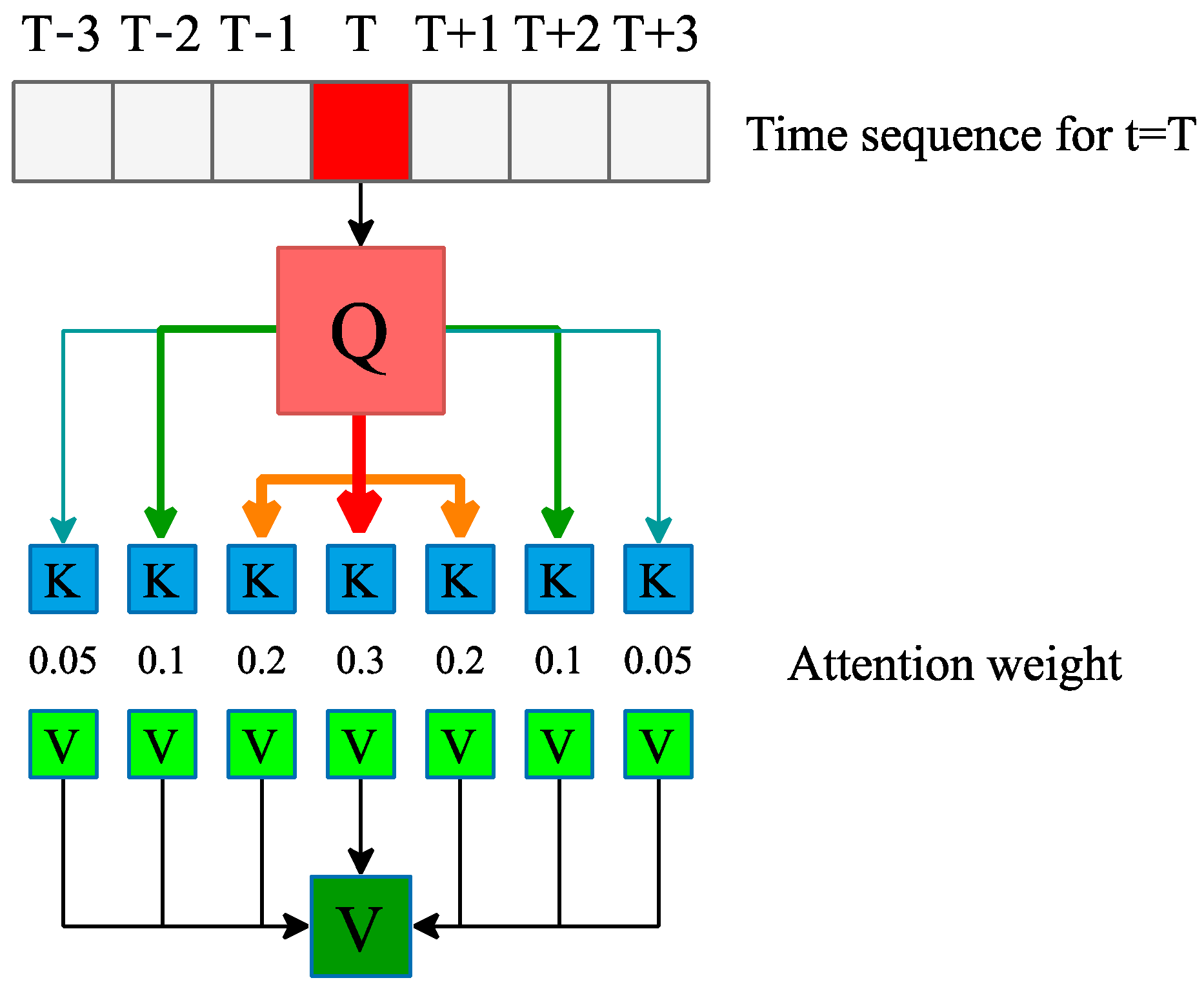
To capture long-range dependencies and dynamically identify the most salient time steps, each SA-STGCN block incorporates a Temporal Attention module. This module allows the model to assign different importance weights to different points in the input time series, rather than treating them equally. The underlying mechanism is the scaled dot-product attention, as illustrated in Figure 3.

Given an input tensor $X\in {ℝ}^{B\times C\times N\times T}$, we first treat the temporal dimension as the sequence to which attention is applied. The input features for each node are projected into three distinct matrices: the Query ($Q$), key ($K$), and Value ($V$) matrices, using a shared linear projection layer:

$$Q,K,V=X{W}_Q,X{W}_K,X{W}_V$$

(4)

where $W_Q,W_K,W_V\in {ℝ}^{C\times C}$ are learnable weight matrices. The attention scores are then computed by taking the dot product of the Query with the Key, which measures the similarity or relevance between each pair of time steps. To prevent the dot product values from growing too large and causing vanishing gradients in the softmax function, the scores are scaled by the square root of the head dimension, $d_k$. The attention weights are subsequently obtained by applying a softmax function along the key dimension. Finally, the output of the attention layer is a weighted sum of the Value vectors, where the weights are the computed attention scores. The full operation is defined as:

$$Attention(Q,K,V)=softmax({\displaystyle \frac{Q{K}^T}{\sqrt{d_k}}})V$$

(5)

In our multi-head attention implementation, this process is performed in parallel for $h$ heads, each operating on a different subspace of the features. The outputs of all heads are then concatenated and linearly projected to produce the final output of the module. This multi-head mechanism allows the model to jointly attend to information from different representation subspaces at different positions. The output of the temporal attention module is then added to the original input via a residual connection to preserve the original information while incorporating temporal dependencies.

2.5. Spatial Modeling: Spectral Graph Convolution

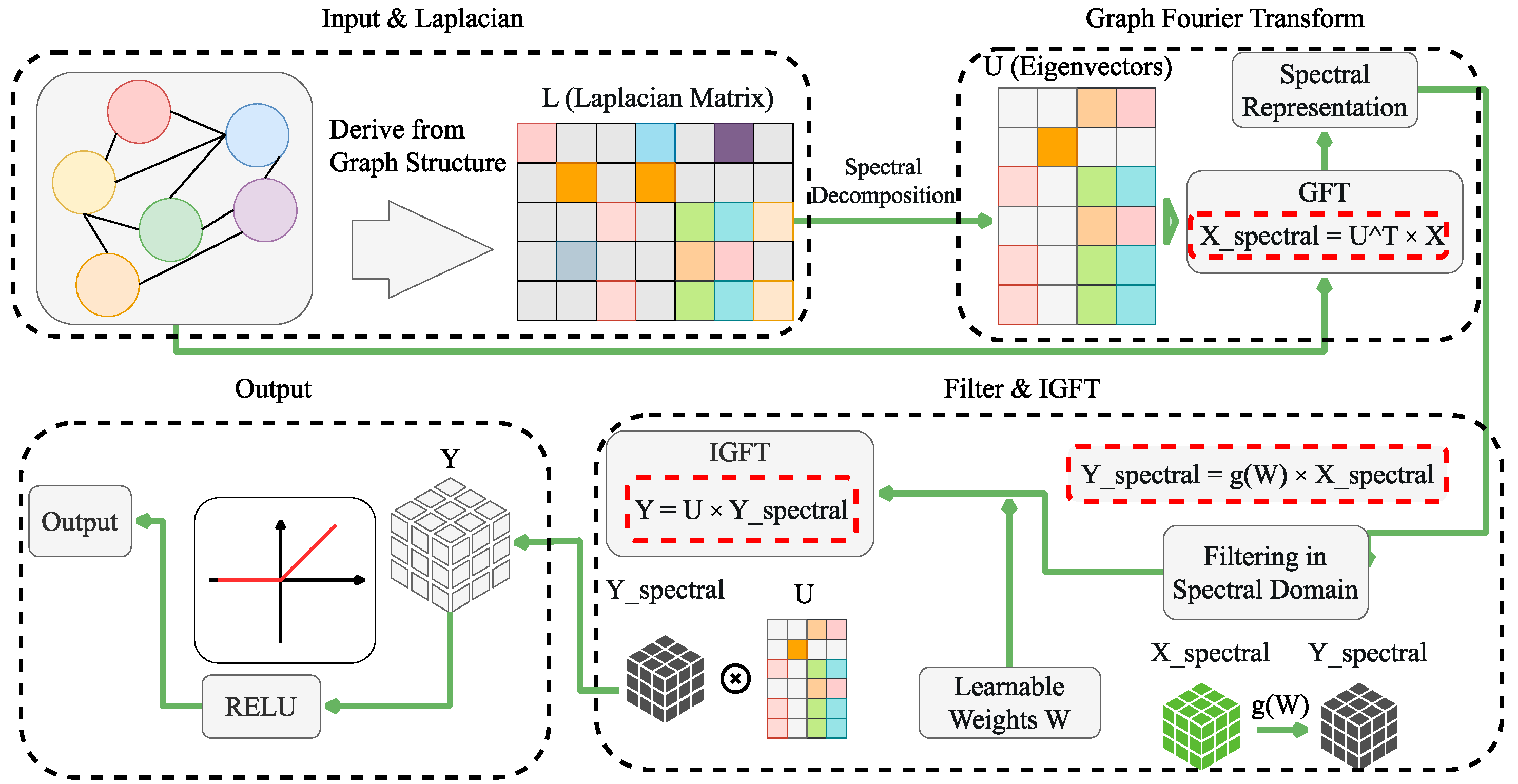
Our model employs Spectral Graph Convolution (SGC) as the core mechanism for spatial reasoning, leveraging graph signal processing theory to transform spatial dependencies into the spectral domain. By decomposing graph signals through eigendecomposition of the graph Laplacian, SGC efficiently captures complex inter-turbine relationships that are difficult to model in the vertex domain. As shown in Figure 1, this spectral approach naturally accommodates the non-Euclidean spatial structure of wind farm networks while maintaining computational efficiency.

As shown in Figure 4, The operation is founded on the spectral decomposition of the graph Laplacian, $L=D-A$, where $A$ is the adjacency matrix and $D$ is the diagonal degree matrix. The eigendecomposition of the Laplacian yields $L=U\Lambda U^T$, where the matrix of eigenvectors $U$ forms an orthonormal basis known as the Graph Fourier Basis. This basis is fundamental, allowing us to define Fourier transforms for signals residing on the graph. Given a graph signal $X\in {ℝ}^{N\times C_{in}}$, we first project it onto the spectral basis via the Graph Fourier Transform (GFT) to obtain its spectral representation, $X_{spectral}$:

$$X_{spectral}=U^{T}X$$

(6)

In this spectral domain, the convolution operation simplifies to a filtering process. We implement this filter as a learnable weight matrix $W\in {ℝ}^{C_{in}\times C_{out}}$, which modulates the spectral components of the signal. The filtered signal, $Y_{spectral}$, is then computed through a linear transformation:

$$Y_{spectral}=X_{spectral}W$$

(7)

Finally, the resulting signal is transformed back to the vertex domain using the Inverse Graph Fourier Transform (IGFT), which is achieved by multiplying with the basis matrix $U$:

$$Y=U{Y}_{spectral}$$

(8)

The entire spectral graph convolution, encompassing the transform, filtering, and inverse transform, is encapsulated into a single operation, followed by a ReLU activation function to introduce non-linearity. This complete formulation enables the model to learn complex spatial patterns by adaptively filtering the graph signal across its frequency components.

2.6. Output Layer for Multi-Step Prediction

Following the deep feature extraction performed by the stacked spatio-temporal blocks, a dedicated output layer is employed to transform the learned high-dimensional representations into the final multi-step power forecast. This final module is responsible for aggregating the processed features and mapping them to the desired prediction horizon.

The process begins by synthesizing the rich spatio-temporal features. Given the output tensor from the final spatio-temporal block, which contains feature representations for all turbine and weather nodes, we first perform a spatial aggregation step. Specifically, the features corresponding only to the turbine nodes are isolated and then averaged across the node dimension. This yields a unified temporal feature map that encapsulates the collective state and dynamics of the entire wind farm.

This aggregated feature map is subsequently flattened into a single vector to serve as input for a Multi-Layer Perceptron (MLP). The MLP, acting as the prediction head, consists of two fully connected layers. The first layer projects the high-dimensional feature vector into a dense hidden representation, followed by a ReLU activation and a dropout layer to enhance generalization and mitigate overfitting. The second linear layer then maps this intermediate representation to the final output vector $\hat{Y}\in {ℝ}^{T_{pred}}$, where $T_{pred}$ is the length of the prediction horizon. Each element in $\hat{Y}$ corresponds to the predicted total power of the wind farm for a specific future time step. The complete operation can be formulated as:

$$\hat{Y}=MLP(Flatten(Mea{n}_{nodes}(X_{turb})))$$

(9)

where $X_{turb}$ is the feature tensor for the turbine nodes and $Mea{n}_{nodes}$ is the averaging operation across the turbine node dimension.

3. Dataset Description

This section describes the self-collected dataset used for model validation and outlines the comprehensive preprocessing pipeline designed to handle real-world wind energy data complexities.

3.1. DMSWPF Dataset

This study utilizes a comprehensive, self-collected dataset, hereafter referred to as the DMSWPF (Dynamic-Meteorological-Static Wind Power Forecasting) dataset. It comprises two primary components: high-resolution SCADA data from a wind farm in Central China and corresponding meteorological forecast data from ECMWF.

The wind turbine data includes SCADA records from 29 wind turbines, with dynamic variables sampled at 15-min intervals, including turbine-specific cut-in wind speed and active power generation. Static variables consist of the precise geographic coordinates (latitude and longitude) and elevation for each turbine, which are crucial for modeling spatial relationships. The data spans from January 2023 to September 2024, totaling 58,273 timesteps.

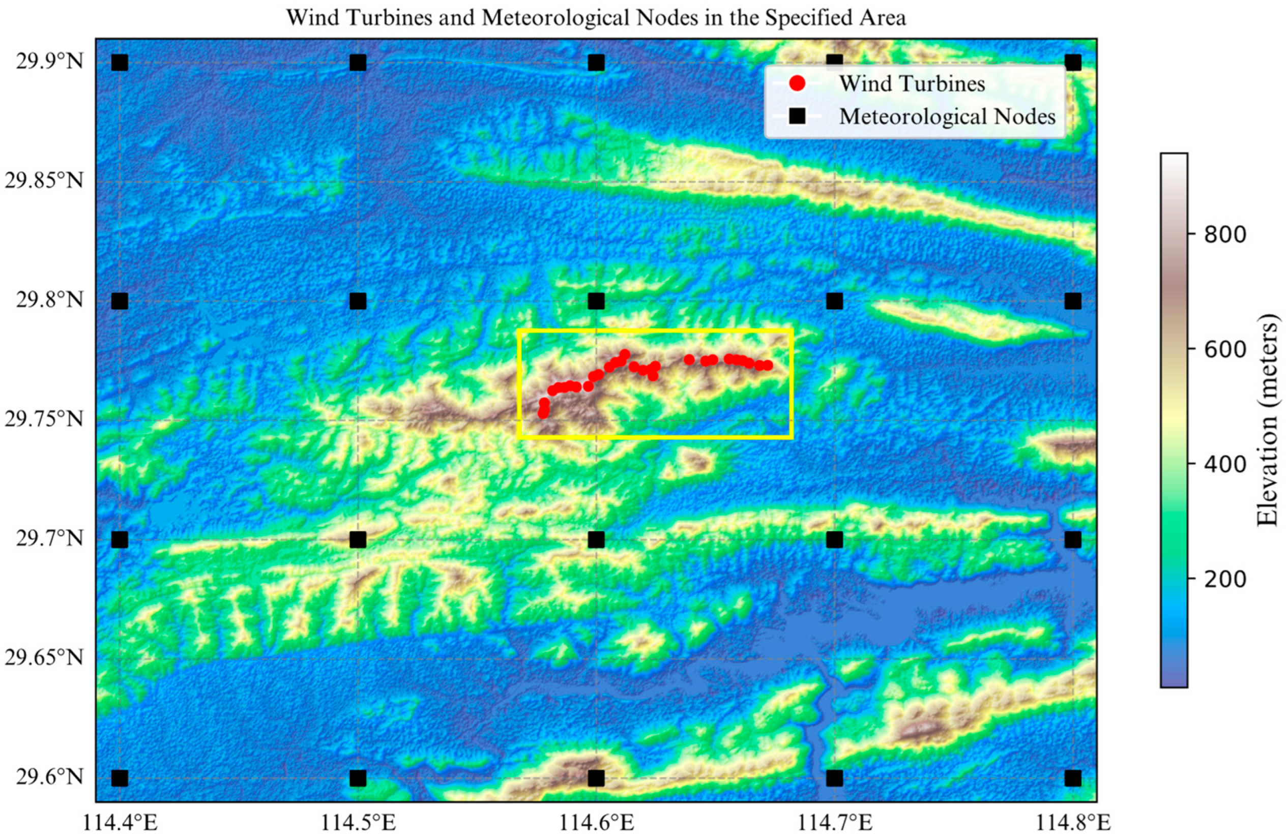
To provide rich contextual information, we incorporated gridded numerical weather prediction (NWP) data sourced from the European Centre for Medium-Range Weather Forecasts (ECMWF). This data covers a 4 × 5 grid of 20 meteorological nodes, strategically overlaying the wind farm region with a high spatial resolution of 0.1° × 0.1°. Each node provides 21 distinct meteorological features, including multi-level wind components (e.g., at 10 m, 100 m, 200 m), temperature, solar radiation, and atmospheric pressure. The temporal coverage and resolution are perfectly aligned with the turbine data, ensuring a one-to-one correspondence for each time step. The inclusion of diverse meteorological variables beyond just wind speed is intended to empower the model to discover and leverage complex, non-linear. relationships that influence power generation.

3.2. Data Processing

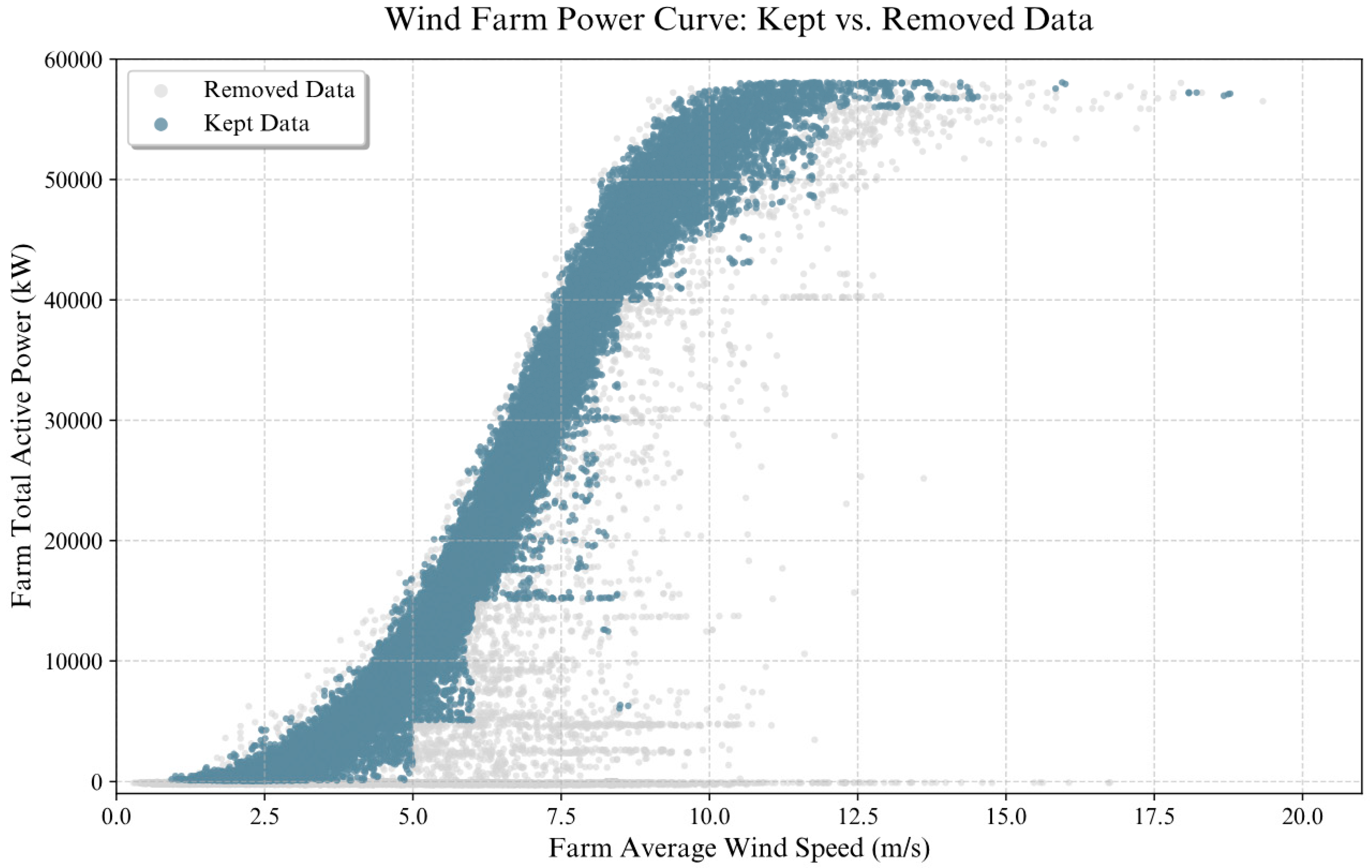
SCADA power streams are, by nature, messy. Figure 5 makes this plain: power versus wind speed appears as a diffuse scatter rather than a tidy curve. Flat-topped plateaus signal grid curtailment; the broad underperformance cloud reflects instrumentation issues, yaw misalignment, off-optimal tip-speed ratios, or wake losses; a dense knot at zero power marks planned or fault-induced standstills. Our preprocessing is disciplined yet pragmatic. SCADA power streams are messy, and Figure 5 visualizes the remedy rather than the raw problem: a hybrid cleaning that separates kept points (blue) from removed points (gray) on the farm power curve. We excise shutdown clusters near zero, a diffuse low-power band at moderate wind speeds, and interior islands of inconsistent performance—including the knot around 6–8 m/s and 5–11 MW—while preserving the outer envelope of the curve. Flat-topped curtailment interiors are pruned, but points that define the upper hull are retained. Operationally, we combine simple rule screens, a 2-D density filter, and an explicit envelope safeguard (high-quantile power within wind-speed bins) to avoid eroding the rated-power shoulder. The resulting keep set is cleaner and more monotone, facilitating power-curve modeling and downstream analysis.

Figure 6 provides a topographical map of the study area, illustrating the core challenge of spatial heterogeneity. The wind turbines (red dots) are shown densely deployed along the high-elevation mountain ridges, while the meteorological nodes (black squares) are sparsely distributed across the entire area in a coarse grid. This spatial heterogeneity poses a challenge for precise wind power forecasting, as it is difficult to accurately map the sparse meteorological data to the location of each individual turbine. To address this issue, we need to construct a Unified Heterogeneous Graph Structure. This graph structure treats each wind turbine and meteorological node as a node in the graph, with edges defined by the geospatial relationships between them, thereby capturing their spatial correlations within a single, unified view. In this way, a model can learn how meteorological information propagates from the sparse meteorological nodes to influence the dense cluster of wind turbines, capturing more refined and localized weather features for each turbine and ultimately improving forecasting accuracy.

Zero-variance features are removed, as they add no signal and can skew normalization. All remaining numeric covariates—turbine and meteorological—are standardized with a z-score transform (StandardScaler: zero mean, unit variance) to stabilize optimization and prevent magnitude-driven dominance. Robust or per-turbine scaling can be defensible under heavy tails or strong site heterogeneity, but in this setting global z-scores were sufficient. Temporal dependencies are preserved through a sliding-window design. Each sample uses 24 steps (6 h) of history to predict the next 16 steps (4 h)—long enough to capture ramps and diurnal cues, short enough to keep local stationarity plausible. Quality control is strict: any window containing NaN or ±∞ in either inputs or target is discarded in full. This sacrifices some coverage yet yields clean supervision without loss masking. Finally, sequences are split chronologically into training/validation/test at 80/10/10. Respecting time’s arrow avoids future leakage and mirrors operational deployment; rolling-origin evaluation could offer broader stress testing, but a single ordered holdout provides a clear, reproducible benchmark.

4. Experiment and Performance Evaluation

We evaluate the proposed SA-STGCN on our self-collected wind farm dataset through comprehensive experiments against six representative deep learning baselines: wavelet_STGCN, (Graph Attention Network) GAT, (Spatio-Temporal Transformer) ST_TRANSFORMER, BASIC_TRANSFORMER, (Attention LSTM) ATTN-LSTM, and SIMPLE_LSTM, (Light Gradient Boosting Machine) LGBM. These models represent state-of-the-art approaches in spatio-temporal forecasting and provide strong comparative benchmarks. All models undergo identical data preprocessing and hyperparameter optimization to ensure fair evaluation. Performance is assessed using Mean Absolute Error (MAE) and Root Mean Square Error (RMSE) metrics. The experimental results demonstrate that SA-STGCN consistently outperforms these baselines, showcasing superior accuracy and robustness in capturing complex wind power dynamics.

4.1. Settings

The experiments were conducted on a high-performance computing platform featuring an NVIDIA RTX 4090 (24GB VRAM) with CUDA 12.4 support, implemented within the PyTorch 2.8.0 framework. The forecasting task was defined as predicting the total wind farm power output for a 16-step future horizon (equivalent to 4 h, assuming 15-min intervals) based on a 24-step historical input window (6 h). The entire dataset was partitioned into training and validation sets with an 80/20 split.

All models were implemented in PyTorch and trained on a CUDA-enabled GPU. Optimization was performed using the AdamW optimizer, configured with a learning rate of 1 × 10⁻⁴ and a weight decay of 1 × 10⁻⁵, minimizing a Mean Squared Error (MSE) loss function. To accelerate training and improve numerical stability, automatic mixed precision (AMP) with gradient scaling was employed. The training was conducted with a batch size of 128 for a maximum of 50 epochs. An early stopping mechanism with a patience of 10 epochs was instituted to prevent overfitting, monitored on the validation loss. This was complemented by a ReduceLROnPlateau learning rate scheduler, which reduced the learning rate by a factor of 0.5 after 3 consecutive epochs with no improvement in validation RMSE.

The architecture of our proposed Spectral Attentive STGCN (SA-STGCN) model is configured as follows. It is built with a hidden dimension of 64 and consists of 3 stacked STGCN blocks. For the feature augmentation stage, we employ a Daubechies 4 (‘db4’) wavelet transform with a single decomposition level. Within each STGCN block, the temporal attention mechanism is implemented with 4 attention heads and operates globally across the entire 24-step input sequence to capture long-range dependencies. A dropout rate of 0.1 is applied within the attention module. Finally, the output projection network utilizes an intermediate layer of 512 dimensions followed by a dropout layer with a rate of 0.2 before generating the final 16-step forecast. The performance of each model was quantified using four metrics: Mean Absolute Error (MAE) and Root Mean Squared Error (RMSE), both reported in Megawatts (MW), R² Score, and a Day-Ahead Accuracy Rate, calculated relative to the farm’s rated capacity of 58 MW.

4.2. Evaluation Metrics

In this research, we employ multiple evaluation metrics to comprehensively assess the performance of prediction models. These metrics are categorized into two groups: Error Metrics and Predictive Accuracy Metrics. Error Metrics include the following:

The mean absolute error (MAE) measures the average absolute difference between actual values y_i and predicted values ${\hat{y}}_i$, providing an intuitive sense of overall prediction error:

$$MAE={\displaystyle \frac{1}{n}}{\displaystyle \sum _{i=1}^n\left|y_i-{\hat{y}}_i\right|}$$

(10)

The root mean squared error (RMSE) is similar but emphasizes larger errors due to the squaring operation:

$$RMSE=\sqrt{{\displaystyle \frac{1}{n}}{\displaystyle \sum _{i=1}^n{(y_i-{\hat{y}}_i)}^2}}$$

(11)

The coefficient of determination (R²) quantifies how well the model explains the variance in the target variable:

$$R^2=1-{\displaystyle \frac{{\displaystyle \sum _{i=1}^n{(y_i-{\hat{y}}_i)}^2}}{{\displaystyle \sum _{i=1}^n{(y_i-\overline{y})}^2}}}$$

(12)

here, sgn(⋅) is the sign function, returning +1 if the argument is positive, −1 if negative, and 0 if zero, indicating whether two pairs are concordant or discordant. Finally, Mutual Information (MI), denoted as ($I(Y;\hat{Y})$) quantifies the amount of information shared between actual and predicted sequences:

$$I(Y;\hat{Y})={\displaystyle \sum _{y\in Y}{\displaystyle \sum _{\hat{y}\in \hat{Y}}p}}(y,\hat{y})\log \left({\displaystyle \frac{p(y,\hat{y})}{p(y)p(\hat{y})}}\right)$$

(13)

In this expression, $p(y,\hat{y})$: Joint probability distribution of actual and predicted values; $p(y)$, $p(\hat{y})$: Marginal probability distributions. This metric captures both linear and non-linear dependencies, making it particularly useful for assessing complex model behaviors. By applying these error and predictive accuracy metrics, we are able to comprehensively evaluate the performance of the proposed prediction models.

4.3. Experimental Results

We evaluate 4-hour-ahead wind power forecasting (16 future steps) using 24 historical steps as input on a self-curated SCADA dataset. All models share the same splits, training pipeline, and a conservative preprocessing protocol that flags curtailment/inefficiency/shutdowns and applies short-window forward/back filling to preserve autocorrelation without fabricating high-frequency content. We benchmark the proposed SA-STGCN against (Graph Attention Network) GAT, (Spatio-Temporal Transformer) ST_TRANSFORMER, BASIC_TRANSFORMER, (Attention LSTM) ATTN-LSTM, and SIMPLE_LSTM, (Light Gradient Boosting Machine) LGBM.

Table 1. Performance comparison of time series forecasting models.

Model	MAE	RMSE	R2	MI
SA-STGCN	1.52 ± 0.08	2.31 ± 0.15	0.94 ± 0.012	1.61 ± 0.13
WAVELET_STGCN	1.74 ± 0.1	2.71 ± 0.2	0.93 ± 0.02	1.53 ± 0.13
GAT	1.95 ± 0.1	3.10 ± 0.13	0.90 ± 0.05	1.45 ± 0.1
LGBM	2.12 ± 0.1	3.35 ± 0.15	0.88 ± 0.07	1.41 ± 0.11
ST_TRANSFORMER	2.30 ± 0.1	3.66 ± 0.15	0.86 ± 0.08	1.37±
BASIC_TRANSFORMER	2.76 ± 0.1	4.41 ± 0.19	0.80 ± 0.05	1.28 ± 0.08
ATTN-LSTM	3.19 ± 0.12	5.14 ± 0.21	0.75 ± 0.05	1.17 ± 0.04
SIMPLE_LSTM	3.59 ± 0.11	5.67 ± 0.2	0.71 ± 0.04	1.09 ± 0.06

reports the quantitative results and Figure 7 visualizes them.

4.4. Evaluation Results and Analysis

As illustrated in Figure 7 and Table 1, the comparison across seven competing models reveals a striking advantage of the proposed SA-STGCN framework. Among all contenders, it consistently delivered the most accurate predictions, securing the lowest error rates (MAE 1.52, RMSE 2.31) while achieving the highest accuracy and information efficiency (R² 0.94, MI 1.61). Against the next-best WAVELET_STGCN, these differences translate into 12.6% and 14.8% reductions in MAE and RMSE, respectively, accompanied by a more subtle—yet still meaningful—rise in R² from 0.93 to 0.94. Such improvements, though numerically modest in R², are backed by double-digit drops in absolute error, pointing to real, not cosmetic, advances. The implication is straightforward: coupling spatial attention with spatio-temporal graph convolution allows the model to grasp both structural dependency and temporal dynamics in a synergistic way.

This advantage is magnified when SA-STGCN is set against architectures that do not explicitly embed graph structure. Purely sequential models, whether Transformer-based or recurrent, fall noticeably behind. Against ST_TRANSFORMER, SA-STGCN reduces MAE and RMSE by roughly one--third, and against BASIC_TRANSFORMER the gap widens to nearly half, with R² surging from 0.80 to 0.94. The contrast grows even sharper for recurrent variants: compared with SIMPLE_LSTM, error rates collapse by nearly 60%, while predictive power (R²) leaps from 0.71 to 0.94. Even models enhanced with graph attention (GAT) or attention-augmented LSTMs confirm this same pattern—the absence of a unified spatio-temporal perspective proves costly. Interestingly, the tree-based LGBM slots into an intermediate position. It performs noticeably better than traditional sequence learners, with R² 0.88 and MI 1.41, yet it lags behind specialized graph architectures. This is hardly surprising: gradient boosting captures nonlinear effects with finesse, but it lacks the structural machinery to encode long-range temporal correlations or spatial interdependencies that graph neural networks exploit almost effortlessly.

Taken together, the performance hierarchy is unambiguous. Methods that integrate spatial dependence with temporal evolution—exemplified by SA-STGCN and WAVELET_STGCN—consistently take the lead. Some might regard a 0.01 improvement in R², from 0.93 to 0.94, as trivial in a saturating regime; however, this view overlooks the paired double-digit reductions in MAE and RMSE. In practice, such improvements represent tangible gains in reliability and robustness, the kind that can shift decision-making outcomes in real datasets. This blend of subtle statistical refinement with substantial application-level benefit is precisely what signals a genuine advancement rather than an exercise in numerical cosmetics.

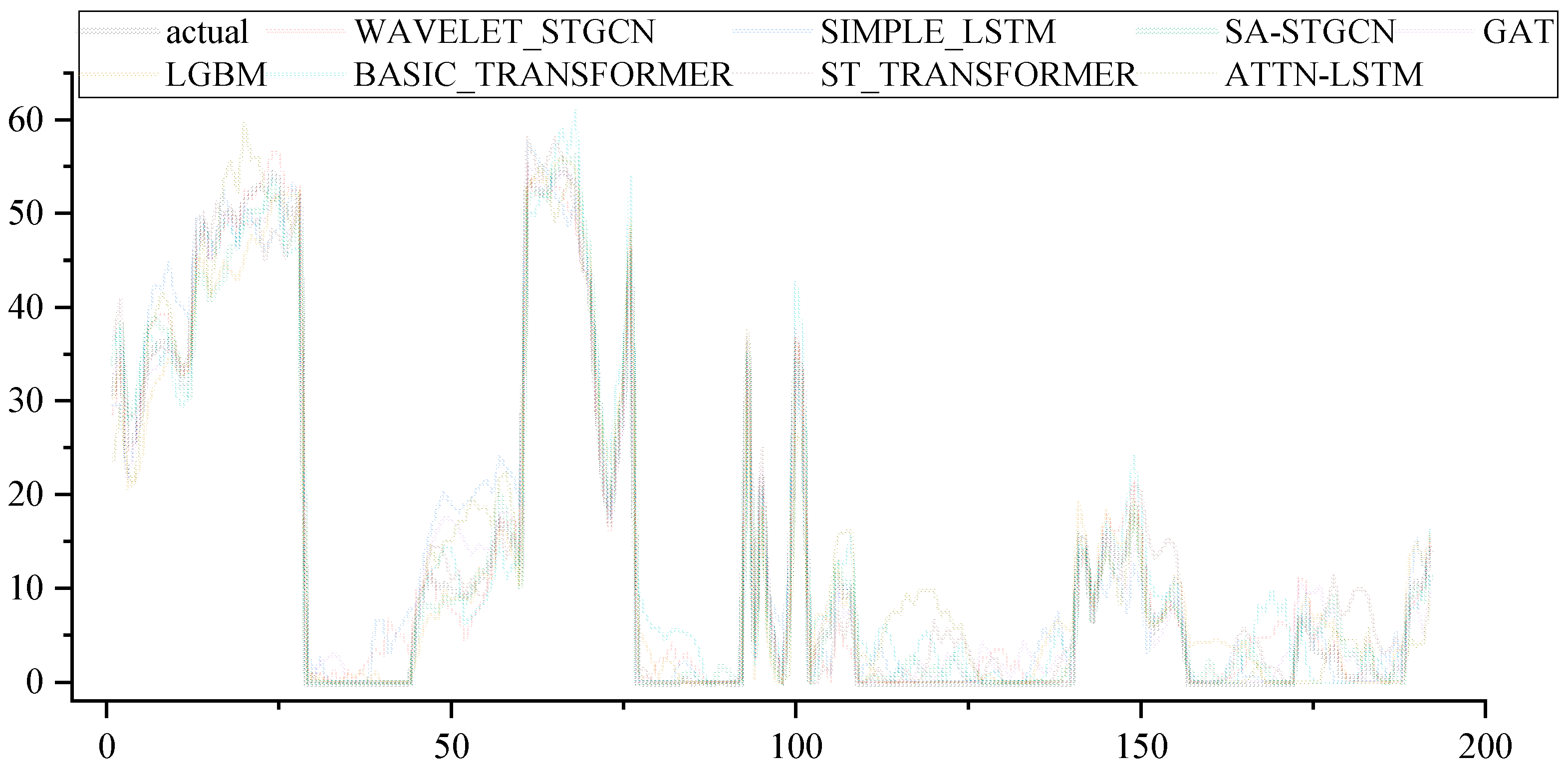
Figure 8 comparison of predicted wind power outputs from different models against the ground truth (black curve) over a representative period characterized by sharp fluctuations. The results clearly demonstrate that the proposed SA-STGCN model (green curve) achieves the closest alignment with the actual values, successfully capturing the rapid variations and peak magnitudes in power output. In contrast, other benchmark models exhibit noticeable deviations, with some predictions showing evident lags during steep ramps, while others tend to underestimate peak values or display unstable tracking in highly volatile intervals. This indicates the superior ability of SA-STGCN to model spatiotemporal dependencies and maintain robustness under highly dynamic conditions.

The computational cost analysis in

Table 2. Training and inference cost analysis of various models.

Model	Training Time (s)	Inference Time (s)	Peak GPU Memory (MB)
ST_TRANSFORMER	1210.5	8.2	16,550.2
SA-STGCN	1105.3	7.4	15,210.6
WAVELET_STGCN	985.1	6.9	8150.0
GAT	870.4	6.3	7100.5
BASIC_TRANSFORMER	915.0	6.5	7330.0
ATTN-LSTM	750.2	5.8	5540.8
SIMPLE_LSTM	550.6	4.8	4120.4
LGBM	75.3	1.5	900

reveals a clear stratification of models according to resource demands. At the upper tier, ST_TRANSFORMER and SA-STGCN are the most resource-intensive, requiring over 1100 s of training and more than 15 GB of GPU memory, a direct consequence of their heavy attention mechanisms. At the opposite end, LSTM-based models such as SIMPLE_LSTM demonstrate far greater efficiency, with training times under 600 s and modest memory footprints around 4 GB. Intermediate architectures—WAVELET_STGCN, GAT, BASIC_TRANSFORMER, and ATTN-LSTM—strike a balance, incurring moderate costs of 700–1000 s and 5–8 GB memory. Notably, the inclusion of LGBM sharpens this contrast: with just 75 s of training, a 1.5-s inference, and peak memory under 1 GB, it represents the extreme low-cost frontier. While this efficiency highlights its practicality in constrained environments, its lightweight profile also explains why it cannot rival graph-based deep models in capturing rich spatio-temporal dependencies.

4.5. Ablation Experiments

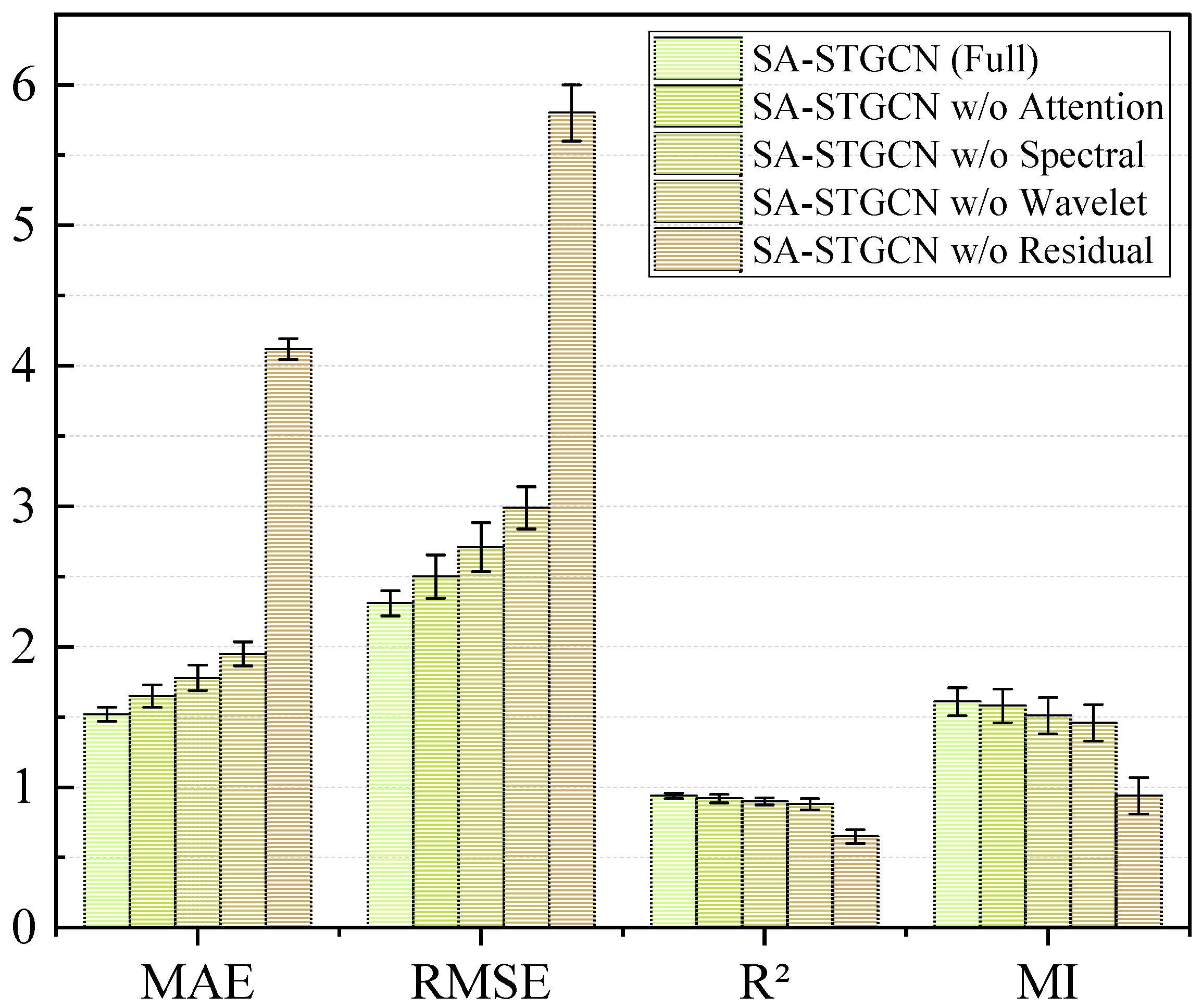
To rigorously validate the effectiveness and necessity of each key component within our proposed SA-STGCN model, we have conducted a comprehensive ablation study, with the results presented in

Table 3. Ablation experiments comparison on error metrics and predictive accuracy.

Model	MAE	RMSE	R2	MI
SA-STGCN (Full)	1.52 ± 0.05	2.31 ± 0.09	0.94 ± 0.02	1.61 ± 0.1
SA-STGCN w/o Attention	1.65 ± 0.08	2.50 ± 0.16	0.92 ± 0.03	1.58 ± 0.12
SA-STGCN w/o Spectral	1.78 ± 0.09	2.72 ± 0.18	0.90 ± 0.03	1.51 ± 0.13
SA-STGCN w/o Wavelet	1.95 ± 0.085	2.99 ± 0.15	0.88 ± 0.04	1.46 ± 0.13
SA-STGCN w/o Residual	4.12 ± 0.075	5.80 ± 0.2	0.65 ± 0.05	0.94 ± 0.12

and Figure 9 This study was designed to systematically deconstruct the model and quantify the contribution of each module to the overall predictive performance. To ensure a fair and controlled comparison, all model variants were trained and evaluated under identical experimental conditions, including the same dataset, data preprocessing, and hyperparameter settings. Our complete proposed model, SA-STGCN (Full), serves as the benchmark representing the optimal performance achieved when all components work in synergy. Against this benchmark, we evaluated several ablated versions. The ‘SA-STGCN w/o Attention’ variant was developed by removing the self-attention mechanism to measure its impact on identifying salient spatiotemporal features. Similarly, the ‘SA-STGCN w/o Spectral’ model excluded the spectral graph convolution layers to evaluate the contribution of graph-based spatial analysis. To test the role of multi-resolution temporal analysis, we implemented the ‘SA-STGCN w/o Wavelet’ variant, which omits the wavelet transform component. Finally, to demonstrate the critical role of residual learning in enabling a deep architecture and facilitating gradient flow, we tested a ‘SA-STGCN w/o Residual’ model with all residual connections removed. By comparing the performance metrics of these ablated configurations against the full model, any significant performance degradation directly quantifies the positive and necessary contribution of the removed component to the model’s overall success.

Beyond just improving predictive accuracy, the components of SA-STGCN also significantly enhance the model’s interpretability. The temporal attention mechanism, for instance, highlights which past time steps have the greatest influence on the forecast, offering a transparent view of the key historical conditions that drive sudden ramps or sustained fluctuations in wind power. Simultaneously, the spectral graph convolution sheds light on the spatial dimension by capturing non-local correlations among distant wind turbines that are jointly affected by large-scale meteorological systems. Together, these components provide valuable insights into the temporal and spatial patterns underlying the model’s predictions.

The conclusion from our ablation study is that all components of the SA-STGCN model—the attention mechanism, spectral graph convolution, wavelet transform, and residual connections—are effective and necessary, working in synergy to achieve optimal performance. The variant without residual connections (‘SA-STGCN w/o Residual’) exhibited the most substantial performance degradation, underscoring that these connections are the most critical component of the architecture. This is because residual connections are fundamental for training deep models by providing identity shortcut paths that ensure stable gradient propagation during backpropagation, effectively mitigating the vanishing gradient problem. Without them, our 3-block deep model becomes significantly harder to optimize, leading to poor convergence and a collapse in predictive accuracy. While less severe, the performance drops in other variants still confirm the value of the wavelet transform for multi-resolution analysis, spectral graph convolution for capturing complex spatial correlations, and the attention mechanism for focusing on salient temporal features. This comprehensive analysis validates the rationality and integrity of our model’s design.

5. Conclusions

This paper presents a novel deep learning architecture, the Spectral Attentive Spatio-Temporal Graph Convolutional Network (SA-STGCN), designed for high-precision wind power forecasting. The model integrates Wavelet Transform, Temporal Attention, and Spectral Graph Convolutions within a unified framework to effectively capture complex spatiotemporal dependencies in wind power systems.

Experimental validation demonstrates the model’s superior performance, achieving a Mean Absolute Error (MAE) of 1.52 and Root Mean Squared Error (RMSE) of 2.31. These results validate the model’s capacity for reliable and precise forecasting in real-world wind power prediction scenarios.

The effectiveness of SA-STGCN stems from its multi-component architecture. The wavelet transform decomposes input signals into frequency sub-bands, enabling simultaneous capture of long-term trends and short-term fluctuations. The Temporal Attention mechanism adaptively weights historical time steps, focusing computational resources on the most predictive temporal patterns. The Spectral Graph Convolution operates in the graph Fourier domain to model global spatial correlations across the turbine network, transcending the locality constraints of traditional message-passing approaches.

Future research directions include developing dynamic graph structures that incorporate time-varying physical factors such as wind direction patterns, enhancing computational efficiency through architectural optimization, and extending the framework to long-term and probabilistic forecasting scenarios. Additionally, its application should be tested on other renewable sources like solar power, where precise forecasting is equally critical for resource management [32]. These advances will further improve forecasting accuracy and support more effective grid management strategies for renewable energy integration.

References

1. Zhao, B.; Zhang, Y.; Li, Z.; Han, X.; Liu, H.; Dong, C.; Wang, J.; Liu, C.; Xia, Y. Spatial correlation learning based on graph neural network for medium-term wind power forecasting. Energy 2024, 296, 131164. [Google Scholar] [CrossRef]
2. Global Wind Energy Council. Global Wind Report 2025; GWEC: Brussels, Belgium, 2024. [Google Scholar]
3. Kim, J.; Shin, H.-J.; Lee, K.; Hong, J. Enhancement of ANN-based wind power forecasting by modification of surface roughness parameterization over complex terrain. J. Environ. Manag. 2024, 362, 121246. [Google Scholar] [CrossRef]
4. Mei, H.; Zhu, Q.; Cao, W. A TSFLinear model for wind power prediction with feature decomposition-clustering. Renew. Energy 2025, 248, 123142. [Google Scholar] [CrossRef]
5. Wang, R.; Wu, J.; Cheng, X.; Liu, X.; Qiu, H. Enhancing spatiotemporal wind power forecasting with meta-learning in data-scarce environments. Eng. Appl. Artif. Intell. 2025, 156, 111121. [Google Scholar] [CrossRef]
6. Chen, N.; Qian, Z.; Nabney, I.T.; Meng, X. Wind power forecasts using Gaussian processes and numerical weather prediction. IEEE Trans. Power Syst. 2014, 29, 656–665. [Google Scholar] [CrossRef]
7. Jiang, Y.; Chen, X.; Yu, K.; Liao, Y. Short-term wind power forecasting using hybrid method based on enhanced boosting algorithm. J. Mod. Power Syst. Clean Energy 2017, 5, 126–133. [Google Scholar] [CrossRef]
8. Chen, P.; Pedersen, T.; Bak-Jensen, B.; Chen, Z. ARIMA-based time series model of stochastic wind power generation. IEEE Trans. Power Syst. 2010, 25, 667–676. [Google Scholar] [CrossRef]
9. Singh, A.R.; Kumar, R.S.; Bajaj, M.; Khadse, C.B.; Zaitsev, I. Machine learning-based energy management and power forecasting in grid-connected microgrids with multiple distributed energy sources. Sci. Rep. 2024, 14, 19207. [Google Scholar] [CrossRef]
10. Morgoeva, A.D.; Morgoev, I.D.; Klyuev, R.V.; Kochkovskaya, S.S. Forecasting Hourly Electricity Generation of Solar Power Plants Using Machine Learning Algorithms. Bull. Tomsk. Polytech. Univ. Geo-Resour. Eng. 2023, 334, 7–19. [Google Scholar] [CrossRef]
11. Dong, M.; Sun, M.; Song, D.; Huang, L.; Yang, J.; Joo, Y.H. Real-time detection of wind power abnormal data based on semi-supervised learning Robust Random Cut Forest. Energy 2022, 257, 124761. [Google Scholar] [CrossRef]
12. Dong, L.; Wang, L.; Khahro, S.F.; Gao, S.; Liao, X. Wind power day-ahead prediction with cluster analysis of NWP. Renew. Sustain. Energy Rev. 2016, 60, 1206–1212. [Google Scholar] [CrossRef]
13. Kolkmann, S.; Ostmeier, L.; Weber, C. Modeling multivariate intraday forecast update processes for wind power. Energy Econ. 2024, 139, 107890. [Google Scholar] [CrossRef]
14. Peng, X.; Li, Y.; Tsung, F. A graph attention network with spatio-temporal wind propagation graph for wind power ramp events prediction. Renew. Energy 2024, 236, 121280. [Google Scholar] [CrossRef]
15. Zhao, Y.; Liao, H.; Pan, S.; Zhao, Y. Interpretable multi-graph convolution network integrating spatio-temporal attention and dynamic combination for wind power forecasting. Expert Syst. Appl. 2024, 255, 124766. [Google Scholar] [CrossRef]
16. Yu, C.; Yan, G.; Yu, C.; Zhang, Y.; Mi, X. A multi-factor driven spatiotemporal wind power prediction model based on ensemble deep graph attention reinforcement learning networks. Energy 2023, 263, 126034. [Google Scholar] [CrossRef]
17. Zhang, J.; Li, H.; Cheng, P.; Yan, J. Interpretable Wind Power Short-Term Power Prediction Model Using Deep Graph Attention Network. Energies 2024, 17, 384. [Google Scholar] [CrossRef]
18. Xie, Y.; Zheng, J.; Taylor, G.; Hulak, D. A short-term wind power prediction method via self-adaptive adjacency matrix and spatiotemporal graph neural networks. Comput. Electr. Eng. 2024, 120, 109715. [Google Scholar] [CrossRef]
19. Hou, G.; Li, Q.; Huang, C. Spatiotemporal forecasting using multi-graph neural network assisted dual domain transformer for wind power. Energy Convers. Manag. 2025, 325, 119393. [Google Scholar] [CrossRef]
20. Liang, X.; Hu, Z.; Zhang, J.; Chen, H.; Gu, Q.; You, X. Developing a robust wind power forecasting method: Integrating data repair, feature screening, and economic impact analysis for practical applications. Renew. Energy 2025, 247, 122775. [Google Scholar] [CrossRef]
21. Dong, F.; Ju, S.; Liu, J.; Yu, D.; Li, H. An ultra-short-term wind power robust prediction method considering the periodic impact of wind direction. Renew. Energy 2025, 247, 122983. [Google Scholar] [CrossRef]
22. He, Y.; Yu, N.; Wang, B. Online probability density prediction of wind power considering virtual and real concept drift detection. Appl. Energy 2025, 396, 126318. [Google Scholar] [CrossRef]
23. Li, C.; Guo, Y.; Xu, Y. A double deep reinforcement learning-based adaptive framework for decision-optimal wind power interval prediction. Energy 2025, 329, 136661. [Google Scholar] [CrossRef]
24. Wu, S.; Chen, Y.; He, X.; Wang, Z.; Liu, X.; Fu, Y. Cabin: A collaborative and adaptive framework for wind power forecasting integrating ambient variables. Energy 2025, 335, 137753. [Google Scholar] [CrossRef]
25. Qiao, B.; Liu, J.; Wu, P.; Teng, Y. Wind power forecasting based on variational mode decomposition and high-order fuzzy cognitive maps. Appl. Soft Comput. 2022, 129, 109586. [Google Scholar] [CrossRef]
26. Gao, J.; Xing, H.; Wang, Y.; Liu, G.; Cheng, B.; Zhang, D. Ultra-short-term wind power prediction based on hybrid denoising with improved CEEMD decomposition. Renew. Energy 2025, 251, 123352. [Google Scholar] [CrossRef]
27. Qu, Z.; Li, J.; Hou, X.; Gui, J. A D-stacking dual-fusion, spatio-temporal graph deep neural network based on a multi-integrated overlay for short-term wind-farm cluster power multi-step prediction. Energy 2023, 281, 128289. [Google Scholar] [CrossRef]
28. Qiu, H.; Shi, K.; Wang, R.; Zhang, L.; Liu, X.; Cheng, X. A novel temporal–spatial graph neural network for wind power forecasting considering blockage effects. Renew. Energy 2024, 227, 120499. [Google Scholar] [CrossRef]
29. Wang, J.; Kou, M.; Li, R.; Qian, Y.; Li, Z. Ultra-short-term wind power forecasting jointly driven by anomaly detection, clustering and graph convolutional recurrent neural networks. Adv. Eng. Inform. 2025, 65, 103137. [Google Scholar] [CrossRef]
30. Liao, W.; Wang, S.; Bak-Jensen, B.; Pillai, J.R.; Yang, Z.; Liu, K. Ultra-short-term interval prediction of wind power based on graph neural network and improved bootstrap technique. J. Mod. Power Syst. Clean Energy 2023, 11, 1100–1114. [Google Scholar] [CrossRef]
31. Qu, K.; Si, G.; Wang, Q.; Xu, M.; Shan, Z. Improving economic operation of a microgrid through expert behaviors and prediction intervals. Appl. Energy 2025, 383, 125391. [Google Scholar] [CrossRef]
32. Jovanovic, L.; Bacanin, N.; Petrovic, A.; Zivkovic, M.; Antonijevic, M.; Gajic, V.; Elsayed, M.M.; Abouhawwash, M. Exploring artificial intelligence potential in solar energy production forecasting: Methodology based on modified PSO optimized attention augmented recurrent networks. Sustain. Comput. Inform. Syst. 2025, 47, 101174. [Google Scholar] [CrossRef]
Figure 3. Illustration of the self-attention mechanism.
Energies 18 05315 g003
Figure 4. The architecture of the spectral graph convolution layer.
Energies 18 05315 g004
Figure 5. Wind farm power curve after hybrid cleaning. Blue points are retained; gray points are removed by rule-based screens and a density filter. Curtailment interiors and underperforming islands are culled, while the envelope of the curve is preserved.
Energies 18 05315 g005
Figure 6. Topographical map and spatial distribution of wind turbines and meteorological nodes in the study area.
Energies 18 05315 g006
Figure 7. Experimental results comparison of overall forecasting errors of each model.
Energies 18 05315 g007
Figure 8. Evaluating model accuracy in predicting wind power ramps.
Energies 18 05315 g008
Figure 9. Visual comparison of ablation experiments on error metrics and predictive accuracy.
Energies 18 05315 g009