An Applied Study on Predicting Natural Gas Prices Using Mixed Models

Abstract

Accurate natural gas price forecasting is vital for risk management, trading strategies, and policy-making in energy markets. This study proposes and evaluates four hybrid deep learning architectures—CNN-LSTM-Attention, CNN-BiLSTM-Attention, TCN-LSTM-Attention, and TCN-BiLSTM-Attention—integrating convolutional feature extraction, sequential learning, and attention mechanisms. Using Henry Hub and NYMEX datasets, the models are trained on long historical periods and tested under multi-step horizons. The results show that all hybrid models significantly outperform the traditional moving average benchmark, achieving R² values above 95% for one-step-ahead forecasts and maintaining an accuracy of over 87% at longer horizons. CNN-BiLSTM-Attention performs best in short-term prediction due to its ability to capture bidirectional dependencies, while TCN-based models demonstrate greater robustness over extended horizons due to their effective modeling of long-range temporal structures. These findings confirm the advantages of deep learning hybrids in energy forecasting and emphasize the importance of horizon-sensitive evaluation. This study contributes methodological innovation and provides practical insights for market participants, with future directions including the integration of macroeconomic and climatic factors, exploration of advanced architectures such as Transformers, and probabilistic forecasting for uncertainty quantification.

1. Introduction

In recent years, natural gas prices have exhibited frequent and significant fluctuations due to multiple factors, including geopolitical conflicts, energy transition policies, global economic volatility, and shifts in supply–demand dynamics. The Russia–Ukraine war, in particular, has starkly exposed the fragility of global energy supply chains, triggering unprecedented volatility and uncertainty in natural gas markets. This heightened instability, driven by geopolitical tensions, underscores the critical need for robust forecasting methods [1,2,3,4]. As a vital clean energy source, natural gas serves not only as a core component of global energy restructuring but also as a critical safeguard for electricity generation, industrial operations, and public welfare in numerous countries. The growing economic role of natural gas means that its price is an increasingly critical factor. Consequently, systematically forecasting international natural gas prices holds significant importance for government energy policy, corporate investment decision-making, financial market risk management, and energy security assurance. It also provides essential evidence for promoting stability and sustainable development within the global energy market [5,6,7,8,9,10,11,12].

A substantial body of literature has been devoted to natural gas price forecasting. Early efforts predominantly relied on econometric models; for example, Al-Sharoot et al. used an autoregressive moving average model to forecast daily gasoline prices from 2016 to 2018 [13], while Alam compared three methods for forecasting natural gas prices—including the autoregressive integrated moving average (ARIMA) model—before and after the pandemic [14]. Azadeh demonstrated that fuzzy linear regression offers superior performance in predicting industrial natural gas prices in Iran compared to other methods [15]. However, these traditional models often struggle to capture the complex, nonlinear patterns inherent in energy markets.

To overcome these limitations, researchers have increasingly turned to artificial intelligence (AI) and machine learning approaches. For instance, Zou et al. demonstrated that ANN models not only exhibit a high accuracy for forecasting Chinese wheat prices, but they also significantly outperform traditional ARIMA models in predicting trend inflection points and profitability [16]. Jovanović et al. demonstrated that ANN models can predict the energy consumption for heating buildings with high accuracy, while ensemble methods combining multiple ANNs outperform single models in terms of precision [17]. Mouchtaris demonstrated that linear SVM exhibits high accuracy and generalization capabilities in the short-term forecasting of natural gas spot prices while effectively avoiding overfitting issues [18]. Herrera et al. demonstrated that the random forest prediction curve more closely aligns with actual price movements, particularly during periods of high price volatility [19]. Kane et al. concluded that random forests effectively capture nonlinear structures and complex dependencies within time series, significantly outperforming traditional ARIMA models in predicting H5N1 avian influenza outbreaks [20]. Su et al. demonstrated that the enhanced algorithm serves as a highly accurate, robust, and interpretable tool for forecasting natural gas spot prices, significantly outperforming traditional linear models and SVM methods [21], while Čeperić et al. employed multiple machine learning models combined with feature selection algorithms (such as Steepwise) to forecast short-term natural gas spot prices at Henry Hub [22]. These models have demonstrated superior performance in handling nonlinearities.

More recently, the field has witnessed a shift towards hybrid models that combine the strengths of different algorithms to further enhance accuracy and robustness. Representative studies include that of Wang et al., who proposed and employed a Weighted Hybrid Data-Driven Model integrating three methodologies—Improved Pattern Sequence Similarity Search (IPSS), Support Vector Regression (SVR), and Long Short-Term Memory (LSTM) [23]. Jin et al. employed a hybrid model combining the Discrete Wavelet Transform (DWT) with ARIMA, Generalized Autoregressive Conditional Heteroskedasticity (GARCH), and an ANN to forecast natural gas prices [24]. Wang et al. employed a novel hybrid model (CEEMDAN-SE-PSO-ALS-GRU) in which decomposition techniques (CEEMDAN-SE) are combined with an optimized deep learning network (PSO-ALS-GRU) to forecast natural gas prices [25], while Zhang proposed a hybrid modeling strategy combining ARIMA with an ANN [26]. In contrast, Ding proposed integrating Experiential Modal Decomposition (EEMD) with an ANN as a strategy to enhance prediction accuracy [27].

2. Materials and Methods

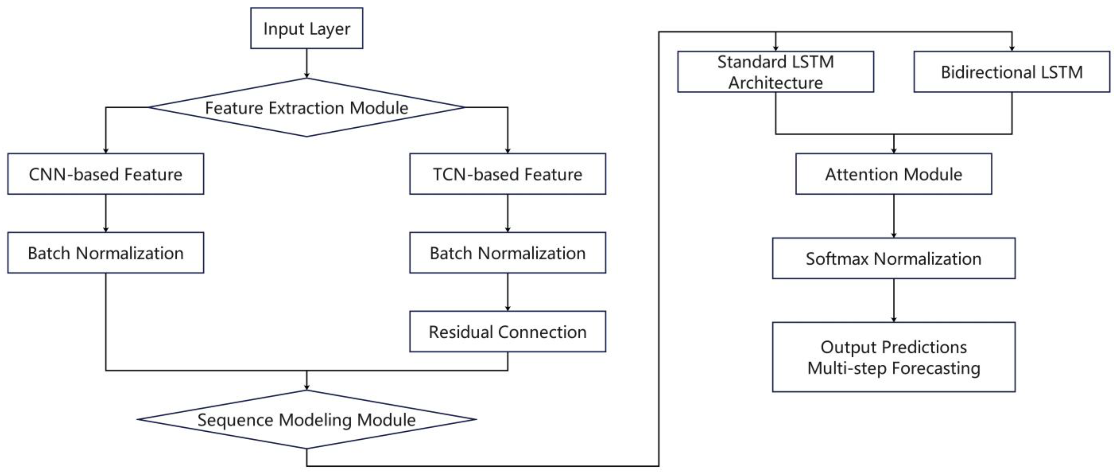
In this study, we developed four hybrid deep learning architectures to leverage the complementary strengths of different neural network structures. The CNN-LSTM-Attention model employs convolutional neural networks (CNNs) [28] to extract local temporal patterns, followed by Long Short-Term Memory (LSTM) [29] networks to capture long-term dependencies. An attention mechanism [30] highlights the most informative time steps. The CNN-BiLSTM-Attention model extends this design by incorporating bidirectional LSTM layers [31], enabling the capture of both forward and backward temporal dependencies. The TCN-LSTM-Attention model utilizes causal convolutions with dilations to ensure temporal causality while expanding the receptive field. This is combined with LSTM layers and an attention mechanism for enhanced predictive capability. Finally, the TCN-BiLSTM-Attention model integrates the long-sequence modeling capacity of Temporal Convolutional Networks (TCNs) with the bidirectional dependency learning of BiLSTM. This is further refined by attention to emphasize critical features and improve interpretability. Figure 1 illustrates the complete framework of the hybrid model.

2.1. Convolutional Neural Networks (CNN)

A CNN is a discriminative model architecture that excels in processing two-dimensional data with grid-like topologies, such as images and videos. Compared to traditional neural networks, CNNs demonstrate significant advantages in reducing computational latency. They employ a weight-sharing mechanism across the temporal dimension, effectively minimizing computational time consumption. Unlike traditional neural networks that utilize general matrix multiplication operations, CNNs substitute these with specialized convolution operations, thereby reducing model complexity by decreasing the number of parameters within the network [32].

A typical CNN architecture consists of an input layer, convolutional layers, pooling layers, fully connected layers, and an output layer. The input layer undergoes feature transformation and extraction through the convolutional and pooling layers. In the fully connected layers, local information from these layers is further integrated, mapping it to an output signal via the output layer [33], as shown in Figure 1.

Convolution layers are the core component of CNN architectures. Their unique feature lies in their partial connection approach, connecting only to a subset of neurons from the preceding layer. In addition, convolution kernel operations are utilized to extract key features from the input data. The formula is shown in (1).

$$l_t=\tanh \left(x_t\cdot k_t+b_t\right)$$

(1)

where l_t represents the output value after convolution, tanh is the activation function,  x_t is the input vector, k_t is the weight of the convolution kernel, and b_t is the bias of the convolution kernel.

The activation layer simulates the signal transmission mechanism of biological neurons by introducing nonlinear activation functions, enabling the network to solve complex nonlinear problems. Without activation functions, including common ones such as sigmoid, Tanh, and ReLU [34,35,36], deep networks would degenerate into linear models. Among these, the sigmoid function was the primary choice in early neural networks.

$$\mathrm{Sigmoid}(x)={\displaystyle \frac{1}{1+e^{-x}}}$$

(2)

Despite this, it suffers from the vanishing gradient problem (where gradients approach zero when far from zero), making model training difficult. Consequently, it has gradually been replaced by newer activation functions.

The Tanh function (tangent to the hyperbola) serves as an improved alternative; its formula is shown in (3).

$$\mathrm{Tanh}(x)={\displaystyle \frac{e^x+e^{-x}}{e^x-e^{-x}}}$$

(3)

This function is commonly used to generate model output activations, constraining its range to the interval (−1, 1).

ReLU (Rectified Linear Unit), as the current most common activation function, is defined by the formula shown in (4).

$$f(x)=\max (x,0)$$

(4)

The activation mechanism of the ReLU function is as follows: positive inputs pass through unchanged, while negative inputs yield an output of zero. After comprehensively comparing the characteristics of various activation functions and considering the requirements of this study, ReLU was ultimately selected as the network activation function.

2.2. Temporal Convolutional Network (TCN)

Temporal Convolutional Networks (TCNs), an enhanced structure based on convolutional neural networks (CNNs) proposed by Bai et al., exhibit outstanding memory capabilities [37]. They effectively capture temporal dependencies within sequence data and thus they are widely adopted for sequence-information-processing tasks. TCNs primarily consist of causal and dilated convolutional layers, residual connection structures, and normalization/activation units. Through multi-layer stacking, it progressively extracts and represents temporal features.

In time series modeling, the convolution formula is as follows:

$$y\left(t\right)={\displaystyle \sum _{i=0}^{k-1}{W}_i}\times x\left(t-i\right)$$

(5)

Here, y(t) is the output feature sequence, x(t) is the input time series, and W_i is the convolutional kernel weight of length k. To enable the model to capture long-term temporal dependencies, dilated convolutions are employed, where the formula is:

$$y\left(t\right)={\displaystyle \sum _{i=0}^{k-1}{W}_i}\cdot x\left(t-d\times i\right)$$

(6)

Here, d is the expansion factor, which determines how far back in time the current moment relates to historical data. Causal dilated convolution further ensures that x(t) depends solely on past data and is independent of future time series data. To prevent vanishing gradients, TCNs employ residual connections, with the overall formula shown below:

$$X\prime =ReLU\left\{BatchNorm[conv1D(X)]\right\}+X$$

(7)

where X is the output sequence from the TCN, BatchNorm is the normalized data to enhance training stability, and ReLU is the activation function. Residual connections preserve input information and prevent gradient vanishing.

Although CNNs were originally developed for two-dimensional data such as images, they have been successfully adapted to one-dimensional sequence forecasting tasks. In this study, a CNN is applied to extract local temporal dependencies from time series data by using one-dimensional convolutional filters.

2.3. Bidirectional Long Short-Term Memory (BiLSTM)

LSTM is an adaptive recurrent neural network (RNN) whose core structure consists of memory cells and gating mechanisms. Each neuron maintains an internal state through memory cells and regulates information flow via multiplicative gating units. An LSTM layer comprises multiple interconnected memory blocks, each containing one or more recursively linked memory cells. A standard LSTM cell features an input gate and an output gate: the input gate controls whether external data is written into the internal state, determining what information is retained or discarded; the output gate modulates the visibility of the internal state to external outputs [38]. LSTM units effectively capture range dependencies within input sequences. Their training algorithm is based on error gradient computation, integrating real-time recurrent learning with backpropagation mechanisms [39]. Unlike traditional RNNs, which suffer from the vanishing gradient problem, LSTM mitigates this issue through its gating mechanisms. Long-term dependencies are processed through memory blocks rather than solely relying on the backward propagation of error gradients, which allows LSTM to be effectively trained using backpropagation through time (BPTT). This enables LSTM to capture long-range dependencies in sequential data and achieve more stable performance compared with traditional RNNs [40].

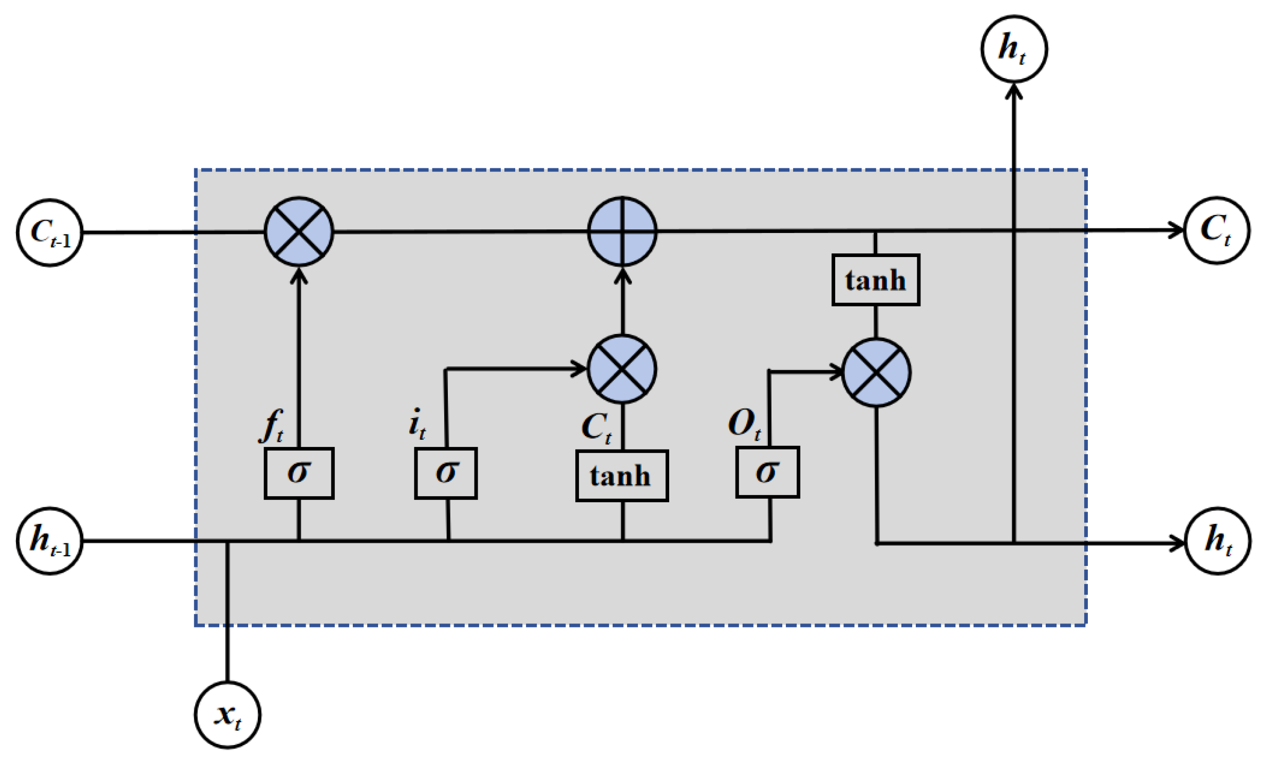
The core structure of LSTM comprises memory units and nonlinear gating mechanisms. The former maintain internal states across time steps, while the latter regulate the flow of information within the network [41]. From a secure network perspective, LSTM neurons consist of both internal and external components. Therefore, attention should not be focused solely on the neuron’s output but also on its internal structure. The schematic diagram is shown in Figure 2.

Mathematically, the LSTM unit is defined as:

$$f_t=\sigma \left(W_f\cdot \left[h_{(t-1)},x_t\right]+b_f\right)$$

(8)

$$i_t=\sigma \left(W_i\cdot \left[h_{(t-1)},x_t\right]+b_i\right)$$

(9)

$$C_r=f_e\cdot C_e+i_e\cdot \tanh \left(W_e\cdot [h_e,v_e]+b_e\right)$$

(10)

$$O_t=\sigma \left(W_o\cdot [h_{t-1},a_t]+b_o\right)$$

(11)

$$h_t=o_t\cdot \tanh \left(C_t\right)$$

(12)

Among these, Formula (8) is the forget gate, Formula (9) is the input gate, Formula (10) is the cell state, Formula (11) is the output gate, Formula (12) is the hidden state, σ is the sigmoid function, ‘·’ is the dot product, [h_(t−1), x_t] is the concatenation of the previous hidden state and the current input, and ‘W’ and ‘b’ are the weight and bias parameters, respectively.

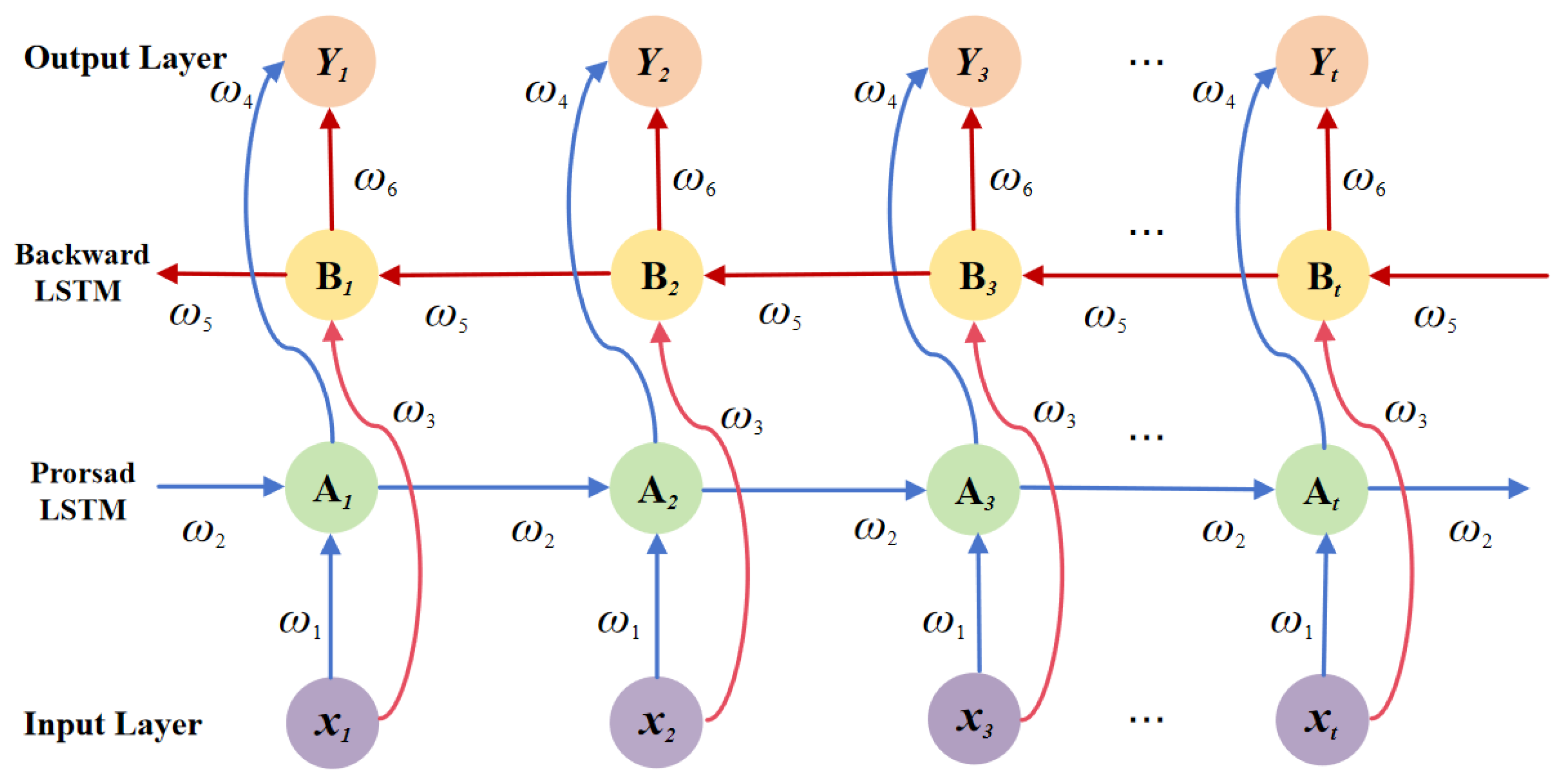
The Bidirectional Long Short-Term Memory (BiLSTM) neural network is an optimized refinement of the LSTM [42]. Traditional LSTM models predict current outputs using past temporal information, whereas BiLSTM has enhanced sequence modeling capabilities and an improved model robustness through simultaneous integration of historical and future contextual information through the combination of forward and backward LSTM layers [43]. The working principle is shown in Figure 3.

The sequence modeling capabilities of BiLSTM are effectively enhanced by integrating forward and backward LSTM units. This specialized architecture not only resolves the gradient vanishing problem in traditional RNNs but also simultaneously captures bidirectional long-term dependency features. Its forward propagation process can be expressed as:

$$h_l^{(1)}=f(u^{(1)}{h}_{l-1}^{(1)}+w^{(1)}{x}_l+b^{(1)})$$

(13)

$$h_l^{(2)}=f(u^{(2)}{h}_{l-1}^{(2)}+w^{(2)}{x}_l+b^{(2)})$$

(14)

The final hidden layer output is the concatenation of the outputs from the first two layers’ opposite neurons:

$$y_t=g\left(u\left[h^{(1)};h^{(2)}\right]+c\right)$$

(15)

Here, f(·) denotes the activation function employed and $h_t^{\left(1\right)}$ represents the output of the forward LSTM, while $h_t^{\left(2\right)}$ denotes the output of the backward LSTM. Here, U(i), W(i), and b(i) (i = 1, 2), respectively, denote the weight matrices and bias vectors.

BiLSTM can better process sequential data by utilizing bidirectional information, thereby improving model accuracy.

2.4. Attention

Attention mechanisms were initially inspired by the human visual system. Unlike traditional neural networks that struggle to distinguish information importance, this mechanism assigns differential weights to input features—enhancing key information while suppressing redundant content. This approach improves the information processing efficiency and mitigates potential information loss in modeling long sequences, such as within LSTM networks. Consequently, incorporating attention mechanisms holds promise for further enhancing the accuracy of gas price predictions.

The core concept of the attention mechanism is the calculation of an attention score for each element in the input sequence, then assigning a weight to each element. This weight reflects the importance of each input element to the current task. The final output is the weighted sum of the input elements, highlighting the most relevant information. Specifically, assume the input matrix is X. By applying linear transformations to X, we obtain the query Q(Query), key K(Key), and value V(Value) matrices. Then, a scoring function is selected to compute the correlation scores between each element of the query and key matrices. These scores are subsequently converted into a probability distribution via the softmax function to derive the weights W; the formula is shown in (16).

$$W=\mathrm{s}\mathrm{o}\mathrm{f}\mathrm{t}\mathrm{m}\mathrm{a}\mathrm{x}\left(\mathrm{s}\mathrm{c}\mathrm{o}\mathrm{r}\mathrm{e}\right(Q,K\left)\right)$$

(16)

In this formula, ‘score’ represents the scoring function. Common scoring functions include the point-product model, the scaled point-product model, and the additive model. The formula is shown in (17) to (19).

$$\mathrm{s}\mathrm{c}\mathrm{o}\mathrm{r}\mathrm{e}(Q,K)=Q{K}^T$$

(17)

$$\mathrm{s}\mathrm{c}\mathrm{o}\mathrm{r}\mathrm{e}(Q,K)={\displaystyle \frac{Q{K}^T}{\sqrt{d_k}}}$$

(18)

$$\mathrm{s}\mathrm{c}\mathrm{o}\mathrm{r}\mathrm{e}(Q,K)=W_v^T\mathrm{t}\mathrm{a}\mathrm{n}\mathrm{h}(W_{k}K+W_{q}Q)$$

(19)

Here, $d_k$ denotes the key vector dimension and $\sqrt{d_k}$ serves as the scaling factor to prevent excessively large dot product values and mitigate the vanishing gradient problem, while W_v, W_q, and W_k are learnable parameters. Finally, the attention weights are multiplied by the value matrix to generate the final output O of the attention mechanism; the formula is shown in (20).

$$O=WV$$

(20)

2.5. Selection and Description of Research Data

With the increasing marketization of natural gas prices, trading hubs have assumed a more critical role in facilitating the flow and allocation of global natural gas resources. Among the three major regional hubs worldwide, the Henry Hub in the United States stands out as the most liquid and influential [44]. The dataset employed in this study was obtained from the U.S. 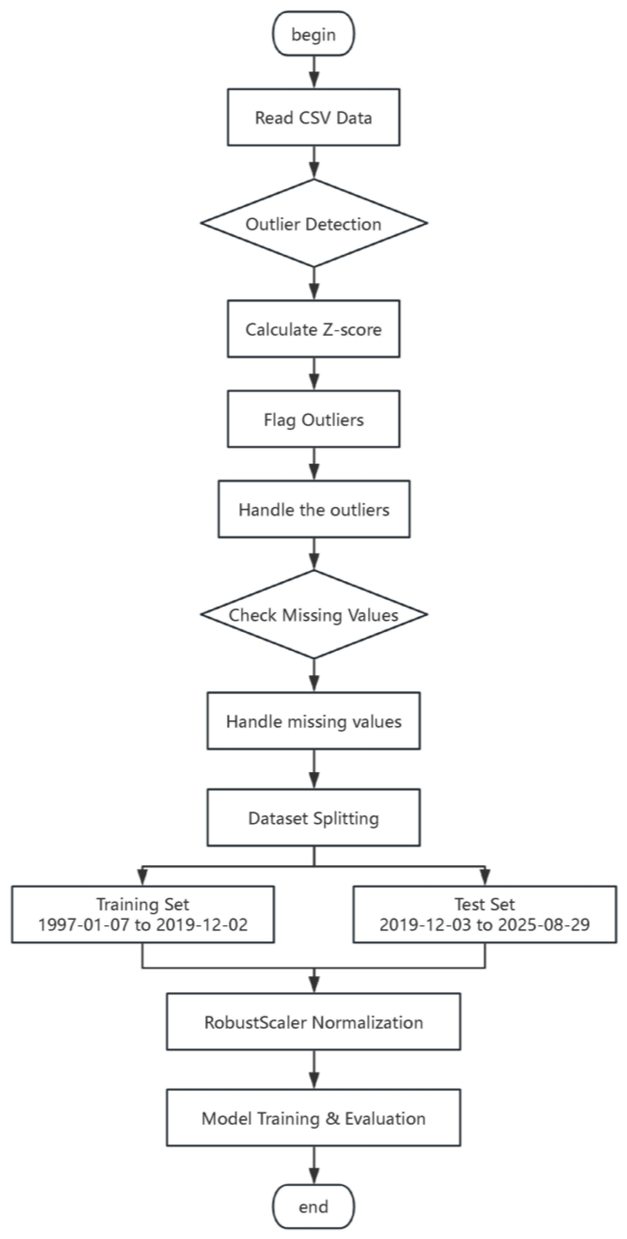Energy Information Administration (https://www.eia.gov, accessed on 30 August 2025); additional data description is provided in the Supplementary Materials. The data span a long historical period, with the training set covering 7 January 1997, to 2 December 2019, comprising 5760 observations, and the testing set covering 3 December 2019, to 29 August 2025, comprising 1439 observations. This division ensures that the models are trained on sufficient historical information while being evaluated on a more recent period to assess their predictive performance.

To ensure the reproducibility of the experiments, the settings of the key hyperparameters for all hybrid deep learning models are summarized in

Table 1. Hyperparameter Settings for Hybrid Deep Learning Models.

Component	Parameter/Setting	Value/Description
Lookback window	lookback	9
Forecasting horizon	horizon	1, 2, 3, 4 steps ahead
Convolutional layer	type/filters/kernel/activation	1D-CNN, 32 filters, kernel size = 3, ReLU activation
LSTM/BiLSTM layers	units/return_sequences	64 units (first layer, return_sequences=True), 32 units (second LSTM layer)
Attention mechanism	dense activation/softmax/multiplication	Dense with tanh, softmax normalization, elementwise multiplication with LSTM output
Optimizer	type/learning rate	Adam, lr = 0.001
Loss function		Mean Squared Error (MSE)
Batch size		32
Epochs		20
Output layer	activation	Linear

. These settings include the lookback window size, forecasting horizons, convolutional layer configuration, LSTM/BiLSTM units, attention mechanism design, optimizer, loss function, batch size, and number of training epochs. By explicitly reporting these parameters, readers can replicate the model architectures and training procedures, thereby validating the experimental results presented in this study. The data flow diagram is shown in Figure 4.

2.6. Evaluation Metrics

With regard to performance evaluation, the choice of evaluation metrics in this study is motivated by their complementary ability to assess forecasting performance from different perspectives. The mean absolute error (MAE), root mean squared error (RMSE), mean absolute percentage error (MAPE), and coefficient of determination (R²) were employed. The MAE and RMSE are widely used in regression tasks as they quantify absolute and squared deviations between predictions and observations, with the RMSE being more sensitive to large errors. The MAPE provides a scale-independent measure by expressing errors in relative percentage terms, which facilitates comparability across different datasets and time periods. R², on the other hand, measures the proportion of variance explained by the model, offering an interpretable indicator of the overall goodness-of-fit. Together, these four metrics provide a balanced and comprehensive evaluation of both accuracy and explanatory power, thereby ensuring robustness in performance assessments.

Specifically, the four metrics are defined as follows:

$$\mathrm{MAPE}={\displaystyle \frac{1}{n}}{\displaystyle \sum _{i=1}^n\left|\frac{y_i-{\widehat{y}}_i}{y_i}\right|}\times 100\%$$

(21)

$$\mathrm{MAE}={\displaystyle \frac{1}{n}}{\displaystyle \sum _{i=1}^n}|y_i-{\widehat{y}}_i|$$

(22)

$$\mathrm{RMSE}=\sqrt{{\displaystyle \frac{1}{n}}{\displaystyle \sum _{i=1}^n{(y_i-{\widehat{y}}_i)}^2}}$$

(23)

$$R^2=1-{\displaystyle \frac{{\displaystyle \sum _{i=1}^n{(y_i-{\widehat{y}}_i)}^2}}{{\displaystyle \sum _{i=1}^n{(y_i-\overline{y})}^2}}}$$

(24)

2.7. Hybrid Deep Learning Architectures

To exploit the complementary strengths of convolutional, recurrent, and attention-based models, this study explores four hybrid deep learning architectures: CNN-LSTM-Attention, CNN-BiLSTM-Attention, TCN-LSTM-Attention, and TCN-BiLSTM-Attention. Each model integrates different neural components to enhance temporal feature extraction, long-term dependency modeling, and interpretability.

CNN-LSTM-Attention. In this architecture, one-dimensional convolutional layers are first applied to extract local temporal patterns from natural gas price sequences. CNN filters capture short-term fluctuations and reduce noise by emphasizing key subsequences. The extracted features are then fed into LSTM layers, which model long-term temporal dependencies by leveraging gated memory cells. Finally, an attention mechanism is introduced to assign adaptive weights to different time steps, allowing the model to prioritize the most influential historical information for prediction.

CNN-BiLSTM-Attention. While a CNN and LSTM provide strong local and sequential modeling capabilities, the unidirectional nature of LSTM limits its ability to incorporate future context. The CNN-BiLSTM-Attention model addresses this limitation by replacing LSTM with bidirectional LSTM layers, which process the input sequence in both forward and backward directions. This design enables the model to capture dependencies from both past and future observations. The attention mechanism further enhances interpretability by emphasizing the most relevant bidirectional features in the forecasting task.

TCN-LSTM-Attention. Temporal Convolutional Networks (TCNs) offer efficient long-sequence modeling through dilated causal convolutions and residual connections. In this hybrid design, TCN layers are employed to ensure temporal causality while expanding the receptive field, thereby capturing multi-scale dependencies within the input series. The extracted features are subsequently passed into LSTM layers for refined long-term dependency modeling. The attention module adaptively highlights critical time steps, improving both predictive accuracy and interpretability.

TCN-BiLSTM-Attention. The final hybrid framework integrates the strengths of a TCN and BiLSTM. TCN layers first extract hierarchical temporal features under the constraint of causality, while BiLSTM layers complement this by learning bidirectional contextual dependencies that the TCN alone cannot capture. The attention mechanism then adaptively selects and emphasizes the most important temporal representations. This comprehensive integration enhances the model’s robustness, interpretability, and ability to generalize across varying market conditions.

3. Results

To evaluate the predictive performance of the proposed hybrid models, we conducted experiments under different forecasting horizons with a fixed lookback window of 9. The results are summarized in

Table 2. Performance comparison of different hybrid models with lookback = 9 under multi-step forecasting.

Lookback	Horizon	Model	MAE	RMSE	MAPE(%)	R2
9	1	CNN-LSTM-Attention	0.193	0.377	5.58	95.75%
9	1	CNN-BiLSTM-Attention	0.177	0.370	5.05	95.89%
9	1	TCN-LSTM-Attention	0.180	0.373	5.04	95.84%
9	1	TCN-BiLSTM-Attention	0.190	0.381	5.63	95.66%
9	2	CNN-LSTM-Attention	0.217	0.435	6.35	94.35%
9	2	CNN-BiLSTM-Attention	0.221	0.450	6.27	93.95%
9	2	TCN-LSTM-Attention	0.236	0.450	7.21	93.94%
9	2	TCN-BiLSTM-Attention	0.223	0.443	6.35	94.13%
9	3	CNN-LSTM-Attention	0.257	0.491	7.67	92.77%
9	3	CNN-BiLSTM-Attention	0.250	0.510	7.10	92.23%
9	3	TCN-LSTM-Attention	0.254	0.487	7.39	92.89%
9	3	TCN-BiLSTM-Attention	0.258	0.503	7.35	92.43%
9	4	CNN-LSTM-Attention	0.268	0.518	7.71	91.96%
9	4	CNN-BiLSTM-Attention	0.267	0.533	7.53	91.50%
9	4	TCN-LSTM-Attention	0.282	0.526	8.35	91.73%
9	4	TCN-BiLSTM-Attention	0.272	0.534	7.70	91.48%

, and Figure 5 illustrates the prediction curves for a visual comparison between models.

The results reveal that with a forecasting horizon of one step (T + 1), all four models achieve high predictive accuracies, with all R² values exceeding 95%. CNN-BiLSTM-Attention and TCN-LSTM-Attention exhibit slightly better performance, with MAE values of 0.177 and 0.180, respectively, an MAPE of around 5.0%, and an R² above 95.8%. As the forecasting horizon increases from 2 to 4 steps, errors gradually increase, and the explanatory power decreases, with R² declining to around 91%. This confirms the inherent challenge of long-term forecasting. Notably, CNN-BiLSTM-Attention maintains a relatively stable performance, suggesting stronger robustness under extended horizons.

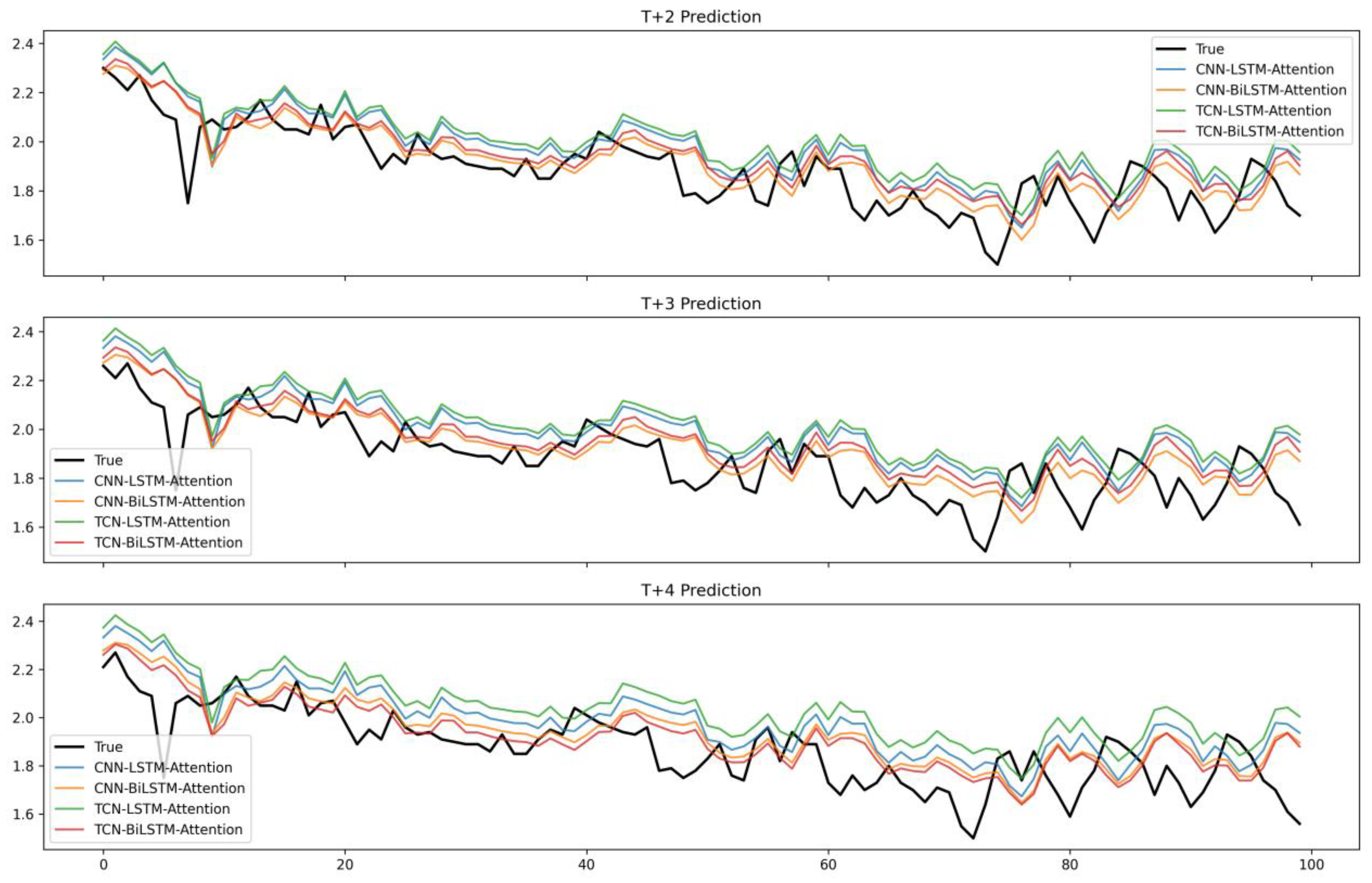
The predictive trajectories of the models are illustrated in Figure 5 (one-step forecasting) and Figure 6 (multi-step forecasting). In the one-step prediction task (Figure 5), all models successfully capture the overall dynamics of the target series. The CNN-BiLSTM-Attention and TCN-LSTM-Attention models produce predictions that closely follow the ground truth, particularly in periods with sharp fluctuations. In the multi-step forecasting scenarios (Figure 6), prediction errors accumulate as the horizon lengthens, leading to visible deviations from the true values. However, CNN-BiLSTM-Attention consistently demonstrates smaller divergence, thereby validating its stability in longer-horizon predictions.

Overall, the comparative experiments demonstrate that all four hybrid architectures, combining convolutional, recurrent, and attention mechanisms, achieve satisfactory forecasting performances, with R² values remaining above 91% across all tested horizons. Short-term forecasts benefit from the synergy of CNN feature extraction, LSTM/BiLSTM sequential learning, and attention-based refinement.

However, in the context of energy commodity forecasting, the cumulative effect of multi-step prediction errors warrants particular attention. Natural gas markets are characterized by high volatility, mean reversion, and susceptibility to external shocks. As the forecast horizon increases, even minor errors in preceding steps can propagate and be amplified, leading to significant deviations in later predictions. This poses substantial challenges for practical applications, outline in the following:

Trading and Portfolio Management: Inaccurate multi-step forecasts can lead to suboptimal hedging decisions or timing errors in futures contracts, directly impacting profitability.

Infrastructure and Storage Operation: For utilities and storage operators, forecasts over multiple periods are crucial for scheduling. Error accumulation could result in costly physical imbalances, such as under-supply during demand spikes or overpaying for storage injections.

Risk Assessment: The tail risk of natural gas prices is a critical concern. Models that poorly manage error accumulation may underestimate the Value-at-Risk (VaR) during turbulent market periods, exposing firms to unforeseen financial losses.

Among the tested models, CNN-BiLSTM-Attention provides the most favorable balance between accuracy and robustness. Crucially, its bidirectional learning capability and the attention mechanism allow it to more effectively capture long-range dependencies and dynamically weigh the importance of past market states. This enables the model not only to achieve high single-step accuracy but also to mitigate the propagation of errors across subsequent forecasting steps, thereby delivering a more reliable performance over longer horizons. This characteristic makes it a particularly promising candidate for practical deployment in energy markets, where dependable multi-step forecasts are essential for sequential decision-making.

4. Robustness Test

4.1. The Various Forecasting Time Frames

To validate the stability of the proposed natural gas price prediction models across different time horizons, the prediction steps were expanded to T + 5, T + 6, T + 7, and T + 8 ahead, and a comparative evaluation of the proposed hybrid models was conducted using four key metrics: MAE, RMSE, MAPE, and R².

Table 3. Performance comparison of different hybrid models with lookback = 9 under multi-step forecasting horizons.

Lookback	Horizon	Model	MAE	RMSE	MAPE (%)	R2
9	5	CNN-LSTM-Attention	0.290	0.555	8.21	90.79%
9	5	CNN-BiLSTM-Attention	0.298	0.571	8.48	90.25%
9	5	TCN-LSTM-Attention	0.297	0.561	8.49	90.58%
9	5	TCN-BiLSTM-Attention	0.293	0.563	8.26	90.51%
9	6	CNN-LSTM-Attention	0.301	0.572	8.41	90.24%
9	6	CNN-BiLSTM-Attention	0.309	0.587	8.73	89.69%
9	6	TCN-LSTM-Attention	0.309	0.576	8.89	90.10%
9	6	TCN-BiLSTM-Attention	0.313	0.589	8.71	89.62%
9	7	CNN-LSTM-Attention	0.325	0.607	9.31	89.01%
9	7	CNN-BiLSTM-Attention	0.326	0.625	9.21	88.34%
9	7	TCN-LSTM-Attention	0.339	0.604	10.00	89.12%
9	7	TCN-BiLSTM-Attention	0.333	0.631	9.27	88.12%
9	8	CNN-LSTM-Attention	0.341	0.622	9.96	88.43%
9	8	CNN-BiLSTM-Attention	0.343	0.648	9.71	87.47%
9	8	TCN-LSTM-Attention	0.344	0.635	9.65	87.98%
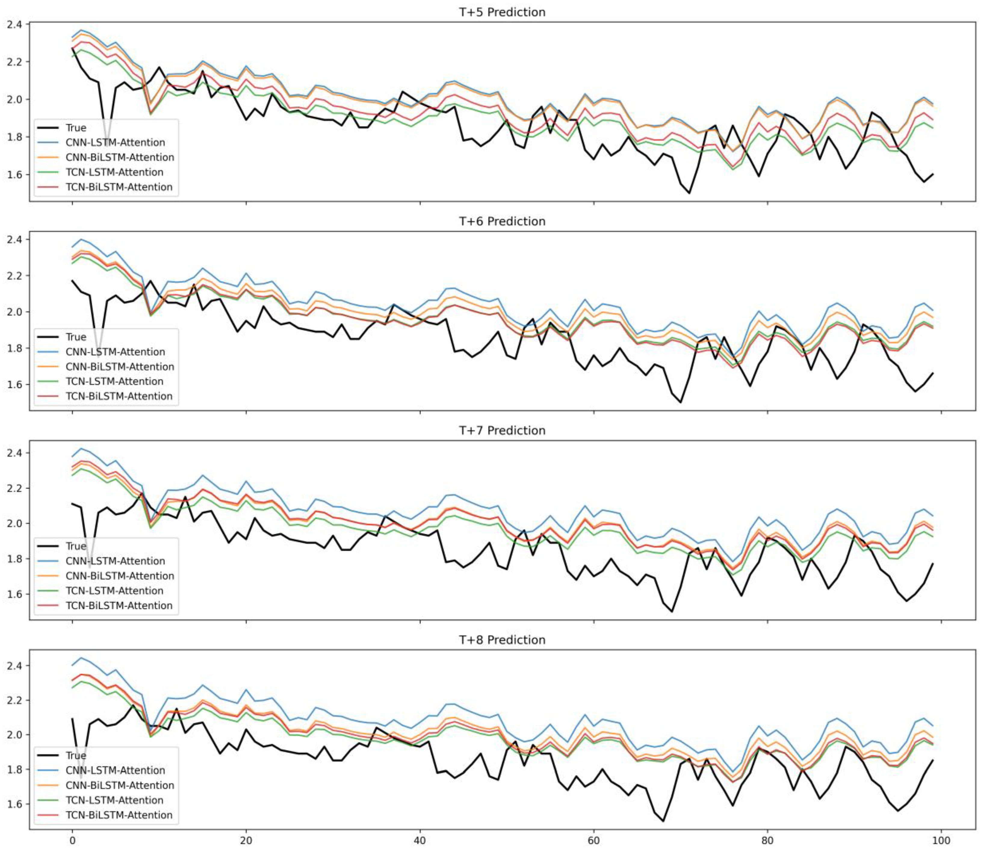
9	8	TCN-BiLSTM-Attention	0.340	0.640	9.51	87.76%

reports the quantitative forecasting results of the four hybrid deep learning models with a lookback window of 9 and prediction horizons ranging from T + 5 to T + 8, while Figure 7 presents the corresponding prediction curves. It can be observed that all models achieve a competitive short-term prediction accuracy, with MAE values between 0.290 and 0.344, RMSEs ranging from 0.555 to 0.648, and MAPEs within 8.21–10.00%. The R² values remain above 87% across all horizons, indicating a strong explanatory power and stable generalization capability. Notably, at horizon T + 5, the CNN–LSTM–Attention model achieves the lowest MAE (0.290) and MAPE (8.21%), demonstrating its superior precision in short-term forecasting. However, as the prediction horizon extends to T + 8, all models exhibit a gradual performance degradation, reflected in increased MAE, RMSE, and MAPE values, together with declining R² scores. This phenomenon highlights the typical challenge of multi-step time series forecasting—the accumulation of error propagation as the prediction horizon increases. From the visual inspection of Figure 7, the predicted curves of CNN–LSTM–Attention and TCN–BiLSTM–Attention show closer alignment with the ground truth compared with the other two models, particularly for local fluctuations. These findings suggest that in hybrid architectures integrating convolutional or temporal convolutional feature extraction with attention-enhanced recurrent learning, robustness can be effectively improved and accuracy can be maintained under extended forecasting horizons.

4.2. Alternative Indicators for Gas Prices

Table 4. Forecasting performance of hybrid deep learning models on the NYMEX dataset across different horizons.

Lookback	Horizon	Model	MAE	RMSE	MAPE (%)	R2
9	1	CNN-LSTM-Attention	0.112	0.176	3.22	98.80%
9	1	CNN-BiLSTM-Attention	0.116	0.181	3.29	98.73%
9	1	TCN-LSTM-Attention	0.112	0.176	3.17	98.80%
9	1	TCN-BiLSTM-Attention	0.116	0.184	3.29	98.69%
9	2	CNN-LSTM-Attention	0.137	0.222	3.81	98.09%
9	2	CNN-BiLSTM-Attention	0.136	0.213	3.91	98.25%
9	2	TCN-LSTM-Attention	0.132	0.209	3.78	98.31%
9	2	TCN-BiLSTM-Attention	0.134	0.212	3.80	98.27%
9	3	CNN-LSTM-Attention	0.165	0.266	4.47	97.26%
9	3	CNN-BiLSTM-Attention	0.150	0.240	4.27	97.78%
9	3	TCN-LSTM-Attention	0.162	0.252	4.51	97.54%
9	3	TCN-BiLSTM-Attention	0.158	0.246	4.50	97.66%
9	4	CNN-LSTM-Attention	0.168	0.268	4.80	97.22%
9	4	CNN-BiLSTM-Attention	0.169	0.268	4.77	97.22%
9	4	TCN-LSTM-Attention	0.166	0.265	4.70	97.28%
9	4	TCN-BiLSTM-Attention	0.168	0.267	4.78	97.24%

presents the forecasting performance of the four hybrid models (CNN–LSTM–Attention, CNN–BiLSTM–Attention, TCN–LSTM–Attention, and TCN–BiLSTM–Attention) on the NYMEX dataset. The training period spans from 3 April 1990, to 23 April 2018, and the testing set covers 24 April 2018, to 17 June 2025. When the lookback window is 9, the results indicate that all models achieve highly accurate short-term forecasts. For one-step-ahead prediction (horizon = 1), the MAE remains low at 0.112–0.116, the RMSE is around 0.176–0.184, the MAPE is close to 3.2%, and the R² is above 98.6%, confirming the models’ excellent fitting capability and robustness. As the horizon extends, a gradual degradation in accuracy is observed: at horizon = 2, the MAE rises to 0.132–0.137 and R² decreases slightly to ~98.1–98.3%, while at horizon = 3–4, the MAE further increases to 0.150–0.169 and the R² decreases to ~97.2–97.8%. This trend reflects the inevitable error accumulation in multi-step forecasting.

In terms of model comparison, CNN–LSTM–Attention and TCN–LSTM–Attention achieve the lowest MAE (0.112) at horizon = 1, while TCN–LSTM–Attention performs best at horizon = 2 (MAE = 0.132, RMSE = 0.209, MAPE = 3.78%). At longer horizons (T + 3 and T + 4), CNN-BiLSTM–Attention and TCN–BiLSTM–Attention demonstrate more stable performances relatively, suggesting that bidirectional recurrent structures combined with attention mechanisms are better at mitigating information loss in extended forecasts. Overall, the results highlight that all four hybrid models maintain a high predictive power on the NYMEX dataset, with CNN–LSTM–Attention excelling in very short-term forecasts and TCN-based variants showing advantages in capturing temporal dependencies under longer horizons. 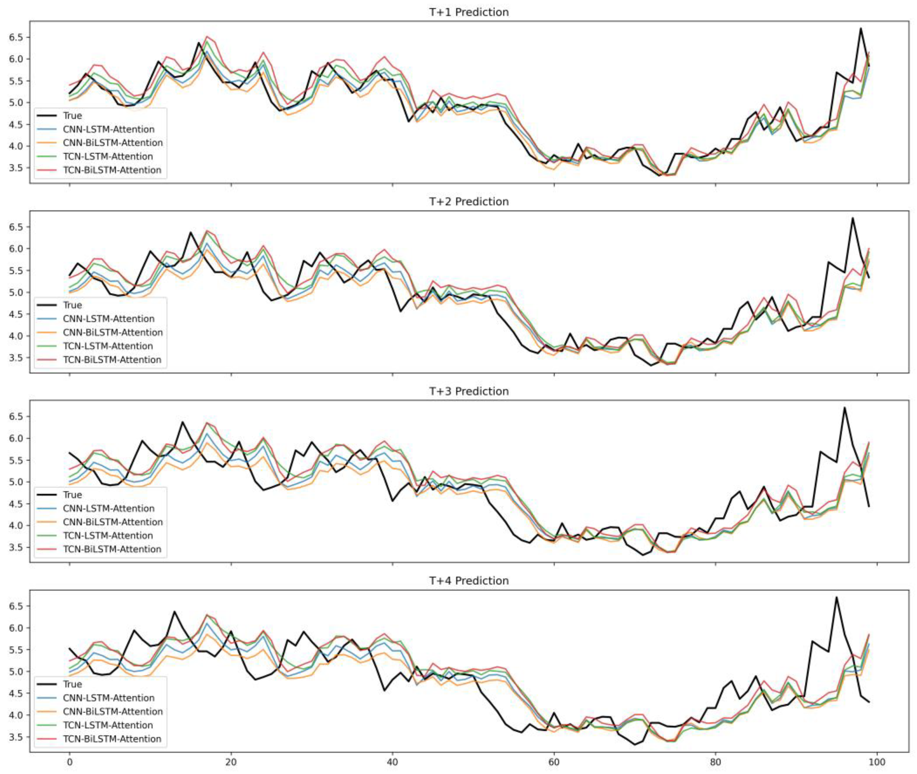As shown in Figure 8, based on NYMEX natural gas price data, the CNN-LSTM-Attention, CNN-BiLSTM-Attention, TCN-LSTM-Attention, and TCN-BiLSTM-Attention models exhibit strong capability in tracking the price dynamics across multi-step forecasts.

4.3. A Comparative Analysis of the Prognostication Horizon Dimensions

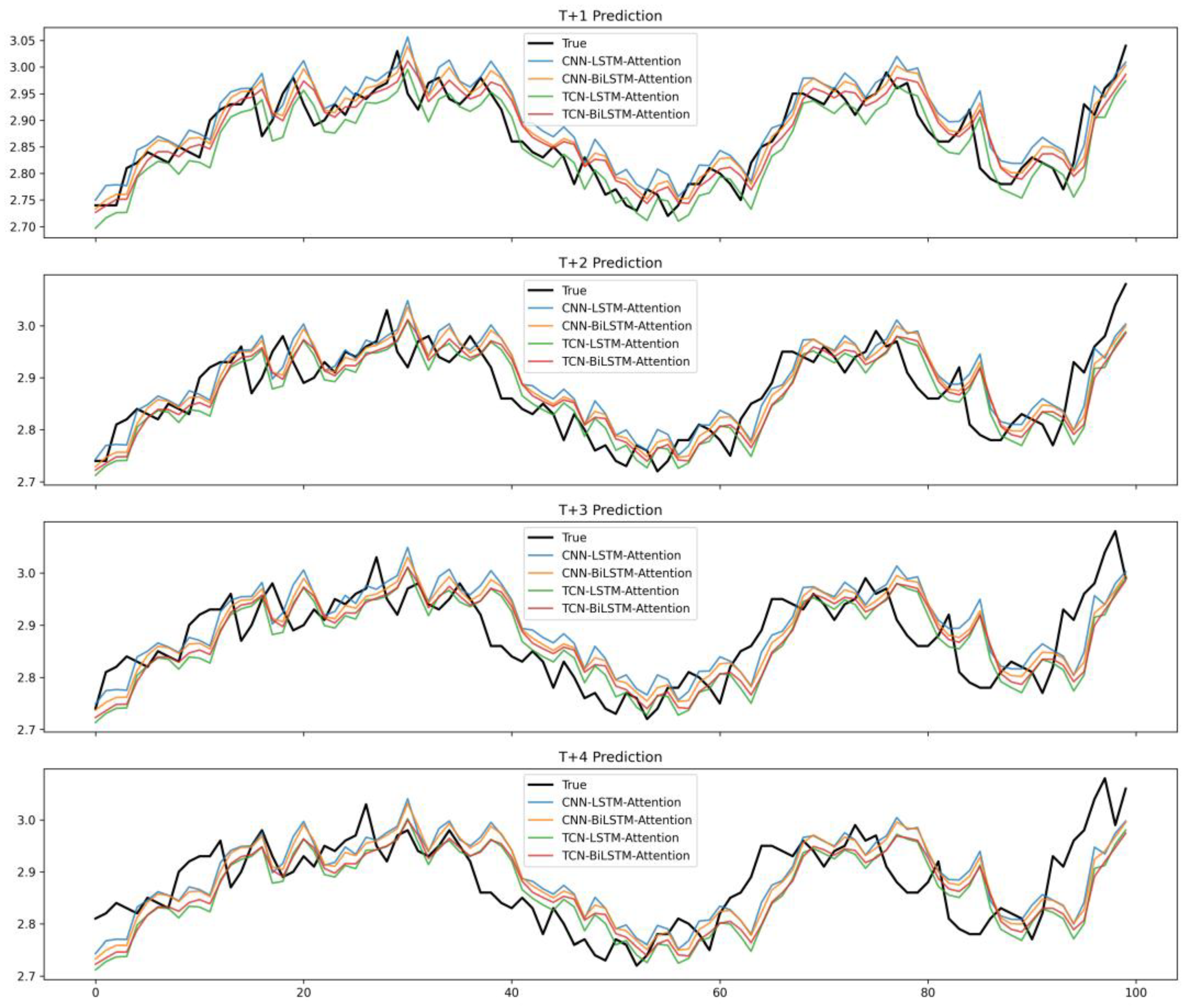
In this study, a sliding window approach is employed to tackle a time series prediction task, and an empirical analysis is conducted based on the association between temporal partitioning of historical data and model performance step size. In terms of data partitioning, the training set covers 3979 samples from 1 December 2005, to 27 August 2021, and is used for model parameter learning and fitting, while the test set consists of 1002 samples from 30 August 2021, to 29 August 2025, and was specifically selected to evaluate the model’s out-of-sample prediction capability, ensuring the objectivity and generalizability of the validation results.

Rossi and Inoue (2012) emphasized that the definition of prediction horizons and evaluation windows can substantially affect out-of-sample forecasting outcomes, highlighting the importance of careful horizon selection in empirical analysis [45]. Consistent with this argument, the results reported in

Table 5. Forecasting performance of hybrid deep learning models on the dataset with a lookback window of 9 (2005–2025).

Lookback	Horizon	Model	MAE	RMSE	MAPE (%)	R2
9	1	CNN-LSTM-Attention	0.203	0.358	5.53	96.73%
9	1	CNN-BiLSTM-Attention	0.223	0.397	5.80	95.97%
9	1	TCN-LSTM-Attention	0.202	0.364	5.40	96.62%
9	1	TCN-BiLSTM-Attention	0.217	0.384	5.77	96.24%
9	2	CNN-LSTM-Attention	0.239	0.410	6.36	95.70%
9	2	CNN-BiLSTM-Attention	0.242	0.430	6.44	95.27%
9	2	TCN-LSTM-Attention	0.243	0.415	6.41	95.61%
9	2	TCN-BiLSTM-Attention	0.251	0.427	6.85	95.35%
9	3	CNN-LSTM-Attention	0.279	0.459	7.23	94.61%
9	3	CNN-BiLSTM-Attention	0.286	0.477	7.68	94.19%
9	3	TCN-LSTM-Attention	0.289	0.458	8.24	94.64%
9	3	TCN-BiLSTM-Attention	0.277	0.464	7.25	94.50%
9	4	CNN-LSTM-Attention	0.302	0.494	7.83	93.76%
9	4	CNN-BiLSTM-Attention	0.334	0.521	9.16	93.07%
9	4	TCN-LSTM-Attention	0.301	0.493	7.99	93.80%
9	4	TCN-BiLSTM-Attention	0.313	0.511	8.27	93.33%

reveal a clear pattern: while all four hybrid models (CNN–LSTM–Attention, CNN–BiLSTM–Attention, TCN–LSTM–Attention, and TCN–BiLSTM–Attention) achieve high accuracy at the one-step-ahead horizon (MAE ≈ 0.202–0.223, R² ≈ 96–97%), the forecasting errors gradually accumulate as the horizon extends to T + 4, with MAE rising to 0.301–0.334 and R² declining to 93–94%. This degradation underscores the inherent trade-off between horizon length and prediction reliability, reinforcing the necessity of horizon-sensitive evaluation strategies in practical forecasting applications. Figure 9 illustrates the multi-step ahead forecasting performance (horizons = 1–4) of the proposed models over the full study period (2005–2025).

4.4. A Comparative Analysis of Forecasting Models

To comprehensively assess the multi-step ahead forecasting performance, we first analyzed the graphical and tabular results. As depicted in the multi-panel figure, the prediction curves of different models exhibit varying degrees of deviation from the true values as the forecasting horizon extends from T + 1 to T + 4. Quantitatively, the evaluation metrics (MAE, RMSE, MAPE, R²) across all horizons and models further elucidate the performance trends.

While single-component models like CNN and LSTM can achieve reasonable results at shorter horizons (e.g., T + 1 MAE of 0.2546 for CNN and 0.1866 for LSTM), their performance deteriorates noticeably with an increasing horizon length. For instance, the MAE of the CNN rises from 0.2546 at T + 1 to 0.3679 at T + 4, and the R² drops from 0.9293 to 0.8646. This highlights the inherent limitations of single-component models in capturing the complex, long-range dependencies and multi-scale patterns inherent in time series data.

In contrast, hybrid models (e.g., CNN—LSTM—Attention, CNN—BiLSTM—Attention, TCN—LSTM—Attention, TCN—BiLSTM—Attention) demonstrate superior and more robust performance across all forecasting horizons. Taking the T + 4 horizon as an example, the MAE of CNN—LSTM—Attention is 0.3383, which is notably lower than that of the single CNN model (0.3679) and even that of the single LSTM model (0.3415). The R² value of 0.8783 for CNN—LSTM—Attention at T + 4 is also better than that of both the CNN (0.8646) and LSTM (0.867).

The rationale for employing hybrid models, even when standard CNN or LSTM models can yield acceptable short-term predictions, lies in their ability to synergistically leverage the strengths of multiple architectural paradigms. CNNs excel at extracting local spatial or temporal features, and LSTMs (and BiLSTMs) are proficient in capturing sequential dependencies, while TCNs are efficient at handling long-range dependencies via dilated convolutions and attention mechanisms enable the model to focus on salient temporal segments. By combining these components, hybrid models can better address the multifaceted characteristics of time series—such as their non-stationarity, long-term memory effects, and intricate pattern interactions—that single-component models struggle to capture comprehensively. This architectural complexity is thus justified by the need to achieve higher accuracies, stronger generalization, and a more stable performance across different forecasting horizons, especially as the prediction task becomes more challenging with longer time lags. Figure 10 illustrates the multi-step ahead forecasting performance (horizons = 1–4) of the proposed models over the full study period.

Table 6. Evaluation of various forecasting models against an alternative benchmark.

Lookback	Horizon	Model	MAE	RMSE	MAPE (%)	R2
9	1	CNN-LSTM-Attention	0.189	0.381	5.51	95.66%
9	1	CNN-BiLSTM-Attention	0.176	0.370	4.98	95.90%
9	1	TCN-LSTM-Attention	0.181	0.375	5.20	95.78%
9	1	TCN-BiLSTM-Attention	0.185	0.374	5.43	95.81%
9	1	CNN	0.2546	0.4862	7.426	92.93%
9	1	BiLSTM	0.1798	0.3747	5.105	95.80%
9	1	LSTM	0.1866	0.3799	5.424	95.68%
9	1	TCN	0.2968	0.5558	8.366	90.76%
9	1	MovingAverage	0.307	0.579	8.60	89.96%
9	2	CNN-LSTM-Attention	0.235	0.440	7.29	94.20%
9	2	CNN-BiLSTM-Attention	0.213	0.435	6.00	94.32%
9	2	TCN-LSTM-Attention	0.218	0.435	6.17	94.33%
9	2	TCN-BiLSTM-Attention	0.229	0.459	6.49	93.69%
9	2	CNN	0.301	0.5624	8.676	90.54%
9	2	BiLSTM	0.2574	0.5043	7.217	92.39%
9	2	LSTM	0.2626	0.5132	7.559	92.12%
9	2	TCN	0.3333	0.6143	9.362	88.71%
9	2	MovingAverage	0.326	0.609	9.11	88.89%
9	3	CNN-LSTM-Attention	0.257	0.499	7.57	92.55%
9	3	CNN-BiLSTM-Attention	0.260	0.512	7.07	92.16%
9	3	TCN-LSTM-Attention	0.250	0.484	7.16	92.99%
9	3	TCN-BiLSTM-Attention	0.252	0.500	7.17	92.51%
9	3	CNN	0.3369	0.627	9.505	88.24%
9	3	BiLSTM	0.3062	0.6011	8.556	89.19%
9	3	LSTM	0.3107	0.6093	8.816	88.89%
9	3	TCN	0.3706	0.6736	10.472	86.42%
9	3	MovingAverage	0.342	0.635	9.56	87.92%
9	4	CNN-LSTM-Attention	0.270	0.527	7.65	91.70%
9	4	CNN-BiLSTM-Attention	0.277	0.548	7.68	91.01%
9	4	TCN-LSTM-Attention	0.273	0.526	7.69	91.71%
9	4	TCN-BiLSTM-Attention	0.292	0.557	8.67	90.71%
9	4	CNN	0.3679	0.6727	10.335	86.46%
9	4	BiLSTM	0.3373	0.6592	9.46	86.99%
9	4	LSTM	0.3415	0.6666	9.614	86.70%
9	4	TCN	0.3954	0.7074	11.171	85.02%
9	4	MovingAverage	0.357	0.658	9.98	87.05%

presents the evaluation results of various predictive models for the alternative benchmark.

5. Conclusions

5.1. Main Findings and Discussions

In this study, four hybrid deep learning models enhanced by attention mechanisms are proposed and systematically evaluated for multi-step prediction of natural gas prices. The empirical results consistently show that all hybrid models significantly outperform the traditional moving average benchmark, which confirms the effectiveness of integrating convolution, loop, and attention mechanisms to capture the nonlinear temporal dynamics of natural gas prices.

However, beyond this fundamental verification, our research has revealed several deeper insights that are more valuable for both theory and practice.

Firstly, the differences in model performances reveal the intrinsic connection between different network architectures and the prediction window. The outstanding accuracy of CNN-BiLSTM-Attention in short-term predictions stems from its bidirectional encoding capability, which can precisely capture the "momentum" and "instantaneous reversal" effects of the market, which is crucial for intraday or inter-day trading decisions. On the contrary, the TCN-based model demonstrates stronger robustness in long-term predictions thanks to its inherent ability to model long-range dependencies through dilated causal convolution. This can better depict the long-term trends driven by slow variables such as macroeconomic cycles and seasonal demand. This discovery provides practitioners with a clear framework for model selection: when pursuing an improved short-term trading accuracy, a two-way circular structure should be prioritized, while for long-term strategic planning, an architecture with long-term memory capabilities may be a more robust choice.

Secondly, the reduction in the performance of all models as the prediction step size increases highlights the inherent challenge of error accumulation in multi-step prediction. This is particularly important in a highly uncertain energy market. Our research indicates that simple model structure optimization can alleviate, but cannot fundamentally eliminate, this problem. This strongly implies that future studies should pay more attention to the modeling of external shocks (such as geopolitical events and extreme weather) or shift towards probabilistic prediction frameworks to provide decision-makers with a quantification of prediction uncertainty, which is more practical than an accurate but fragile point prediction.

Finally, from a methodological perspective, this study verified the powerful potential of the hybrid design philosophy of "feature extraction–time series modeling–focus on key points" in financial time series prediction. The successful integration of a CNN/TCN, LSTM/BiLSTM and the attention mechanism provides a reusable advanced method for solving commodity price prediction problems with high noise and non-stationarity features.

5.2. Prospects for Future Research

Based on the achievements and limitations of this study, future work can be carried out in the following directions:

• Multi-source information fusion: The model can be extended to a multi-variable framework to incorporate macroeconomic indicators, climate data, and even geopolitical risk indices based on natural language processing and to enhance its adaptability to complex market environments.
• Exploration of Emerging Architectures: Pure Transformer models or graph neural networks (GNNs) can be explored; the latter are particularly suitable for capturing topological correlations and conduction effects among different regional natural gas markets.
• Uncertainty quantification: Probability prediction techniques can be developed to provide confidence intervals for predicted values, offering a more robust basis for decision-making within risk management and asset pricing.
• Application value verification: The optimal model can be integrated into the actual trading strategy backtesting system or energy asset portfolio optimization model to quantify the economic value it creates in actual business operations.

In summary, this study not only verifies the effectiveness of multiple advanced hybrid models for natural gas prediction through empirical comparison, but, more importantly, by thoroughly analyzing the mechanisms behind their performance differences, it provides insights into architecture design for scholars in the field, offering a data-driven guide for model selection for industry users. This lays a solid foundation for intelligent prediction and decision support in the energy market.