Article

Performance Study and Implementation of Accurate Solar PV Power Prediction Methods for the Nagréongo Power Plant in Burkina Faso

by
Sami Florent Palm
1,*,
Aboubakar Gomna
1,
Sani Moussa Kadri
1,
Dominique Bonkoungou
2,
Adélaïde Lareba Ouedraogo
3,
Yrébégnan Moussa Soro
1 and
Marie Sawadogo
1
1
Laboratoire Energies Renouvelable et Efficacité Energétique, Institut International d’Ingénierie de l’Eau et de l’Environnement (2iE), Rue de la Science, Ouagadougou 01 BP 594, Burkina Faso
2
Science and Technology Laboratory (LaST), Thomas Sankara University, Ouagadougou 01 BP 12792, Burkina Faso
3
Training and Research Unit in Exact and Applied Sciences (UFR/SEA), Laboratory of Thermal and Renewable Energies (LETRE), Joseph Ki-Zebro University, Ouagadougou 09 BP 1635, Burkina Faso
*
Author to whom correspondence should be addressed.
Energies 2025, 18(19), 5285; https://doi.org/10.3390/en18195285
Submission received: 29 July 2025 / Revised: 11 September 2025 / Accepted: 17 September 2025 / Published: 6 October 2025
(This article belongs to the Section A2: Solar Energy and Photovoltaic Systems)

Abstract

This study aimed to implement an effective power prediction method to support the optimal management of the 30 MW Nagréongo solar photovoltaic (PV) plant in Burkina Faso. Initially, the performance of the PV plant was assessed by an external consultant based on data recorded in 2023 and 2024, revealing efficiency with a performance ratio (PR) of 73.73% in 2023, which improved to 77.43% in 2024. To forecast the plant’s power output, several deep learning models—namely LSTM, a GRU, LSTM-GRU, and an RNN—were applied using historical power data recorded at five-minute intervals during the 2024 periods of January–February; March–April; and July–August. All the deep learning models achieved accurate short-term forecasting for the 30 MW Nagréongo PV plant, with the seasonal performance shaped by the Sahelian weather regimes. The GRU performed best during the dry season (nRMSE ≈ 4%) and LSTM excelled in the hot months (nRMSE ≈ 2%), while the hybrid LSTM-GRU model proved most robust under rainy-season variability. Overall, the forecasting errors remained within 2–5% of plant capacity, demonstrating the suitability of these architectures for grid integration and operational planning in Sahel PV systems.

1. Introduction

In recent years, solar photovoltaic (PV) technology has emerged as a key solution to addressing the global energy crisis and climate change mitigation efforts, offering a sustainable and increasingly cost-effective alternative to fossil fuels [1,2]. This transition is particularly vital for Sub-Saharan Africa, where the deployment of solar energy is recognised as a cornerstone for expanding energy access, enhancing energy security, and fostering economic resilience [3]. Among the countries in the Sahel region, Burkina Faso is known for its high solar irradiation—exceeding 5.5 kWh/m2/day—making it an ideal candidate for the integration of large-scale solar PV. Nevertheless, the intermittency of solar radiation and the limited predictive capabilities present persistent challenges to grid stability and efficient energy management.
Traditional forecasting techniques, such as the autoregressive integrated moving average (ARIMA), exponential smoothing, and support vector regression (SVR), have historically been used to predict solar output [4]. However, these models often struggle to capture the complex and nonlinear dependencies between solar generation and meteorological variables, particularly under rapidly changing atmospheric conditions [4,5]. To overcome these limitations, artificial intelligence (AI)—especially deep learning (DL) techniques—has gained considerable traction due to its ability to model nonlinear relationships and temporal patterns in high-frequency data [4,6,7]. Recurrent neural networks (RNNs), along with their advanced variants, long short-term memory (LSTM) and gated recurrent units (GRUs), have shown a superior performance in forecasting the PV power output, owing to their inherent capability to capture long-term dependencies in time-series data [8,9,10]. Recent studies have validated the efficacy of these models in various climatic contexts. For example, Ahmadi et al. demonstrated the feasibility of short-term forecasting using artificial neural networks (ANNs) for two solar power plants in Iran, highlighting solar radiation and temperature as critical input variables. Their study revealed a better predictive performance at the Khalij-Fars site, underlining the importance of local conditions and data quality [11]. Similarly, Meflah et al. evaluated three different forecasting approaches across four PV module types, finding that the most accurate method varies with the module characteristics and the availability of environmental inputs, such as the ambient and module temperatures [12]. The impact of forecast duration on model performance has also been explored. Ref. [5] assessed four ML models—linear regression, decision trees, random forest, and XGBoost—over horizons ranging from 30 min to 24 h. The random forest model outperformed the others, achieving a mean absolute error (MAE) of 0.13 and a coefficient of determination (R2) of 0.89, emphasising the trade-offs between model complexity, accuracy, and temporal resolution. In the context of planning power systems, Bissiri et al. highlighted a significant gap in the energy-modelling frameworks in West Africa, noting that the existing approaches do not adequately consider the spatial and temporal dynamics of VRE and the electricity demand. Their study in Burkina Faso, Côte d’Ivoire, Ghana, and Mali (2023–2040) suggests that more granular modelling could unlock opportunities for improved regional integration and cross-border electricity trade [13]. Beyond traditional ML, hybrid and advanced AI approaches have shown strong promise. Ispir et al. employed an adaptive neuro-fuzzy inference system (ANFIS) with Meteonorm 8.0 data to estimate both the global horizontal irradiance (GHI) and the PV output in Türkiye, achieving R2 values exceeding 0.94 and demonstrating the influence of the orientation and tilt angles on system performance [14]. In parallel, Leo et al. provided a comprehensive review and classification of forecasting methodologies, identifying machine learning, deep learning, and optimisation-based models as key advances, while stressing persistent challenges such as data quality, real-time adaptability, and model generalisability for large-scale systems [7]. Optimisation-enhanced neural networks have also delivered robust results. Diaz-Bello et al. introduced a refined dynamic neural network through genetic algorithms, achieving exceptional correlation coefficients (R2 = 0.95824–0.9998) and low prediction errors in real PV datasets, proving more adaptive than conventional models [15]. Ref. [16] further demonstrated that even relatively simple architectures—such as a single-layer perceptron—can yield a high accuracy (R2 = 0.98, MSE = 0.03) when trained with diverse meteorological parameters, facilitating more reliable energy planning. Meanwhile, hybrid deep learning models are increasingly being applied in short-term forecasting. Ref. [17] proposed a CNN-LSTM model enhanced with variational mode decomposition (VMD) to forecast the PV power in Boussada, Algeria. Tested at 15, 30, and 60 min intervals, their method consistently outperformed standard deep learning models, significantly improving the forecast accuracy and supporting more responsive energy management systems (EMSs) [17]. Together, these studies reflect a growing consensus on the importance of incorporating advanced AI techniques, a hybrid architecture, and high-resolution environmental data for the reliable forecasting of PV power. They also highlight the need to contextualise the model design to local climatic conditions, forecast horizons, and system-specific parameters. This evolving body of work lays the foundation for the development of customised forecasting systems tailored to specific operational contexts, particularly in regions such as West Africa, where accurate solar forecasting can enable smarter grid management, reduced curtailment, and improved cross-border energy coordination.
Although deep learning methods such as RNNs, LSTMs, GRUs, and their hybrids have shown promising results in solar PV forecasting globally, their application in West Africa—and particularly in Burkina Faso—remains insufficiently studied. A recent case study of the Zagtouli PV power plant underscores this void, noting that “Limited literature has been undertaken in Burkina Faso and Sahel countries in general regarding the forecasting of solar PV power using deep learning methods” [18]. Moreover, operational forecasting errors in West African solar facilities have been evaluated with respect to irradiance forecasts, yet the integration of advanced AI models remains nascent [19]. This research addresses this critical gap by focusing on the Nagréongo PV power plant in Burkina Faso, implementing and comparing multiple deep learning architectures—an RNN, LSTM, GRU, and hybrid LSTM-GRU—trained on historical generation data spanning key seasonal periods (January–February, March–April, and July–August) from the year 2024. In this context, the Nagréongo PV power plant is launching an innovative solar power prediction initiative based on these deep learning models. This project, implemented as part of the Junior Investigator Research Award (JIRA) and funded by the Carnegie Corporation of New York through the PASET RSIF programme, aims to enhance power reliability through accurate high-frequency forecasting. A preliminary analysis was conducted by an individual consultant under the JIRA project. Earlier work in the same context includes a master’s thesis by Fofana Malika at the 2iE Institute, which reported an R2 value of 96% for training and 98% for testing as an initial forecasting model using an LSTM model [20]. Building on this, the present study proposes the design and implementation of more deep learning-based PV power prediction models specifically tailored for the operational and environmental characteristics of the Nagréongo plant. The objective was to develop an accurate forecasting tool that enhances grid integration, reduces curtailment, and supports smart operational planning. By combining advanced model architectures with high-resolution input data, this system aspires to set a benchmark for data-driven solar energy management in Burkina Faso and, more broadly, across the West African region. The remainder of this work is divided into four sections: the materials and methods, results, discussion, and conclusion.

2. Materials and Methods

2.1. Presentation of the Nagréongo Solar Photovoltaic Power Plant

The Nagréongo solar power plant is a grid-connected photovoltaic installation located in the village of Linoghin, within the Nagréongo commune of Burkina Faso [21]. Figure 1 shows the Nagréongo solar plant’s position in the central part of Burkina Faso (12°28′32″ N 01°12′14″ W).
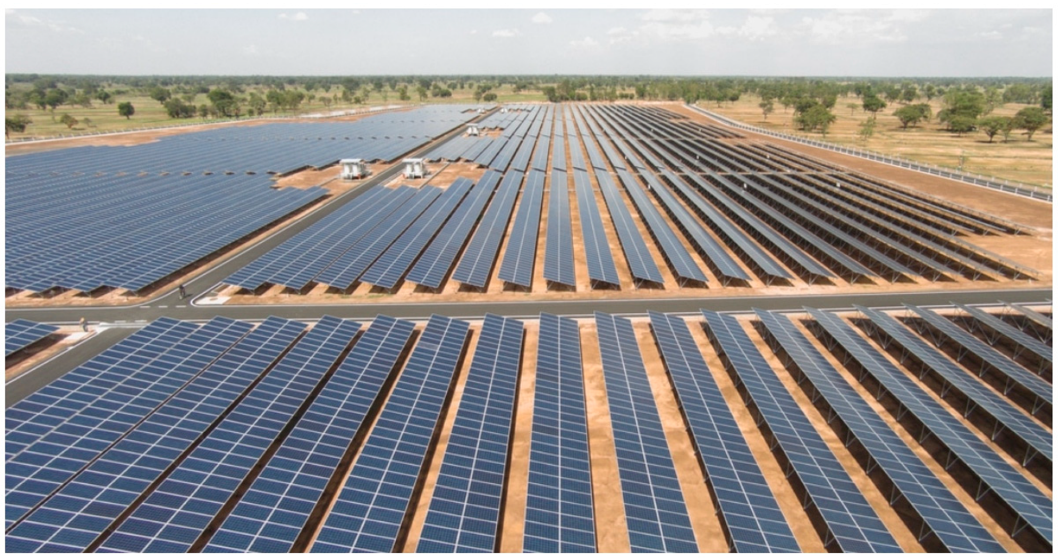
The project’s construction started in January 2020 under a joint venture agreement led primarily by Green Yellow, which held a 95% stake before transferring its entire ownership to AXIAN Energy. Africa Energy Corporation retained the remaining 5% share. The development followed the issuance of a memorandum of understanding (MoU) and a notice to proceed (NTP) by the Ministry of Energy of Burkina Faso, acting through the national electricity utility, SONABEL (Société Nationale d’Électricité du Burkina). Implemented under a public–private partnership (PPP) framework, the project was governed by a long-term power purchase agreement (PPA), ensuring a guaranteed off-take of the generated electricity. The facility has an installed capacity of 30.203 MWp and is designed for an operational lifespan of 25 years, starting from its commercial operation date (COD) in November 2022. Electricity generated by the plant is injected into the national grid via a 33 kV transmission line spanning approximately 21 km, enabling a stable and decentralised energy supply to the surrounding regions and beyond. The photovoltaic array consists of 67,872 high-efficiency monocrystalline silicon modules; each rated at 445 Wp. These modules are mounted on 2424 fixed-tilt support structures and electrically interconnected in strings of 24 panels. Figure 2 shows an overview of Nagréongo’s solar PV plant.
Each string serves as a DC input to one of the 101 SUNGROW transformerless (Sungrow Power Supply Co., Ltd., Hefei, China) inverters, each with a rated output capacity of 250 kVA, designed specifically for high-yield grid-tied solar applications. The inverter outputs are then aggregated and stepped up to a medium voltage using six containerised step-up transformer units, each rated at 4250 kVA, yielding a total transformation capacity of 25.25 MVA. The electrical architecture includes a DC-AC conversion and a medium-voltage interconnection. The plant also includes state-of-the-art monitoring, control, and protection systems that ensure compliance with grid codes, the maximum performance ratio, and an enhanced operational reliability. In addition, the project complied with international standards for environmental and social safeguards, aligning with Burkina Faso’s national electrification strategy and renewable energy goals.

2.2. Data Preparation

The performance assessment of the solar power plant was entrusted to an external consultant as part of the Junior Investigator Research Award (JIRA) project, funded by the Carnegie Corporation of New York through the PASET (Partnership for Skills in Applied Sciences, Engineering and Technology) initiative. This evaluation aimed to ensure technical rigour and transparency in the analysis of the operational efficiency of the plant, while also fostering the development of an early-career research capacity in the field of renewable energy in Sub-Saharan Africa. The independent nature of the assessment helps provide objective information on key performance indicators and loss mechanisms, following international best practices.

2.2.1. Data Collection

In the context of solar energy, an effective performance evaluation is paramount to maximising the efficiency and reliability of photovoltaic (PV) power plants. The ability to accurately collect and analyse data is essential for understanding how these systems operate under varying conditions and for identifying areas for improvement. This part outlines the data-collection framework employed in this study, emphasising the importance of systematic monitoring in assessing the performance of solar plants. The data-collection process encompassed a wide range of parameters, including the energy output, solar irradiance, temperature fluctuations, and operational metrics. By integrating real-time monitoring technologies with manual data-logging methods, this approach aimed to establish a comprehensive dataset that reflected the plant’s operational dynamics over time. In addition, attention was paid to environmental factors that influence the performance, such as weather conditions and site-specific characteristics. All the data were taken from the power plant (on SCADA, meters, and relays) of Nagréongo in Excel format.

2.2.2. Data Cleaning

Following data acquisition, a data-cleaning process was conducted based on the criteria outlined in Table 1, which were extracted from the international standard IEC TS 61724-3 [23]. This process involved the removal of missing values, measurements outside the range, and data affected by abrupt weather changes. Upon the completion of the cleaning process, the weather data—particularly the irradiance values—were verified to ensure consistency with the PVsyst simulation results. According to the PVsyst simulation, the transposition factor between the global horizontal irradiance (GHI) and the incremental irradiance was 1.3. This transposition factor was subsequently calculated and compared across all the available pyranometer datasets.

2.2.3. Losses

To assess the performance, common losses relevant to the study were identified and categorised. These are defined as follows:
O&M losses: These losses are due to equipment failures.
Soil losses: These losses are associated with the dust on the solar modules.
Grid losses: These losses are due to a grid outage.
Qf (U) losses: These losses are due to voltage regulation requests from the grid operator.
Clipping losses: These losses occur when the grid is overloaded, and the inverter power has been clipped for grid protection.
Deemed energy: This is the total of all the energy that has not been produced due to grid unavailability. It covers grid losses, clipping losses, Q = f(U) regulation losses. O&M losses, grid losses, and clipping losses are estimated using the relative comparison (RC) method when at least one inverter does not show any anomalies, or by using the PR reference method when the entire plant is affected by an anomaly. The RC method calculates the unavailability of equipment by comparing its instantaneous production to that of equipment of the same level, under similar conditions. The PR reference method calculates unavailability by taking the performance ratio (PR) of the last point without an anomaly as a reference. The PR formula is shown below:
P R = k P o u t , k × τ k P 0 / k G i , k × τ k G i , r e f
with the following:
  • P o u t , k : AC output of the power plant over time k;
  • G i , k : Average irradiance received during the period;
  • G i , r e f : Reference irradiance, which is 1000 W/m2;
  • P 0 : DC power of the power plant;
  • τ k : Plant availability during period k.
Deemed energy [kWh] = (PRref − PRreal) × actual radiation [kWh/m2] × installed power [kW], where PRref is the average PR of the last 30 min before the occurrence of an anomaly and PR real is the instantaneous PR. The deemed energy due to regulation Q = f(U) is calculated according to the following formulas, with an irradiance threshold >10W/m2:
  • Power: EMD Q = f(U) [W] = Umoy [V] × Imoy [A] × √3 × (cosphi ref − real cosphi)
  • Energy: EMD Q = f(U) [kWh] = EMD Qf(U) [W] × 10/(60 × 1000)
with a cosphi reference of 0.999 as the contract value of cosphi.
A visual inspection was also part of the performance assessment; in fact, it was essential to check if any sensors or equipment was damaged so that the collected data, if needed, could be correlated/explained. A visual inspection was carried out on the solar arrays (panels, mounting structures), but also on the electrical side (DC and AC cabling) and monitoring equipment.

2.3. Forecasting Solar PV Power

The power prediction study of the Nagréongo solar PV plant was conducted as a follow-up to the performance assessment, to explore the feasibility of implementing a forecasting system that surpasses traditional statistical methods in terms of accuracy and responsiveness. This advanced modelling approach aims to support the grid operator in the optimal management of the electricity demand and to enable the plant operator to forecast the energy output with a greater precision. In this context, state-of-the-art deep learning techniques—namely long short-term memory (LSTM), gated recurrent units (GRUs), recurrent neural networks (RNNs), and hybrid LSTM-GRU models—were explored. These models are known for their ability to learn temporal patterns and dependencies from historical data, making them particularly well suited for solar energy forecasting under variable climatic conditions. Their application in this study is expected to contribute to improving grid stability, improving the integration of intermittent renewable sources, and supporting data-driven decision making in power system operations.

2.3.1. Recurrent Neural Networks (RNNs)

Recurrent neural networks (RNNs) are a class of artificial neural networks that are particularly well suited for processing sequential data, such as time series, natural language, or sensor readings. Unlike traditional feedforward neural networks, which assume that all inputs are independent of each other, RNNs maintain a form of memory that allows information to persist across time steps. This architecture makes them particularly effective for tasks that involve temporal dynamics and contextual dependencies [24]. In an RNN, the output from a previous time step is fed back into the network along with the current input. This loop structure enables the network to exhibit temporal behaviour and learn patterns over sequences. The key idea is that, at each time step t, the network takes an input xt, processes it along with the hidden state ht−1 from the previous time step, and produces a new hidden state ht. Mathematically, this can be expressed by Equation (2):
ht = f (Wh·ht−1 + Wx·xt + b)
where f is typically a non-linear activation function such as tanh or ReLU.
Despite their potential, standard RNNs suffer from certain limitations when dealing with long sequences, primarily due to the vanishing or exploding gradient problem during training. This challenge prevents the network from learning long-term dependencies effectively [25]. To address this, more advanced variants such as long short-term memory (LSTM) and gated recurrent units (GRUs) were introduced [26,27]. Nevertheless, basic RNNs remain a fundamental building block in deep learning and are still widely used in lightweight applications, particularly where memory efficiency and model simplicity are preferred. Research has shown that RNNs are applied in forecasting applications in domains such as renewable energy [28]. In the context of solar energy, for example, RNNs have been used to predict the short-term solar irradiance and photovoltaic output with moderate success, especially when combined with data preprocessing and ensemble strategies [29]. Figure 3 represents the architecture of a standard RNN.
In a standard RNN, each input at a time influences the hidden state and output of the same step, with hidden states passing information forward through time.
Despite their simplicity, RNNs offer a foundational understanding of how deep learning can be applied to sequence modelling. Their core mechanism of temporal recurrence has inspired numerous innovations in neural architecture, particularly those related to attention mechanisms and transformers [26], which often build on or replace traditional RNN structures for more complex tasks.

2.3.2. Long Short-Term Memory (LSTM) Model

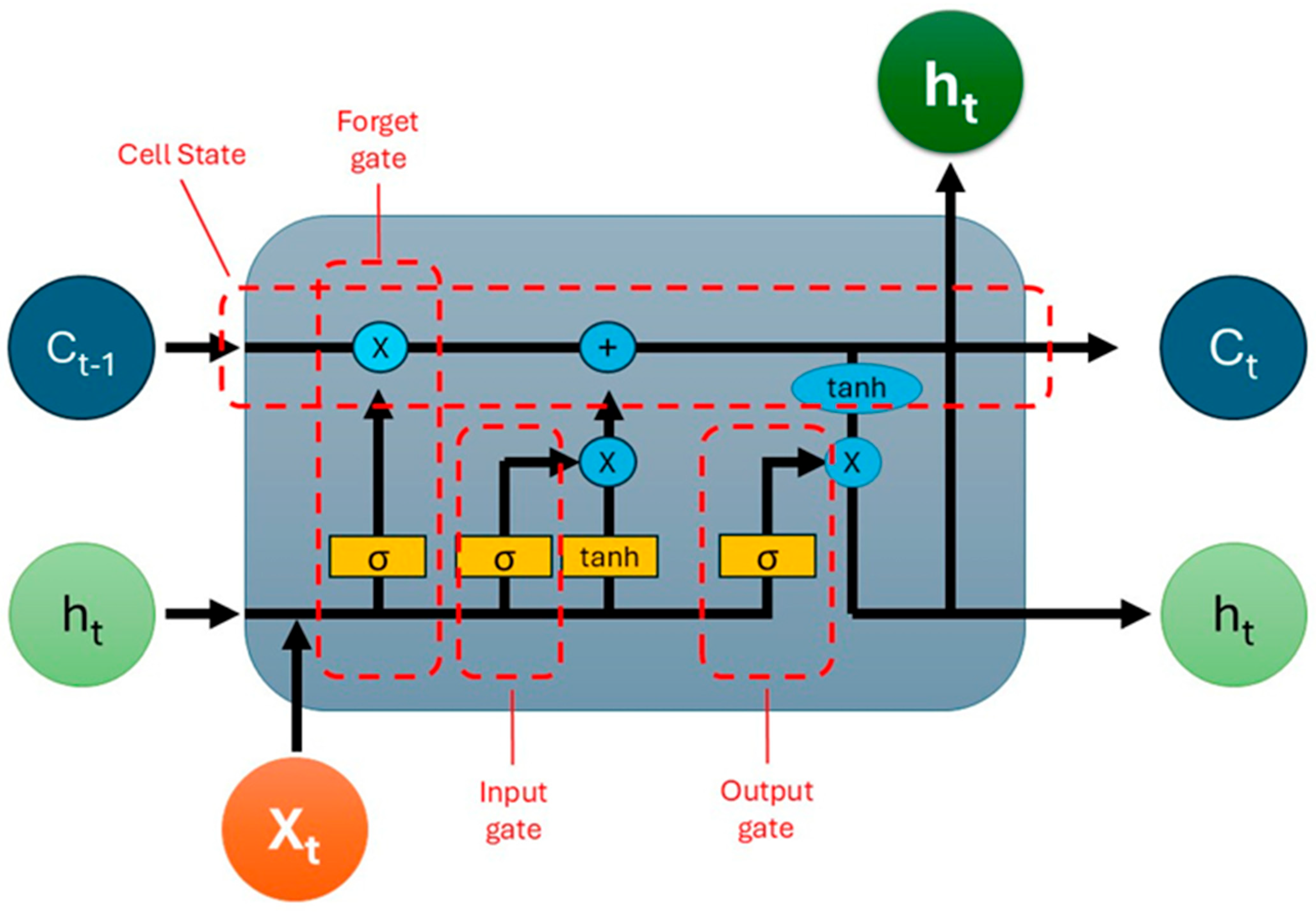
Long short-term memory (LSTM) networks are a specific type of recurrent neural network (RNN) designed to model sequential data and capture long-term dependencies, effectively addressing the limitations of traditional RNNs such as vanishing and exploding gradients [31]. Unlike standard RNNs, which tend to forget earlier parts of sequences as they grow longer, LSTMs incorporate memory cells and gating mechanisms that allow them to retain and selectively forget information across time steps. Each LSTM unit comprises three gates: the input gate, the forget gate, and the output gate. These gates control the flow of information into, within, and out of the memory cell. The forget gate determines what portion of the past cell state should be discarded. The input gate regulates the amount of new information to be added to the cell state, while the output gate decides what part of the current cell state should be output to the next step [32]. This architecture enables the LSTM to learn complex temporal patterns and long-term dependencies in time-series data, making it particularly effective for forecasting and classification tasks in domains such as renewable energy [33], financial markets [34], and speech recognition [35]. Recent studies have demonstrated the superiority of LSTM models over classical statistical approaches in forecasting solar photovoltaic (PV) power outputs, due to their ability to capture non-linear dependencies and variability caused by atmospheric conditions [29]. For example, in renewable energy forecasting, LSTM networks have been used to predict short-term solar power generation with a greater accuracy than ARIMA and persistence models [36]. The general structure of an LSTM cell is illustrated in Figure 4 below:
LSTM networks are often used with dropout regularisation and normalisation techniques to avoid overfitting, particularly when training on small datasets [38]. In practice, the implementation of LSTM models is facilitated by machine learning libraries such as TensorFlow and PyTorch through google colaboratory, which allow for the customisation of the number of layers, hidden units, activation functions, and learning rates.

2.3.3. Gated Recurrent Unit (GRU) Networks

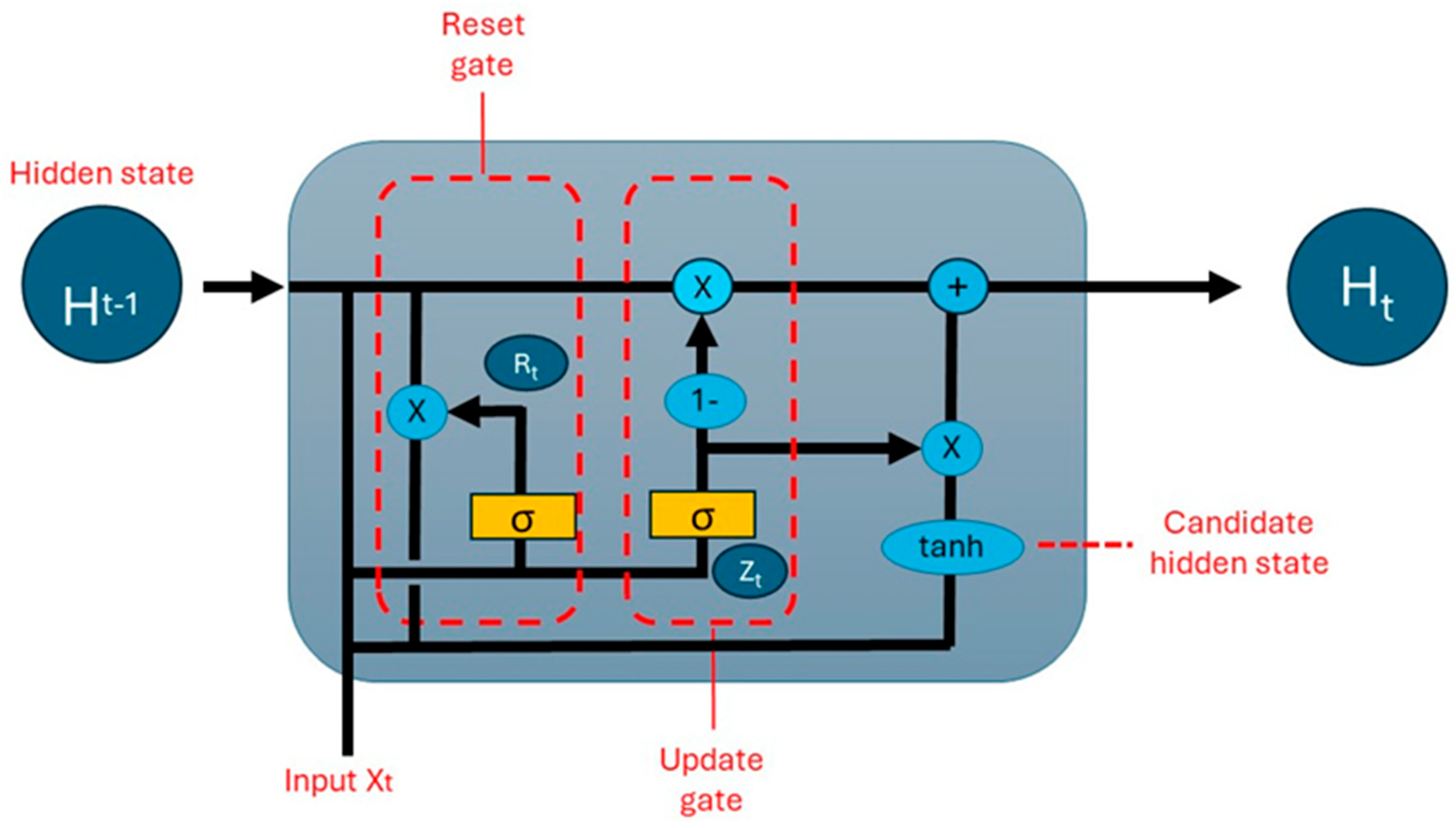
Gated Recurrent Units (GRUs) are a variant of recurrent neural networks (RNNs) designed to capture dependencies in sequential data while addressing the limitations of standard RNNs. Introduced by [39], GRUs simplify the architecture of long short-term memory (LSTM) networks by combining the forget and input gates into a single update gate and merging the cell and hidden states. This makes GRUs computationally more efficient while maintaining a comparable performance in many sequence-modelling tasks. The simplicity of this architecture allows GRUs to converge faster and require less memory compared to LSTMs [39]. GRUs have demonstrated a strong performance on a wide range of tasks, including renewable energy forecasting, natural language processing, and anomaly detection in time-series data [40]. In solar photovoltaic (PV) output prediction, GRUs have been shown to outperform traditional statistical models and even LSTMs in certain short-term forecasting contexts, particularly when data are limited or model interpretability is required [40]. Figure 5 shows a diagram of a GRU cell.
Due to their streamlined structure, GRUs are especially suitable for real-time applications and embedded systems where computational efficiency is crucial. They have been widely adopted in smart grid forecasting systems, IoT-based monitoring frameworks, and hybrid deep learning models [41]. Moreover, GRUs tend to generalise well in scenarios with small to moderate amounts of training data, making them highly practical in developing regions or emerging sectors.

2.3.4. Evaluation of the Performance of the Forecast Model

A performance evaluation of machine learning models in photovoltaic (PV) power forecasting typically relies on key statistical indicators such as the coefficient of determination (R2), root mean square error (RMSE) and mean absolute error (MAE). These metrics are essential to assess the accuracy and reliability of model predictions. The RMSE quantifies the average magnitude of prediction errors by taking the square root of the mean squared differences between the predicted and actual values. It is sensitive to large errors, making it a useful measure when such deviations are of concern. It is expressed by Equation (3) below [28,42]:
R M S E = 1 n i = 1 n ( y i y ^ i ) 2
 
The MAE, on the other hand, measures the average absolute difference between the predicted and actual values. It treats all errors equally, making it straightforward to interpret and robust against outliers. It is given by Equation (4) [41]:
M A E = 1 n i = 1 n y i y ^ i
To allow for a fair comparison across different datasets or systems with varying scales, normalised versions of the RMSE and MAE are often employed. The normalised RMSE (nRMSE) and normalised MAE (nMAE) are obtained by dividing the RMSE and MAE by either the mean or the range of observed values, and are expressed as a percentage as given by Equations (5) and (6), respectively:
n R M S E = R M S E y × 100 %
n M A E = M A E y × 100 %
where y is the mean of the actual observations. The coefficient of determination (R2) indicates how well the predicted values match the observed data. A value close to 1 implies that the model explains a large proportion of the variance in the data, and therefore provides more reliable predictions [43].
R 2 = 1 i = 1 n ( y i y ^ i ) 2 i = 1 n ( y i y i ) 2
In summary, a good predictive model should aim for a low RMSE and MAE (and correspondingly, a low nRMSE and nMAE) and an R2 value approaching 1, indicating both accuracy and reliability in forecasting the PV power output. Table 2 below highlights the normal ranges of performance metrics for the implementation of deep learning models for PV power forecasting.

2.3.5. Dataset for Prediction

  • Data choice and preprocessing
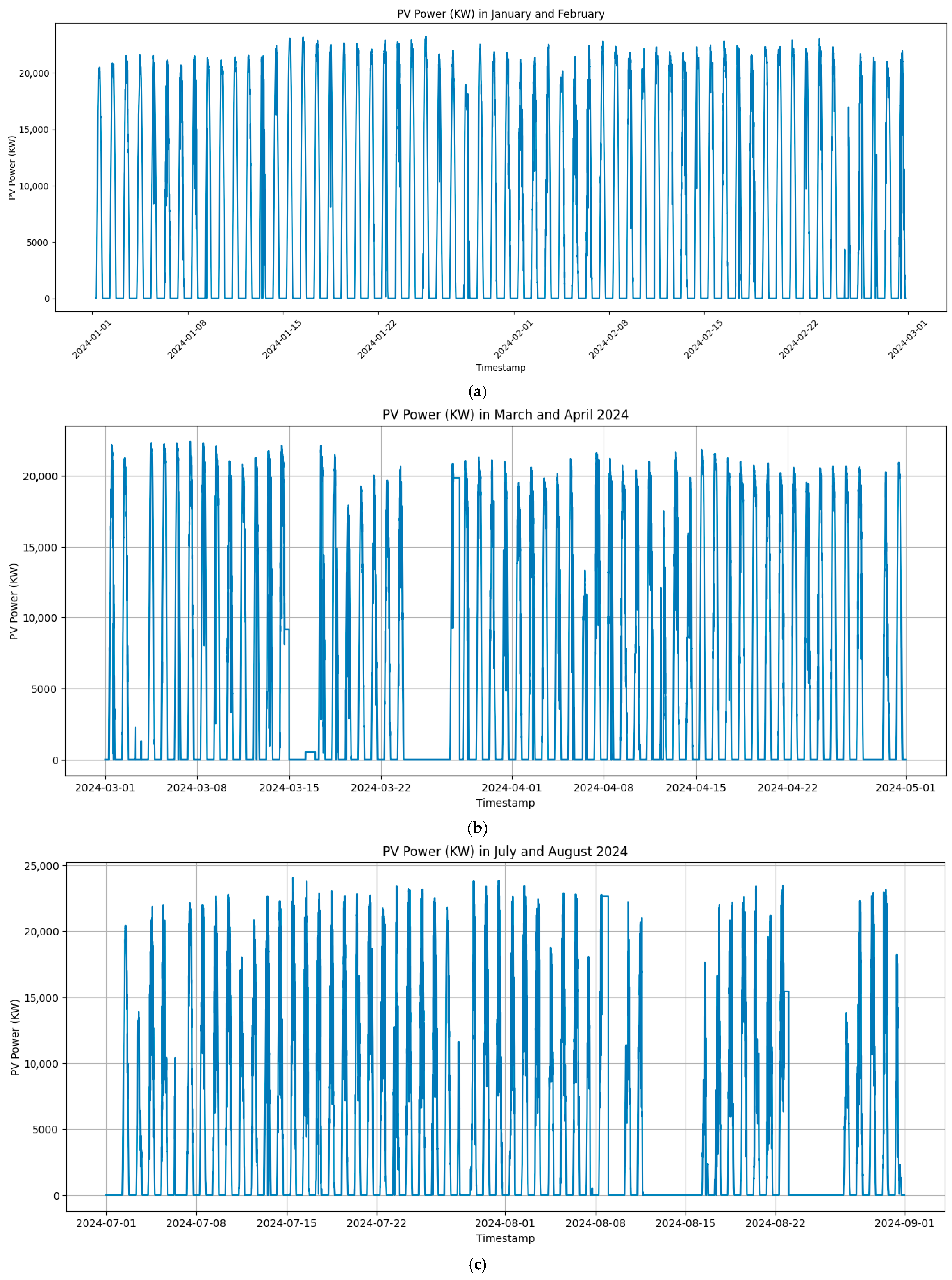
Discussions with the consultant confirmed that the January–February 2024 dataset contained minimal curtailment or operational disruptions, making it highly representative of standard operating conditions. To improve the robustness and capture seasonal variability, additional datasets from March–April and July–August 2024 were used, with all incomplete days removed. These high-frequency (5 min resolution) records provide consistent, noise-reduced inputs for training deep learning models to forecast the PV power output at the Nagréongo plant. Incorporating both dry and rainy season data ensures that the models learn from diverse weather conditions, thereby enhancing their generalisation capacity, improving their short-term prediction accuracy, and reducing their sensitivity to missing or noisy values. Figure 6a–c show the temporal evolution of daily PV generation during January–February, March–April, and July–August in 2024, respectively, illustrating the typical production patterns at the site.
  • Hyperparameters
All the models shared identical training hyperparameters, including epochs, batch sizes, and validation splits, as well as the same callback strategies, such as early stopping and learning rate reduction, ensuring a fair comparison that isolated the effect of architectural choices. The main difference lies in the recurrent layers: An RNN is efficient, but limited for long-term dependencies; LSTM uses gates to retain and forget information, improving the sequence modelling; a GRU is a leaner version of LSTM, and is faster to train with fewer parameters; and the hybrid model combines LSTM and a GRU to leverage both the long-term memory and the training efficiency. Dropout with a rate of 0.2 after each recurrent layer helps mitigate overfitting by randomly deactivating neurons during training, improving generalisation. The dense layers, with 50 units followed by a single-unit output layer, refine the learned features and produce the final regression prediction for PV power. The Adam optimiser provides adaptive learning rate optimisation, balancing the efficiency and convergence stability, while the mean squared error loss function penalises large errors appropriately for regression tasks. Finally, the callbacks—early stopping to halt training when the validation loss plateaus and reduce LR on plateau to lower the learning rate when progress stagnates—further improve convergence and prevent overfitting. Overall, while the training pipeline is consistent across models, the choice of the recurrent cell remains the key factor influencing the temporal dependency capture, training efficiency, and predictive accuracy. The details of all the hyperparameters used to run the deep learning models are presented in Table 3.

2.3.6. Process for Prediction

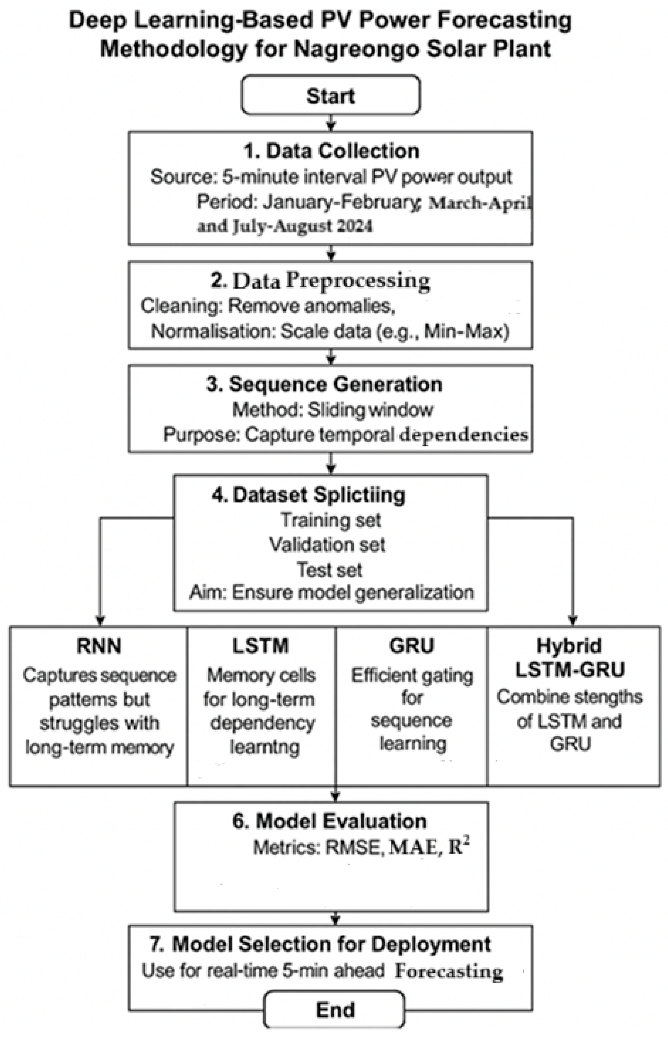
The process began with data cleaning and normalisation to prepare the time series for modelling. Input–output sequences were then generated using a sliding window approach to capture temporal dependencies. The dataset was divided into training session (80% of data) and validation and testing (20% of data) subsets to ensure model robustness. Each model was trained to learn short-term patterns in PV generation using past PV power values to predict the future output at 5 min intervals. RNNs capture sequential patterns but often struggle with long-term dependencies. LSTM and GRUs overcome this through memory cells and gating mechanisms, improving the accuracy in dynamic weather conditions. Hybrid LSTM-GRU models combine both strengths and offer an improved convergence and performance [43,47]. After training, the models were evaluated using the RMSE, MAE, and R2. Lower error values and a higher R2 indicated a better performance. The most accurate model was then used for operational forecasting, supporting grid stability and energy management. Figure 7 represents the flowchart explaining the steps used for this study.

3. Results and Discussions

3.1. Performance Analysis

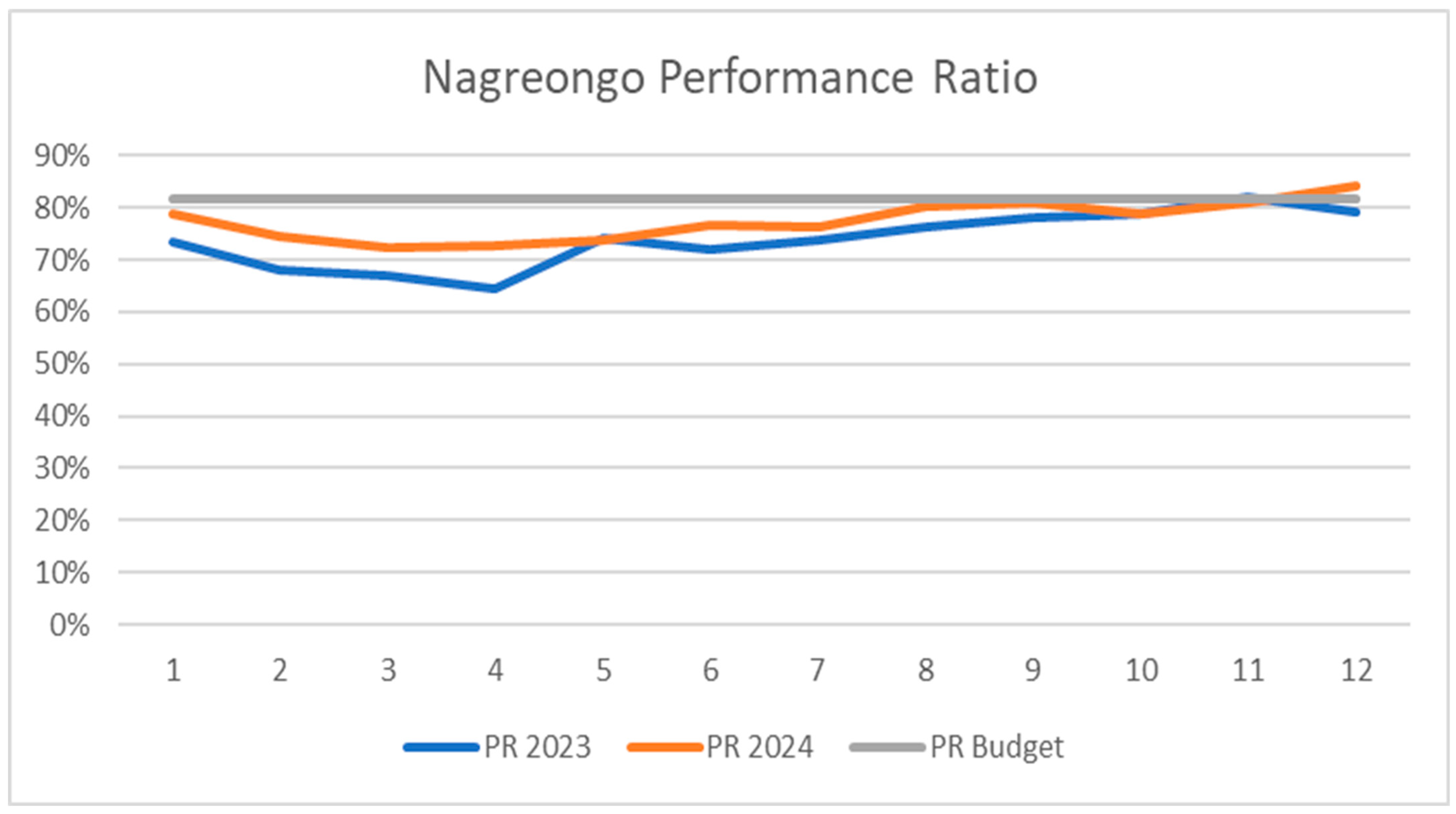
The performance assessment revealed an annual performance ratio (PR) of 73.73% in 2023, which improved to 77.43% in 2024. This increase indicates an enhanced system efficiency and operational effectiveness over time. The monthly evolution of the PR, as illustrated in Figure 8, provides further insight into the seasonal variations, system reliability, and potential performance optimisation achieved throughout the year.
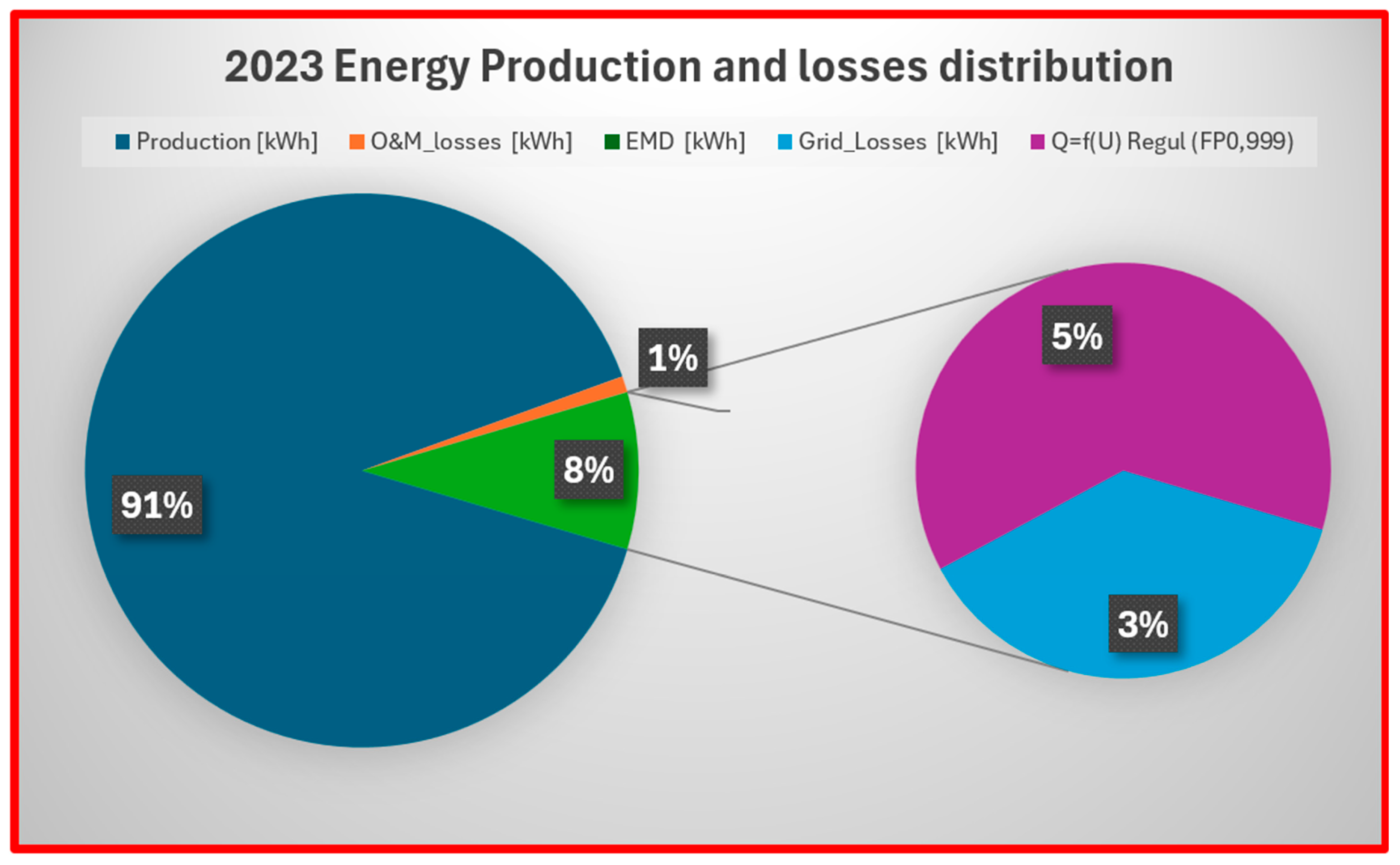
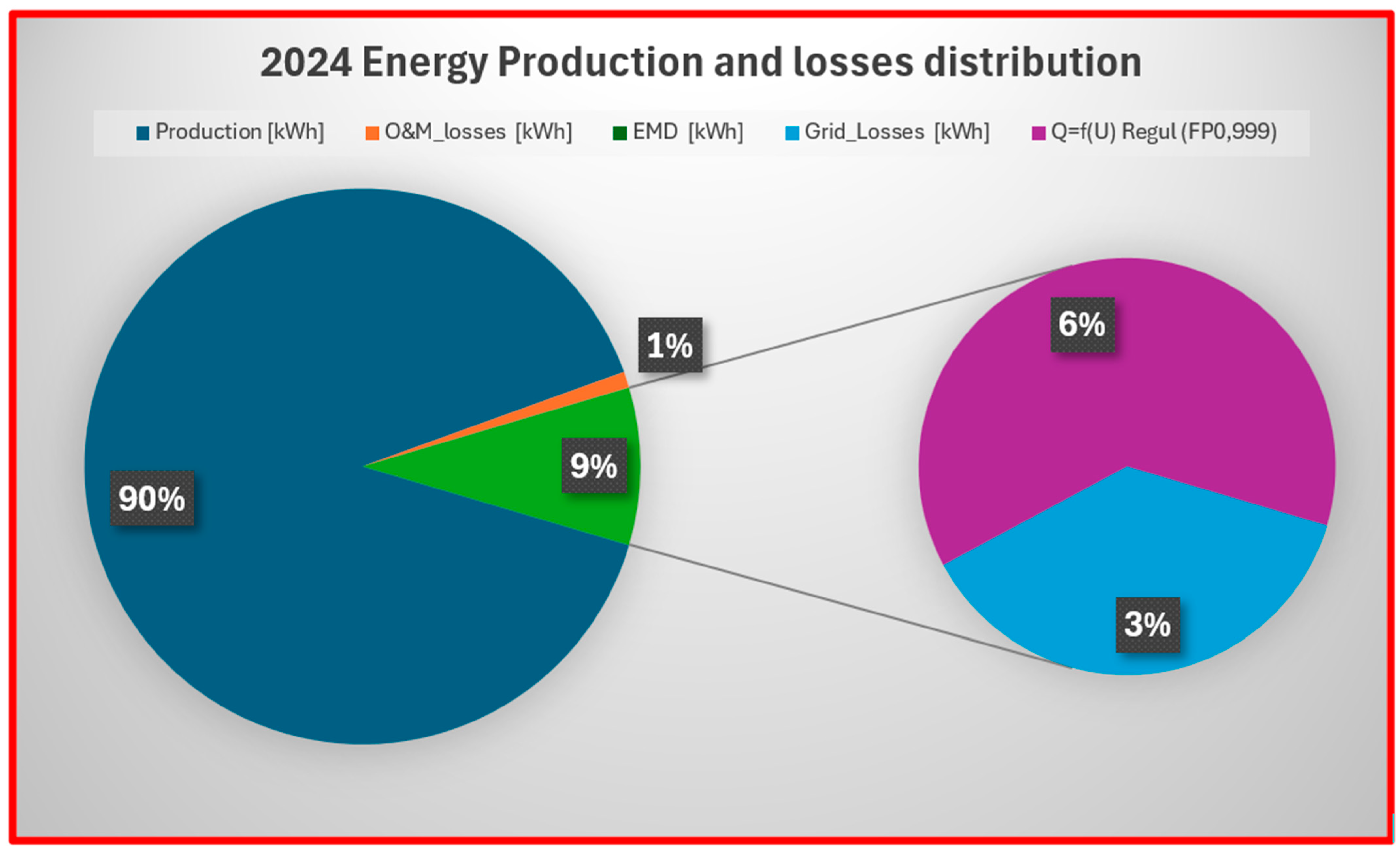
The various losses in the system were quantified and categorised for 2023 and 2024. In both years, voltage regulation losses emerged as the dominant category, accounting for nearly half of the total losses, followed by grid-related losses. The respective contributions of each loss component are illustrated in the pie charts below (Figure 9 and Figure 10), providing a comparative overview of the distribution of losses over the two years.
To better understand the trend, figures, and events that may have impacted the performance, a discussion was held with the stakeholders (plant operators and managers). After a discussion with the operators and the plant manager, three major events were detected that affected plant performance:
Grid congestion at the Ziniaré substation: An evacuation line at 90 kV was planned to be built between Ziniaré and Kossodo. Ziniaré is the nearest substation where the production of the Nagréongo power plant is carried out. Therefore, the plant cannot produce the maximum power due to the voltage and current restrictions of the grid. The temporary solution that was found was to implement voltage and current regulation, which has an impact on the performance of the plant. In September 2024, an agreement was reached with the grid operator, and the voltage and current regulation were disabled.
The impact of soiling in 2023: From the commissioning of the plan up to May 2023, there was no cleaning equipment for the solar plant. During this period, the soil loss was high, as the plant was not cleaned. After purchasing a cleaning tractor in June 2023, the performance became high during the dry season because the plant was cleaned. As a result, the soil erosion losses were low during 2024.
Power outage: Burkina Faso went through a severe power outage from March 2024 to June 2024. Therefore, the plant was subjected to many power outages. The grid operator put in place a power-shedding plan to stabilise the grid and reduce outages.
From the discussion with the operators, it was outlined that there was an inverter spare parts shortage between November 2023 and February 2024.
When analysing the performance ratio of 2023 and 2024, we can see that the 2024 performance was better than the 2023 performance. The PR budget was reached in November 2024 and even exceeded the budget in December 2024, as can be seen in Figure 11 below. These improvements were due to the control of voltage regulation and the cleaning of the tractor’s operation.
The conducted evaluation highlighted some challenges in the operation and maintenance activities that need to be addressed. The first major challenge is related to the requirements of the national grid operator to maintain grid stability. The second challenge is related to the maintenance strategy, given the lack of some KPIs that could be used for decision making.
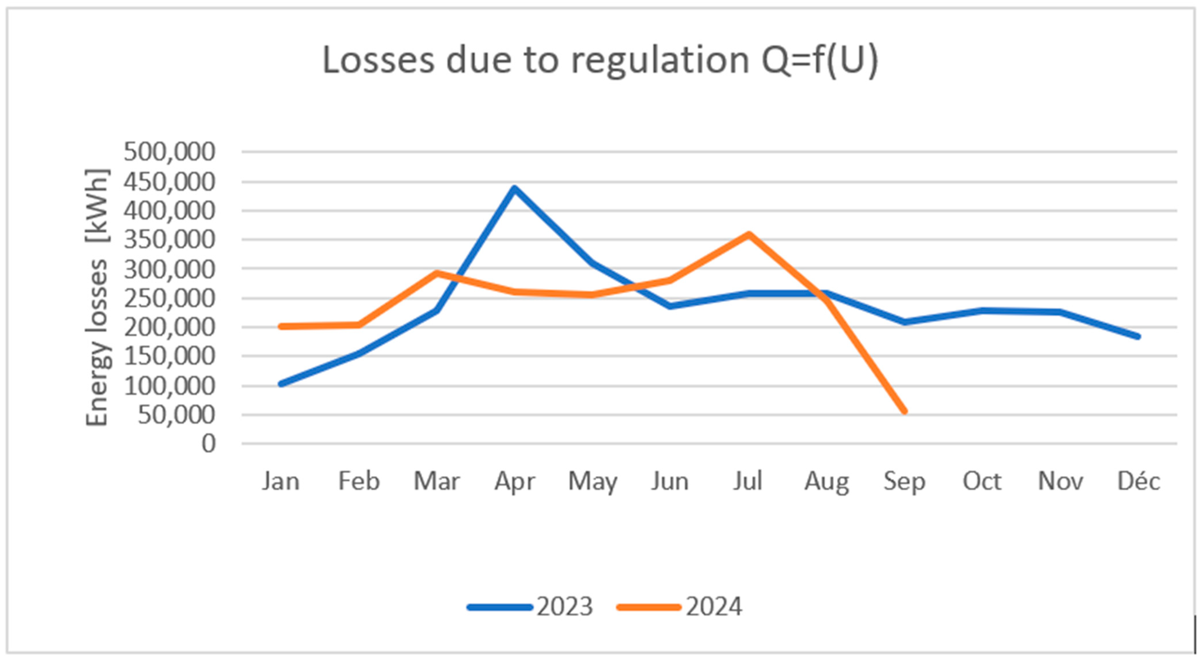
The solar plant, during its first two years, was required by the grid operator to implement the Q = f(U) regulation function to maintain grid stability. This implementation reduced the amount of active power that could be fed to the grid, thus reducing the overall output of the plant, which, in turn, impacted the performance. This represents the largest contribution to the total losses of the plant, at 56% in 2023 and 49% in 2024. As can be noticed in Figure 12 below, in September 2024, the regulation was turned off.

3.2. PV Power Forecasting

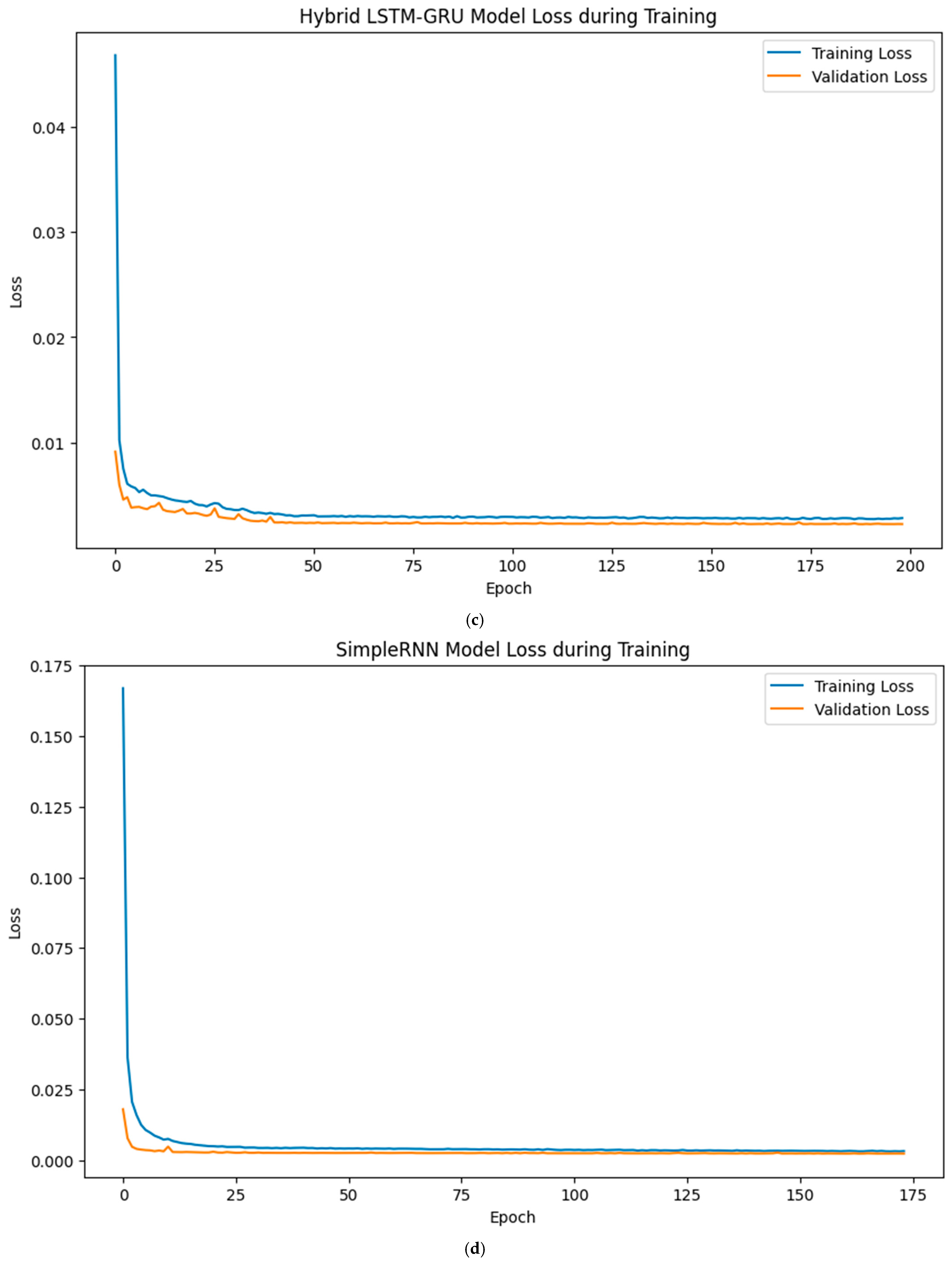
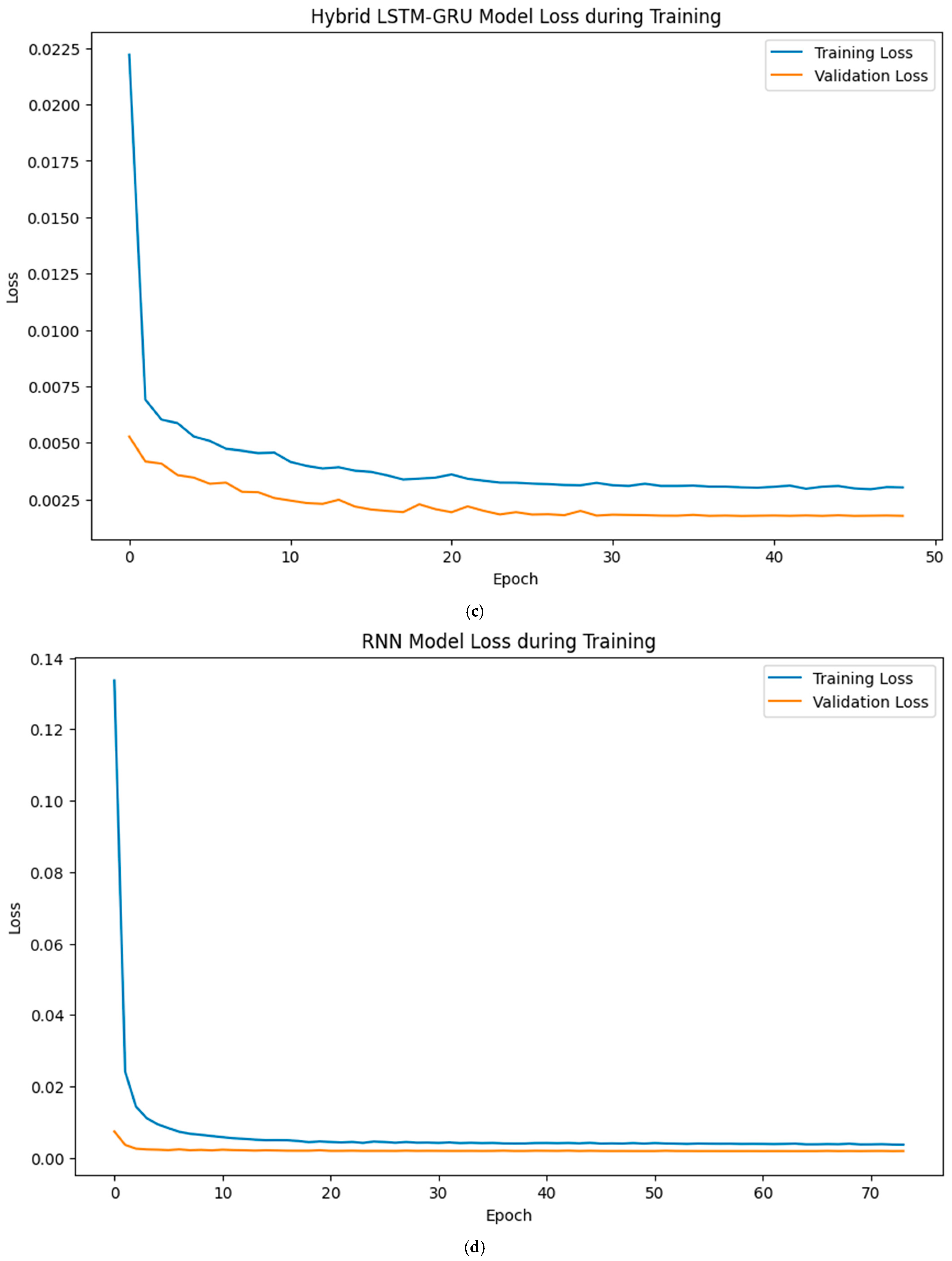
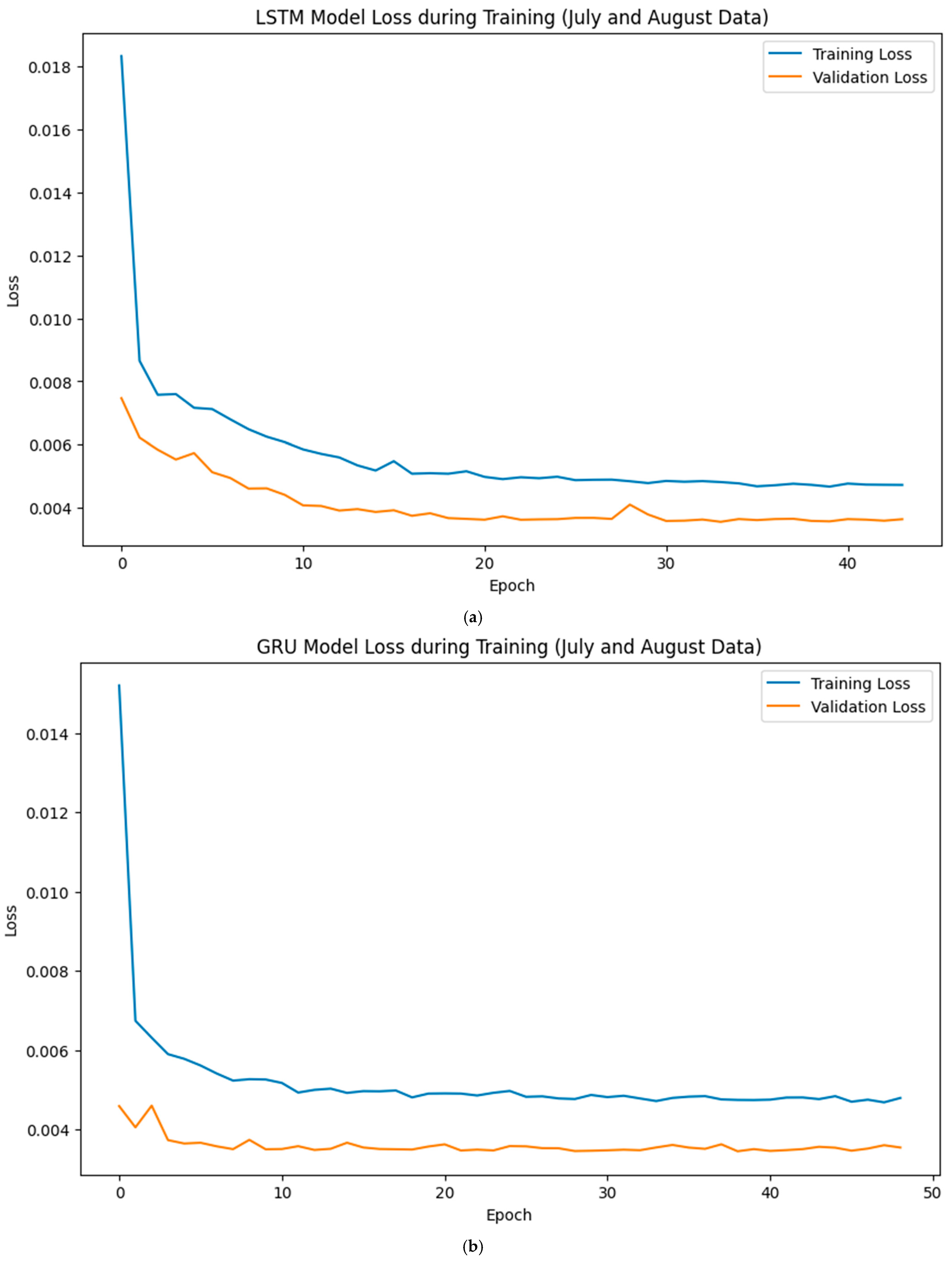
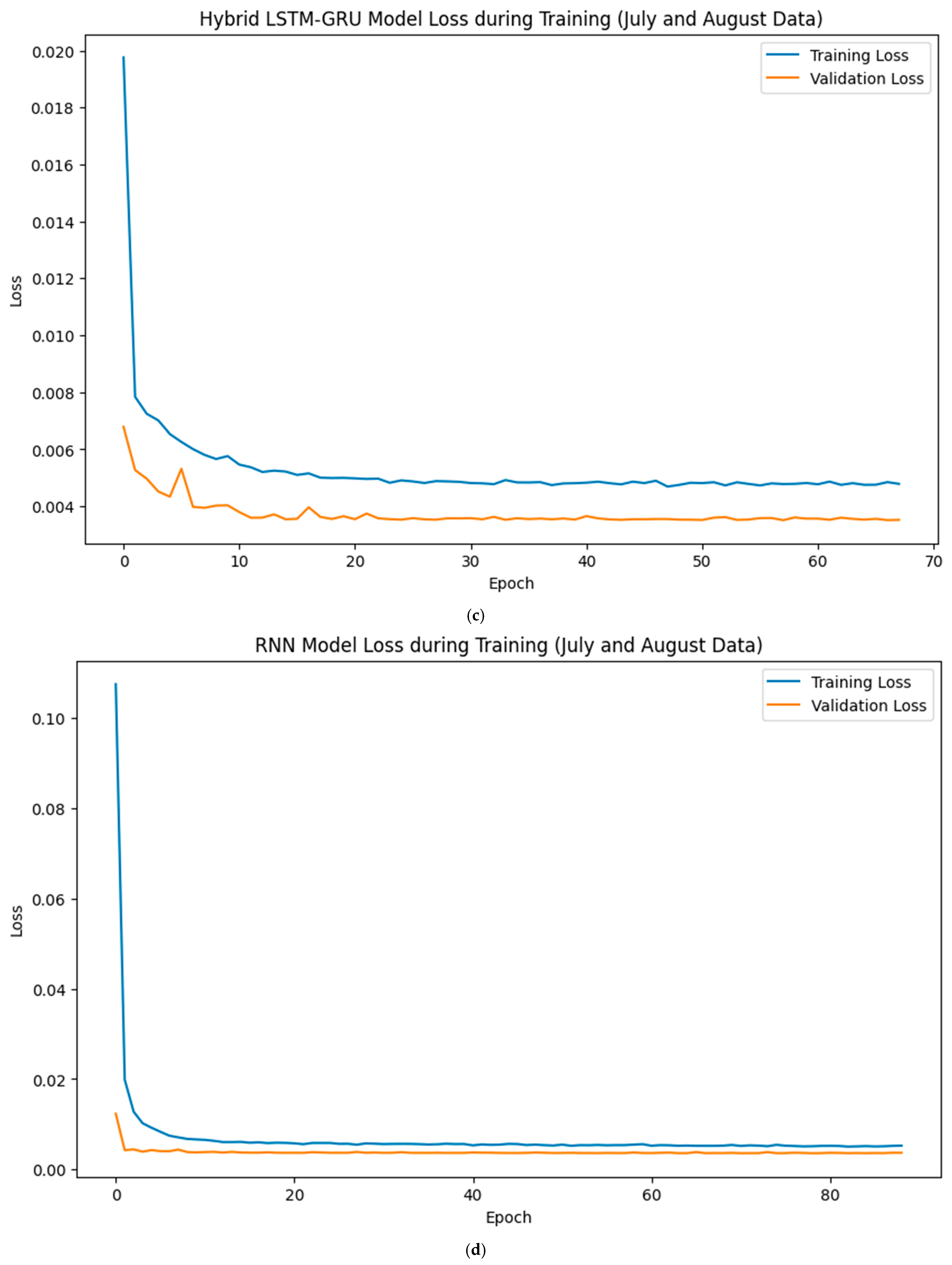
All the loss curves in Figure 13a–d, Figure 14a–d, and Figure 15a–d (January and February, March and April, and July and August, respectively), which represent the evolution of training and validation loss for the LSTM, GRU, LSTM-GRU, and RNN models, respectively, showed a clear downward trend, indicating effective convergence and proper model generalisation. The training and validation losses remained closely aligned throughout the epoch, with no significant divergence or overfitting, suggesting that appropriate training regimes and regularisation strategies were employed. The forecasting results obtained for the 30 MW Nagréongo solar photovoltaic (PV) plant in Burkina Faso demonstrate the effectiveness of recurrent neural network (RNN)-based architectures in modelling PV power generation under varying climatic conditions in 2024. The analysis reveals that the predictive performance of the models was strongly influenced by the seasonal weather regimes that characterise the Sahelian climate.
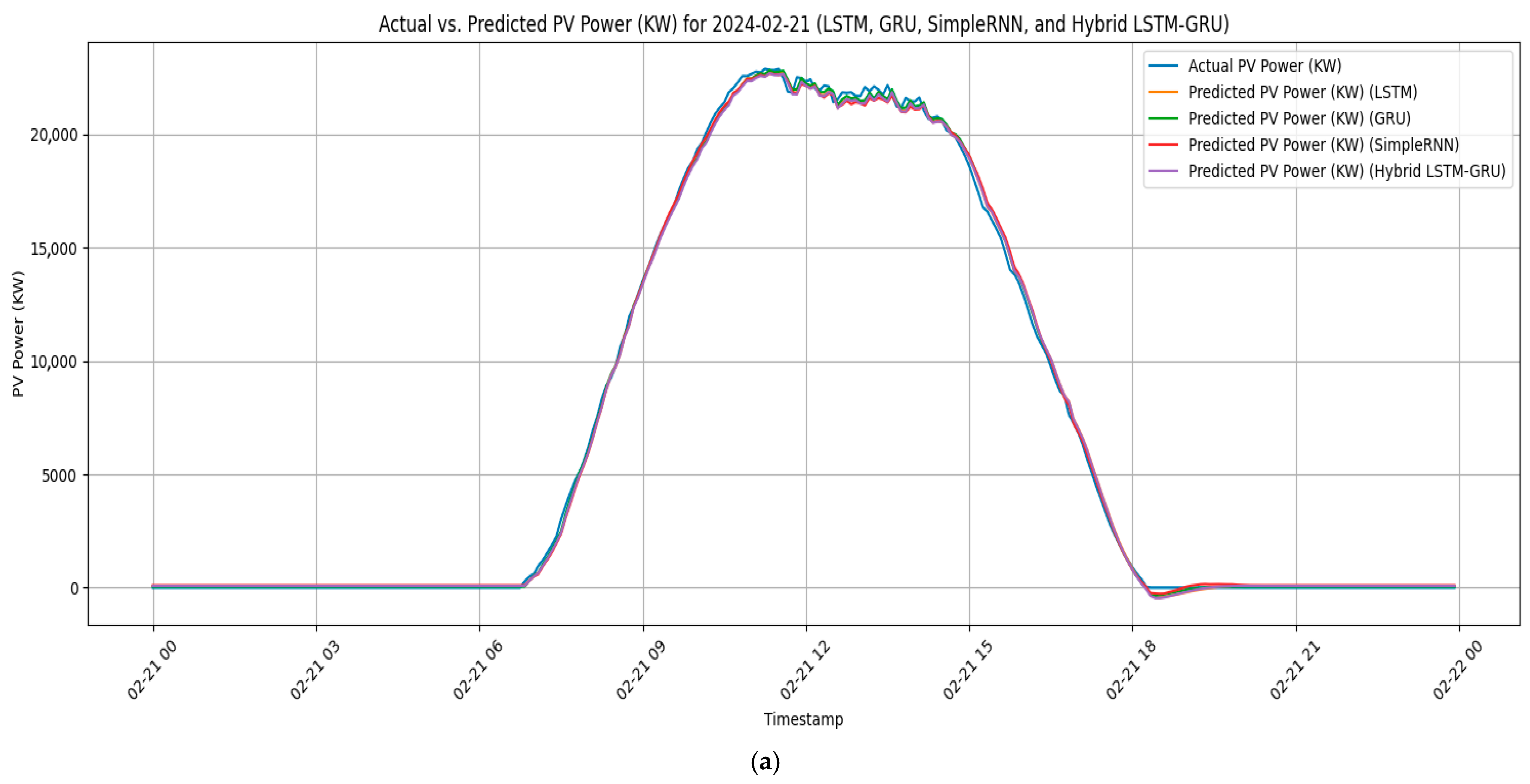
During January–February (dry season), all the models exhibited a strong forecasting accuracy, with the gated recurrent unit (GRU) model achieving the best performance (test RMSE = 1290 kW, nRMSE = 4.30%, R2 = 0.978). Errors remained below 5% of the plant’s nominal capacity, suggesting that the relatively stable irradiance patterns during this period were well captured by memory-based architectures. These findings are consistent with previous studies, which have reported an improved performance of GRU models in environments with limited short-term variability [48].
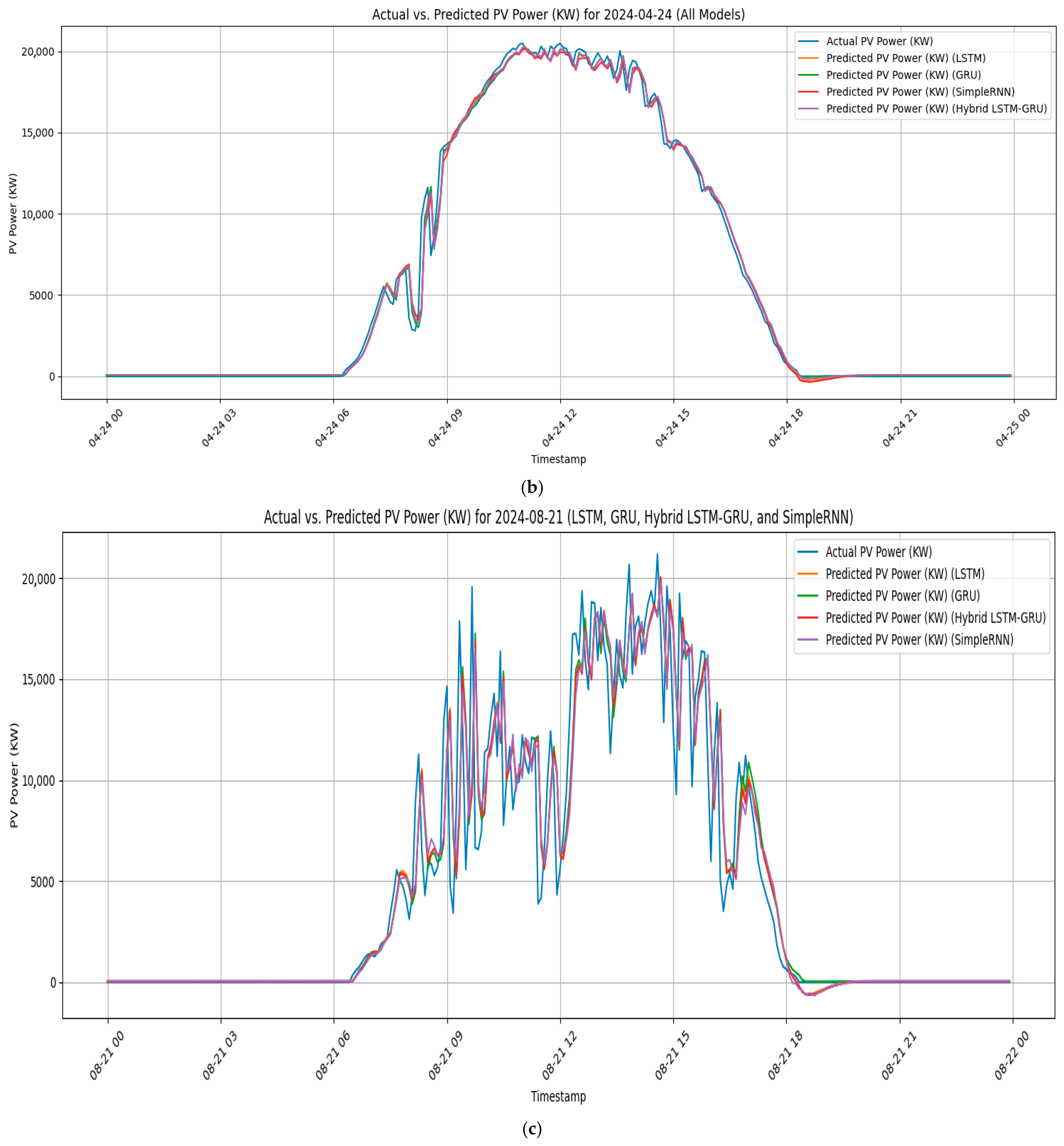
In March–April (hot season), the accuracy further improved across all architectures, with the normalised RMSE values approaching 2% of the plant capacity. The long short-term memory (LSTM) model achieved the lowest errors (test RMSE = 618 kW, nRMSE = 2.06%, MAE = 260 kW) and the highest coefficient of determination (R2 = 0.994). This highlights the capacity of LSTM cells to capture complex temporal dependencies and diurnal variability associated with the high irradiance and increasing atmospheric instability typical of this season. The superior performance of LSTM during transitional months indicates its suitability for short-term PV power forecasting when rapid fluctuations occur [49].
In contrast, July–August (rainy season) posed greater challenges, with the forecasting errors increasing to over 5% of the nominal capacity for all the models. The hybrid LSTM-GRU model provided the most balanced performance, achieving the lowest test MAE (723 kW; nMAE = 2.41%), while the GRU slightly outperformed in terms of the RMSE (1641 kW; nRMSE = 5.47%). The reduced accuracy reflects the significant variability in solar irradiance caused by cloud cover and precipitation during the West African monsoon season. Nevertheless, the results confirm that hybrid approaches can enhance the robustness under conditions of a high stochasticity, mitigating some of the limitations of individual architectures.
Overall, this study demonstrates that RNN-based models can achieve forecasting errors within 2–5% of the nominal PV capacity across different seasons, a level of accuracy that is generally sufficient to support grid integration, energy dispatch, and operational planning in utility-scale PV plants. The comparative analysis further indicated that model selection should consider seasonal climatic regimes: A GRU is more effective during stable dry periods, LSTM outperforms in transitional months with pronounced diurnal variability, and hybrid LSTM-GRU models are advantageous under rainy season conditions characterised by a high uncertainty. These findings provide valuable insights for the deployment of advanced forecasting tools in Sub-Saharan Africa, where the increasing penetration of solar energy requires accurate and adaptive predictive models to ensure system reliability and energy security. Table 4 summarises the training and testing results of the four deep learning models.
Figure 16a–c illustrate the daily evolution of the actual and predicted PV power output from the Nagréongo solar plant for the months of January–February (dry season), March–April (hot season), and July–August (rainy season) in 2024, respectively, using the deep learning methods LSTM, a GRU, LSTM-GRU, and an RNN. The predicted curves show a strong alignment with the measured values, confirming the effectiveness of these models in capturing the temporal dynamics of PV generation under varying climatic conditions. This close agreement demonstrates that the models are not only capable of reproducing diurnal production profiles, but also of adapting to seasonal variability typical of the Sahelian environment. The results further highlight the capacity of memory-based architectures to generalise across distinct weather regimes, with minimal deviation between the predicted and actual power curves. Such a performance underscores the reliability of deep learning approaches for operational forecasting, providing valuable support for grid stability, energy dispatch, and planning in regions with rapidly expanding solar penetration.

4. Conclusions

This study demonstrated the critical importance of accurate power prediction models in improving the operational efficiency and management of large-scale photovoltaic systems, using the Nagréongo solar PV power plant in Burkina Faso as a case study. A seasonal analysis revealed that GRU models perform best during the dry season, capturing stable irradiance patterns effectively, while LSTM excels during transitional months, handling rapid diurnal variations with a higher precision. During the rainy season, hybrid LSTM-GRU models offer the most balanced performance, mitigating the impact of a high variability in solar irradiance due to cloud cover and precipitation. The performance evaluation conducted by an external consultant confirmed the strong technical efficiency of the plant, with a significant improvement in its performance ratio from 73.73% in 2023 to 77.43% in 2024. This positive trend underscores the value of continuous monitoring and intelligent management systems.
These findings highlight the importance of selecting forecasting models that are adaptive to local climatic regimes, particularly in West African contexts, where the seasonal variability strongly influences PV generation. The accuracy achieved by deep learning model approaches in this study is sufficient to support operational planning, grid integration, and energy dispatch decisions, thereby enhancing the reliability and economic efficiency of utility-scale PV plants.
Looking ahead, future research could explore the integration of real-time meteorological data, satellite imagery, and hybrid models that combine machine learning with physics-based forecasting. Moreover, extending the forecasting horizon to medium- and long-term scales, while ensuring interpretability and model robustness, would be beneficial for strategic energy planning. Lastly, replicating this approach for other solar installations in the Sahel region could support the larger goal of sustainable energy access and climate resilience in Sub-Saharan Africa.

Author Contributions

Conceptualisation, S.F.P., A.G., and S.M.K.; methodology, S.F.P., A.G., and S.M.K.; software, S.F.P. and A.G.; validation, D.B., A.L.O., Y.M.S., and M.S.; formal analysis, Y.M.S., S.F.P., S.M.K., and D.B.; investigation, S.F.P. and A.G.; resources, Y.M.S. and M.S.; data curation, S.F.P. and A.G.; writing—original draft preparation, S.F.P.; writing—review and editing, A.G., S.M.K., D.B., A.L.O., Y.M.S., and M.S.; visualisation, S.F.P., A.G., and S.M.K.; supervision, Y.M.S. and M.S.; project administration, Y.M.S. and M.S.; funding acquisition, Y.M.S. and S.F.P. All authors have read and agreed to the published version of the manuscript.

Funding

The work was carried out with the financial support of the Carnegie Corporation in New York to the PASET Regional Scholarship and Innovation Fund (RSIF) DOCTAS project, through the International Centre of Insect Physiology and Ecology (ICIPE), grant Ref. G-22-59858. The views expressed herein do not necessarily reflect the official opinion of the donors.

Data Availability Statement

The data presented in this study are available on request from the corresponding author due to confidentiality from the plant management.

Acknowledgments

The authors would like to thank the company NEA BURKINA, a subsidiary of AXIAN ENERGY, for its contribution.

Conflicts of Interest

The authors declare no conflicts of interest.

Abbreviations

The following abbreviations are used in this manuscript:
PVPhotovoltaic
LSTMLong Short-Term Memory
GRUGated Recurrent Network
RNNRecurrent Neuron Network

References

  1. International Energy Agency. World Energy Outlook 2023. Available online: www.iea.org/terms (accessed on 5 July 2025).
  2. Bariloche, F. Module Overview Policy and Targets Investment and Finance Challenges and Opportunities. SCIENCE AND ACADEMIA AEE-Institute for Sustainable Technologies (AEE-INTEC) Council on Energy, Environment and Water (CEEW). 2024. Available online: https://www.ren21.net/gsr-2024/modules/global_overview/04_challenges/ (accessed on 5 July 2025).
  3. Thapa, A.; Koirala, R.; Sharma, B.P. The Role of Renewable Energy in Achieving Sustainable Development Goals: A Case Study of Solar Power in Sub-Saharan Africa. Adv. Stud. Hum. Knowl. Innov. Soc. Dev. 2025, 15. Available online: https://sagegate.net/index.php/ASHKISD/article/view/Thapa2025 (accessed on 7 July 2025).
  4. Mystakidis, A.; Koukaras, P.; Tsalikidis, N.; Ioannidis, D.; Tjortjis, C. Energy Forecasting: A Comprehensive Review of Techniques and Technologies. Energies 2024, 17, 1662. [Google Scholar] [CrossRef]
  5. Lari, A.J.; Sanfilippo, A.P.; Bachour, D.; Perez-Astudillo, D. Using Machine Learning Algorithms to Forecast Solar Energy Power Output. Electronics 2025, 14, 866. [Google Scholar] [CrossRef]
  6. Iheanetu, K.J. Solar Photovoltaic Power Forecasting: A Review. Sustainability 2022, 14, 17005. [Google Scholar] [CrossRef]
  7. Di Leo, P.; Ciocia, A.; Malgaroli, G.; Spertino, F. Advancements and Challenges in Photovoltaic Power Forecasting: A Comprehensive Review. Energies 2025, 18, 2108. [Google Scholar] [CrossRef]
  8. Kaaya, I.; Ascencio-Vásquez, J. Photovoltaic Power Forecasting Methods. Available online: https://www.intechopen.com (accessed on 7 July 2025).
  9. Poti, K.D.; Naidoo, R.M.; Mbungu, N.T.; Bansal, R.C. Intelligent solar photovoltaic power forecasting. Energy Rep. 2023, 9, 343–352. [Google Scholar] [CrossRef]
  10. Elsaraiti, M.; Merabet, A. Solar Power Forecasting Using Deep Learning Techniques. IEEE Access 2022, 10, 31692–31698. [Google Scholar] [CrossRef]
  11. Ahmadi, A.; Zaman, M.; Mamipour, S. Predicting Solar Power Generation Based on the Combination of Meteorological Parameters in Iran: Neural Networks Approach. J. Renew. Energy Environ. 2023, 10, 131–145. [Google Scholar]
  12. Meflah, A.; Chekired, F.; Drir, N.; Canale, L. Accurate Method for Solar Power Generation Estimation for Different PV (Photovoltaic Panels) Technologies. Resources 2024, 13, 166. [Google Scholar] [CrossRef]
  13. Bissiri, M.; Moura, P.; Perez, R.C.; Figueiredo, N.C.; da Silva, P.P. Generation capacity expansion planning with spatially-resolved electricity demand and increasing variable renewable energy supply: Perspectives from power pooling in West Africa. Appl. Energy 2024, 364, 123115. [Google Scholar] [CrossRef]
  14. Ispir, M.; Aksoy, M.H.; Kalyoncu, M. Estimation of solar radiation and photovoltaic power potential of Türkiye using ANFIS. J. King Saud. Univ.—Eng. Sci. 2025, 37, 2. [Google Scholar] [CrossRef]
  15. Díaz-Bello, D.; Vargas-Salgado, C.; Alcazar-Ortega, M.; Alfonso-Solar, D. Optimizing photovoltaic power plant forecasting with dynamic neural network structure refinement. Sci. Rep. 2025, 15, 3337. [Google Scholar] [CrossRef]
  16. Duranay, Z.B.; Guldemir, H. Power Prediction in Photovoltaic Systems with Neural Networks: A Multi-Parameter Approach. Appl. Sci. 2025, 15, 3615. [Google Scholar] [CrossRef]
  17. Boucetta, L.N.; Amrane, Y.; Chouder, A.; Arezki, S.; Kichou, S. Enhanced Forecasting Accuracy of a Grid-Connected Photovoltaic Power Plant: A Novel Approach Using Hybrid Variational Mode Decomposition and a CNN-LSTM Model. Energies 2024, 17, 1781. [Google Scholar] [CrossRef]
  18. Palm, S.F.; Houénafa, S.E.; Boubakar, Z.; Waita, S.; Nyangonda, T.N.; Chebak, A. Solar Photovoltaic Power Output Forecasting using Deep Learning Models: A Case Study of Zagtouli PV Power Plant. Adv. Sci. Technol. Eng. Syst. J. 2024, 9, 41–48. [Google Scholar] [CrossRef]
  19. Clauzel, L.; Anquetin, S.; Lavaysse, C.; Tremoy, G.; Raynaud, D. West African operational daily solar forecast errors and their link with meteorological conditions. Renew. Energy 2024, 224, 120101. [Google Scholar] [CrossRef]
  20. Fofana, M. Développement d’un Modèle de Prévision à Court-Terme de la Puissance Produite à la Centrale Solaire Photovoltaïque de Nagréongo (30 MWc) dans le Réseau National Interconnecté du Burkina Faso. Master’s Thesis, Institut 2IE, Ouagadougou, Burkina Faso, 2025. [Google Scholar]
  21. Power Technology. Power Plant Profile: GreenYellow Nagreongo Solar PV Park, Burkina Faso. Available online: https://www.power-technology.com/data-insights/power-plant-profile-greenyellow-nagreongo-solar-pv-park-burkina-faso/?cf-view (accessed on 10 July 2025).
  22. Africa Market Trends. Burkina Faso’s Nagréongo Solar Power Plant Commissioned as a PPP Project. Available online: https://markettrends.africa/burkina-fasos-nagreongo-solar-power-plant-commissioned-as-a-ppp-project/ (accessed on 25 August 2025).
  23. Photovoltaic System Performance. Part 3, Energy Evaluation Method. International Electrotechnical Commission. 2016. Available online: https://standards.iteh.ai/catalog/standards/iec/1c7c045d-6899-4177-b688-1105e662275a/iec-ts-61724-3-2016 (accessed on 3 June 2025).
  24. Heaton, J.; Goodfellow, I.; Bengio, Y.; Courville, A. Deep Learning. Genet. Program. Evolvable Mach. 2018, 19, 305–307. [Google Scholar] [CrossRef]
  25. Bengio, Y.; Simard, P.; Frasconi, P. Learning Long-Term Dependencies with Gradient Descent is Difficult. IEEE Trans. Neural Netw. 1994, 5, 157–166. [Google Scholar] [CrossRef]
  26. Hochreiter, S.; Schmidhuber, J.U. Long Short-Term Memory. Neural Comput. 1997, 9, 1735–1780. [Google Scholar] [CrossRef]
  27. Cho, K.; van Merrienboer, B.; Bahdanau, D.; Bengio, Y. On the Properties of Neural Machine Translation: Encoder-Decoder Approaches. 2014. Available online: http://arxiv.org/abs/1409.1259 (accessed on 2 July 2025).
  28. Wang, F.; Xuan, Z.; Zhen, Z.; Li, K.; Wang, T.; Shi, M. A day-ahead PV power forecasting method based on LSTM-RNN model and time correlation modification under partial daily pattern prediction framework. Energy Convers. Manag. 2020, 212, 112766. [Google Scholar] [CrossRef]
  29. Dhaked, D.K.; Dadhich, S.; Birla, D. Power output forecasting of solar photovoltaic plant using LSTM. Green. Energy Intell. Transp. 2023, 2, 100113. [Google Scholar] [CrossRef]
  30. Vaswani, A. Attention Is All You Need. In Proceedings of the 31st International Conference on Neural Information Proceeding Systems, Red Hook, NY, USA, 4–9 December 2017. [Google Scholar]
  31. Greff, K.; Srivastava, R.K.; Koutník, J.; Steunebrink, B.R.; Schmidhuber, J. LSTM: A Search Space Odyssey. IEEE Trans. Neural Netw. Learn. Systems 2017, 28, 2222–2232. [Google Scholar] [CrossRef]
  32. Ahmed, A. Novel deep neural network architecture fusion to simultaneously predict short-term and long-term energy consumption. PLoS ONE 2025, 20, e0315668. [Google Scholar] [CrossRef] [PubMed]
  33. Clark, J.; Perrault, R. Introduction to the AI Index Report 2022. Standford University. 2022. Available online: https://hai.stanford.edu/ai-index/2022-ai-index-report (accessed on 2 July 2025).
  34. Yi, J.; Tao, J.; Fu, R.; Yan, X.; Wang, C.; Wang, T.; Zhang, C.Y.; Zhang, X.; Zhao, Y.; Ren, Y.; et al. ADD 2023: The Second Audio Deepfake Detection Challenge. 2023. Available online: http://arxiv.org/abs/2305.13774 (accessed on 5 July 2025).
  35. Nasr, M.; Carlini, N.; Hayase, J.; Jagielski, M.; Cooper, A.F.; Ippolito, D.; Choquette-Choo, C.A.; Wallace, E.; Tramèr, F.; Lee, K. Scalable Extraction of Training Data from (Production) Language Models. 2023. Available online: http://arxiv.org/abs/2311.17035 (accessed on 10 July 2025).
  36. Rivas, F.; Sierra-Garcia, J.E.; Camara, J.M. Comparison of LSTM-and GRU-Type RNN Networks for Attention and Meditation Prediction on Raw EEG Data from Low-Cost Headsets. Electronics 2025, 14, 707. [Google Scholar] [CrossRef]
  37. Sudhakar, K.; Srivastava, T. Energy and exergy analysis of 36 W solar photovoltaic module. Int. J. Ambient. Energy 2014, 35, 51–57. [Google Scholar] [CrossRef]
  38. Chung, J.; Gulcehre, C.; Cho, K.; Bengio, Y. Empirical Evaluation of Gated Recurrent Neural Networks on Sequence Modeling. arXiv 2014. [Google Scholar] [CrossRef]
  39. Luo, D.; Chen, W.; Fang, J.; Liu, J.; Yang, J.; Zhang, K. GRU-AGCN model for the content prediction of gases in power transformer oil. Front. Energy Res. 2023, 11, 1135330. [Google Scholar] [CrossRef]
  40. Wen, Q.; Zhou, T.; Zhang, C.; Chen, W.; Ma, Z.; Yan, J.; Sun, L. Transformers in Time Series: A Survey. arXiv 2023. [Google Scholar] [CrossRef]
  41. Ahmed, R.; Sreeram, V.; Mishra, Y.; Arif, M.D. A review and evaluation of the state-of-the-art in PV solar power forecasting: Techniques and optimization. Renew. Sustain. Energy Rev. 2020, 124, 109792. [Google Scholar] [CrossRef]
  42. Huang, K.; Sun, K.; Xie, E.; Li, Z.; Liu, X. T2I-CompBench: A Comprehensive Benchmark for Open-world Compositional Text-to-image Generation. Available online: https://proceedings.neurips.cc/paper_files/paper/2023/hash/f8ad010cdd9143dbb0e9308c093aff24-Abstract-Datasets_and_Benchmarks.html (accessed on 12 July 2025).
  43. Akhter, M.N.; Mekhilef, S.; Mokhlis, H.; Ali, R.; Usama, M.; Muhammad, M.A.; Khairuddin, A.S.M. A hybrid deep learning method for an hour ahead power output forecasting of three different photovoltaic systems. Appl. Energy 2022, 307, 118185. [Google Scholar] [CrossRef]
  44. Li, P.; Zhou, K.; Lu, X.; Yang, S. A hybrid deep learning model for short-term PV power forecasting. Appl. Energy 2020, 259, 114216. [Google Scholar] [CrossRef]
  45. International Renewable Energy Agency. Renewable Energy Statistics 2020 Statistiques D’énergie Resnouvelable 2020 Estadísticas de Energía Renovable 2020 About IRENA. 2020. Available online: https://www.irena.org (accessed on 14 July 2025).
  46. Jia, P.; Zhang, H.; Liu, X.; Gong, X. Short-Term Photovoltaic Power Forecasting Based on VMD and ISSA-GRU. IEEE Access 2021, 9, 105939–105950. [Google Scholar] [CrossRef]
  47. Abdul-Ganiyu, S.; Quansah, D.A.; Ramde, E.W.; Seidu, R.; Adaramola, M.S. Investigation of solar photovoltaic-thermal (PVT) and solar photovoltaic (PV) performance: A case study in Ghana. Energies 2020, 13, 2701. [Google Scholar] [CrossRef]
  48. Alsulami, A.A.; Abu Al-Haija, Q.; Alturki, B.; Alqahtani, A.; Binzagr, F.; Alghamdi, B.; Alsemmeari, R.A. Exploring the efficacy of GRU model in classifying the signal to noise ratio of microgrid model. Sci. Rep. 2024, 14, 15591. [Google Scholar] [CrossRef] [PubMed]
  49. Díaz-Bedoya, D.; González-Rodríguez, M.; Serrano-Guerrero, X.; Clairand, J.M. Solar Irradiance Forecasting With Deep Learning and Ensemble Models: LSTM, Random Forest and Extra Trees with Multivariate Meteorological Data. IET Smart Grid 2025, 8, e70019. [Google Scholar] [CrossRef]
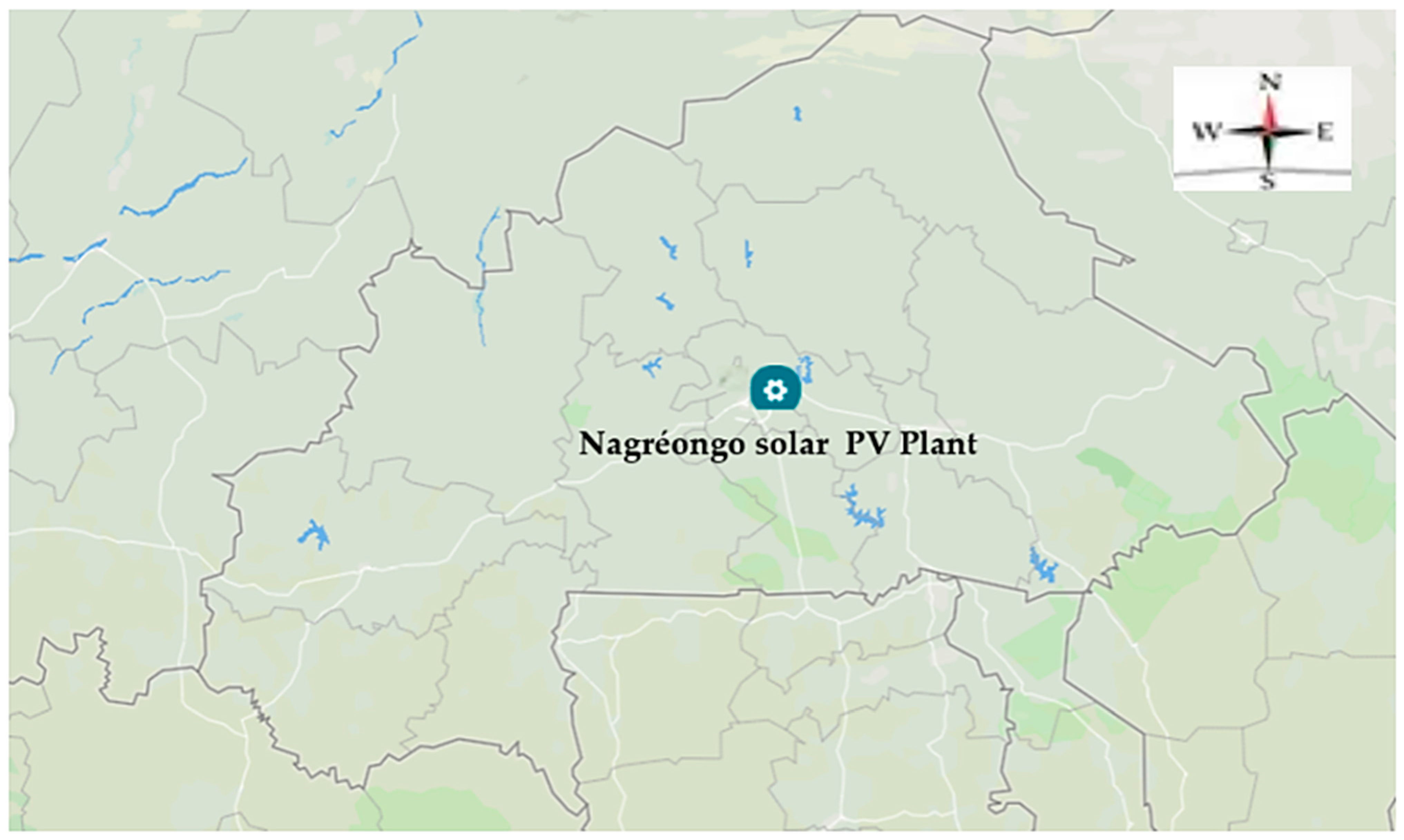
Figure 1. Nagréongo solar plant location on Burkina Faso map.
Energies 18 05285 g001
Figure 2. Overview of Nagréongo solar PV plant [22].
Energies 18 05285 g002
Figure 3. Architecture of a standard RNN [30].
Energies 18 05285 g003
Figure 4. Structure of a standard LSTM cell [37].
Energies 18 05285 g004
Figure 5. Architecture of a GRU cell [37].
Energies 18 05285 g005
Figure 6. Evolution of daily PV power over time for (a) January and February; (b) March and April; and (c) July and August over the 2024 period.
Energies 18 05285 g006
Figure 7. Flowchart of the method explaining the process of the deep learning models implemented.
Energies 18 05285 g007
Figure 8. Monthly performance ratio in (a) 2023 and (b) 2024.
Energies 18 05285 g008
Figure 9. Energy produced and losses per category in 2023.
Energies 18 05285 g009
Figure 10. Energy produced and losses per category in 2024.
Energies 18 05285 g010
Figure 11. Planned PR ratio compared to the budgeted PR.
Energies 18 05285 g011
Figure 12. Regulation losses over the past 2 years.
Energies 18 05285 g012
Figure 13. Evolution of training and validation losses with epoch for the (a) LSTM, (b) GRU, (c) LSTM-GRU, and (d) RNN models using January and February data.
Energies 18 05285 g013aEnergies 18 05285 g013b
Figure 14. Evolution of training and validation losses with epoch for the (a) LSTM, (b) GRU, (c) LSTM-GRU, and (d) RNN models using March and April data.
Energies 18 05285 g014aEnergies 18 05285 g014b
Figure 15. Evolution of training and validation losses with epoch for the (a) LSTM, (b) GRU, (c) LSTM-GRU, and (d) RNN models using July and August data.
Energies 18 05285 g015aEnergies 18 05285 g015b
Figure 16. Evolution of the daily actual and predicted PV power during the (a) dry, (b) hot, and (c) rainy seasons in the Nagréongo solar PV Plant.
Energies 18 05285 g016aEnergies 18 05285 g016b
Table 1. Summary table for data management in the performance study.
Suggested Criteria for Flag (15 min Data)
Flag TypeDescriptionIrradiance (W/m2)Temperature (°C)Wind Speed (m/s)Power
(AC Power Rating)
RangeValue outside of reasonable bounds<−6
or >1500
<−30 or >50<0 or >32<−0.01× rating
or
>1.02× rating
MissingValues missing or duplicatedn/an/an/an/a
DeadValues stuck to a single value over time; detected using derivative<0.0001
The value is >5
<0.0001??
Abrupt ChangeValues change unreasonably between data points>800>4>10>80% rating
May be adjusted depending on the tilt of the system and the season of data acquisition.
Table 2. Normal ranges of performance metrics for deep learning in PV power forecasting.
MetricExcellentGoodAcceptableWeakReference Studies
nRMSE (%)≤5%5–10%10–15%>15%[44,45,46]
nMAE (%)≤4%4–8%8–12%>12%[46]
R2 (Coefficient)≥0.950.90–0.950.80–0.90<0.80[46]
Table 3. Details of all the hyperparameters used to run the deep learning models.
CategoryHyperparameterRNNLSTMGRUHybrid LSTM–GRU
DataScaling range (0, 1)(0, 1)(0, 1)(0, 1)
Train/test split80%/20%80%/20%80%/20%80%/20%
ModelRecurrent layer 1 unitsRNN (100, return = True)LSTM (100, return = True)GRU (100, return_seq = True)LSTM (100, return_seq = True)
Dropout (after layer 1)0.20.20.20.2
Recurrent layer 2 unitsRNN (100, return_seq = False)LSTM (100, return_seq = False)GRU (100, return_seq = False)GRU (100, return_seq = False)
Dropout (after layer 2)0.20.20.20.2
Dense layer 1 units50505050
Dense layer 2 units1111
TrainingOptimiserAdam (lr = 0.001 default)Adam (lr = 0.001)Adam (lr = 0.001)Adam (lr = 0.001)
Loss functionMean squared error (MSE)MSEMSEMSE
Batch size256256256256
Epochs200200200200
Validation split0.20.20.20.2
CallbacksEarly stopping monitorval_lossval_lossval_lossval_loss
Early stopping patience10101010
Restore best weightsTrueTrueTrueTrue
Reduce LR on plateau monitorval_lossval_lossval_lossval_loss
Factor0.50.50.50.5
Patience5555
Min learning rate0.00010.00010.00010.0001
Table 4. Performance evaluation of deep learning models for the Nagreongo 30 MW PV plant during different seasons.
PeriodModelTrain RMSE (kW)Train MAE (kW)Train R2Test RMSE (kW)Test MAE (kW)Test R2nRMSE (% of 30 MW)nMAE (% of 30 MW)
Jan–FebGRU1098.69465.860.98301290.38531.630.97764.30%1.77%
Jan–FebLSTM-GRU1108.23486.410.98281293.21552.660.97754.31%1.84%
Jan–FebLSTM1133.52496.270.98201335.13570.390.97514.45%1.90%
Jan–FebRNN1132.58519.550.98201362.35598.660.97514.54%2.00%
Mar–AprGRU1075.18378.870.9810625.53271.730.99372.09%0.91%
Mar–AprLSTM-GRU1084.99407.590.9806625.51293.800.99362.09%0.98%
Mar–AprLSTM1071.46372.750.9811617.68260.330.99382.06%0.87%
Mar–AprRNN1100.86421.360.9800627.79298.310.99362.09%0.99%
Jul–AugGRU1565.38697.630.95241641.21725.650.94585.47%2.42%
Jul–AugLSTM-GRU1563.64685.930.95251646.79723.080.94545.49%2.41%
Jul–AugLSTM1564.10701.860.95251644.65734.100.94565.48%2.45%
Jul–AugRNN1567.97711.470.95231652.24746.790.94515.51%2.49%
Disclaimer/Publisher’s Note: The statements, opinions and data contained in all publications are solely those of the individual author(s) and contributor(s) and not of MDPI and/or the editor(s). MDPI and/or the editor(s) disclaim responsibility for any injury to people or property resulting from any ideas, methods, instructions or products referred to in the content.