Abstract
Accurate prediction of photovoltaic performance hinges on resolving the electron density in the P-region and the hole density in the N-region. Motivated by this need, we present a comprehensive assessment of a meshless global radial basis function (RBF) collocation strategy for the steady current continuity equation, covering a one-dimensional two-region P–N junction and a two-dimensional single-region problem. The study employs Gaussian (GA) and generalized multiquadric (GMQ) bases, systematically varying shape parameter and node density, and presents a detailed performance analysis of the meshless method. Results map the accuracy–stability–computation-time landscape: GA achieves faster convergence but over a narrower stability window, whereas GMQ exhibits greater robustness to shape-parameter variation. We identify stability plateaus that preserve accuracy without severe ill-conditioning and quantify the runtime growth inherent to dense global collocation. A utopia-point multi-objective optimization balances error and computation time to yield practical node-count guidance; for the two-dimensional case with equal weighting, an optimum of 19 intervals per side emerges, largely insensitive to the RBF choice. Collectively, the results establish global RBF collocation as a meshless, accurate, and systematically optimizable alternative to conventional mesh-based solvers for high-fidelity carrier-density prediction in P-N junctions, thereby enabling more reliable performance analysis and design of photovoltaic devices.
1. Introduction
Photovoltaic (PV) cells convert incident solar radiation into electrical power through carrier generation, separation, and collection in a semiconductor P-N junction. Central to predicting device performance is the accurate determination of the minority- and majority-carrier density profiles—the electron density in the P-region and the hole density in the N-region—particularly within the quasi-neutral regions (QNRs) on either side of the depletion layer [1,2]. These profiles control the diffusive components of the short-circuit current, set the recombination fluxes at the depletion edges, and influence the quasi-Fermi level splitting that governs open-circuit voltage and the fill factor [2]. Small errors in electron and hole densities propagate nonlinearly into the current–voltage characteristics, leading to biased estimates of key material/device parameters such as diffusion length, surface recombination velocity, and absorption coefficient. Consequently, numerical solvers that can reproduce carrier densities with high fidelity in both the P- and N-type QNRs are essential for reliable device design, parametric studies, and model-based optimization.
The carrier concentrations of a PV cell can be determined analytically [3,4,5,6,7]; however, such solutions are limited to idealized cases. Therefore, the use of numerical methods is essential for practical problems. There is a vast literature on the modeling of semiconductor devices, and the conventional methods, i.e., the finite element method (FEM), boundary element method, and finite difference method, have been applied for numerical solutions [8]. Also, simulation approaches for crystalline-Si [9], cadmium sulfide/copper zinc tin sulfide [10], perovskite [11], and organic [12] PV cells are reviewed in recent papers. While mature and accurate, mesh-based solvers typically require meshing, re-meshing, and careful stabilization, which can complicate parametric sweeps and multi-physics integrations.
Meshless methods emerged as a new class of numerical methods in the 1970s, when smoothed particle hydrodynamics [13] was introduced to tackle astrophysics problems. These methods are classified into three major groups: strong-form, weak-form, and hybrid techniques. Weak-form meshless methods are based on the weighted residual statement, where the governing differential equation is first integrated over the problem domain, and the formulation depends on the choice of shape and weight functions. Weak-form methods necessitate the use of an inherent background mesh for numerical integration, and therefore are not truly meshless. On the contrary, shape functions are directly substituted into the governing equation in strong-form approaches, and there is no need for integration. Hybrid methods combine the strong- and weak-form approaches to take advantage of the superior features of both classes.
The radial basis function (RBF) collocation method is a strong-form meshless method. It was proposed by Kansa [14] to solve hydrodynamics problems, and since its introduction, the method has found a large application area in various branches of science, including heat transfer [15], fluid dynamics [16], quantum physics [17], and neutron transport [18]. Although RBFs are theoretically more stable when they are used within a weak-form sense [19], the RBF collocation method is advantageous to both conventional mesh-based and alternative meshless methods with its exponential convergence rate and ease of implementation. The original version of the RBF collocation proposed by Kansa is a global method in which all interpolation nodes are utilized in approximating the field variable in a certain location, and the resultant collocation matrix is full. However, the method can also be implemented in a local manner by defining support domains that limit the number of interpolation nodes used for approximation. The local RBF collocation method is more stable but less accurate than its global counterpart.
Meshless methods were used for modeling PV cells. The finite point method was used to solve the semiconductor Poisson equation [20], and the method showed good agreement with the finite difference solution for two- and three-dimensional problems. Kosec and Trobec [21] used the local RBF collocation method to tackle a P-N junction problem with the drift diffusion model. A refinement strategy was used to decrease the number of nodes required for adequate convergence, and numerical tests were carried out to demonstrate the applicability of the method for different cases. The global RBF collocation method was used to model a one-dimensional gallium arsenide (GaAs) solar cell [22]. However, the analysis fixed a single node set and a single shape parameter, precluding a systematic examination of accuracy–stability trade-offs and offering limited guidance on how basis selection, shape parameter, and node density affect the fidelity of electron and hole density fields in the P and N regions. A physics-informed deep learning approach is proposed by [23] to obtain meshless solutions for semiconductor devices. In another recent study [24], a hybrid collocation-mixed FEM is introduced to model flexoelectricity and electron transport in semiconductors.
The literature review shows that there exists no detailed analysis on the use of the global RBF collocation method for the numerical modeling of PV cells. Therefore, prior literature does not distill actionable defaults—i.e., ready-to-use prescriptions that tie basis selection to operating regimes, specify shape-parameter windows that balance accuracy and conditioning, and quantify node-density targets for reproducible error tolerances. This study fills that gap by presenting a comprehensive assessment of the meshless global RBF collocation method for the time-independent current continuity equation in one-dimensional two-region and two-dimensional single-region PV problems. We analyzed (i) the one-dimensional P-N junction, with targeted parametric studies on surface recombination velocity, diffusion length, and absorption coefficient to stress the solver’s ability to recover accurate electron and hole densities in the QNRs and (ii) the two-dimensional single-region case to quantify accuracy in multidimensional transport against a high-fidelity FEM reference. Gaussian (GA) and generalized multiquadric (GMQ) bases are used as the RBFs, and the effects of interpolation node density and shape parameter on the performance of the RBF collocation method are studied in detail.
The work provides, to the best of our knowledge, the first systematic, device-focused map of accuracy, stability, and computation cost for global RBF collocation in PV transport, delivering the following:
- (1)
- A side-by-side comparison of GA and GMQ bases across wide shape parameter and node density ranges;
- (2)
- Stability windows and near-optimal plateaus that practitioners can use to select basis/parameter pairs that preserve accuracy in the P- and N-region QNRs without incurring ill-conditioning;
- (3)
- A multi-objective optimization framework that balances error against central processing unit (CPU) time and yields practical node-count guidelines;
- (4)
- Actionable best-practice recommendations (basis selection, shape-parameter tuning, and conditioning strategies) that translate directly to PV modeling workflows.
In this work, the device physics is restricted to the current continuity equation within the QNRs, where the electric field is zero. Also, there are no explicit bulk Shockley–Read–Hall, radiative, or Auger recombination terms in the solved differential equations, and recombination enters through surface recombination velocities at the depletion edges. As such, we do not aim to reproduce a full-device solution of the coupled drift–diffusion–Poisson system that is often required for predictive design and calibration. Instead, our contribution is methodological: we map the accuracy–stability–computation-time landscape of global RBF collocation for transport-type operators relevant to PV modeling and provide guidance on basis/shape-parameter/node-density choices.
The remainder of the paper is organized as follows. Section 2 formulates the steady-state carrier continuity equation for the P- and N-type QNRs of a one-dimensional P–N junction and for a two-dimensional single-region problem. Section 3 presents the global RBF collocation methodology, detailing the basis functions and implementation of the method for the carrier continuity equation. Section 4 presents the results of the study, and the paper is concluded in Section 5.
2. Current Continuity Equations for a PV Cell
The current continuity equation plays a key role in the drift-diffusion model of a semiconductor device and has the following general form [25]:
where is the diffusion coefficient, is the charge density, and are functions that are independent of , is the electrostatic potential, represents the domain, and and represent the Dirichlet and Neumann boundaries, respectively.
For a two-dimensional single-region problem in Cartesian geometry, Equation (1) takes the following form if has a constant gradient of , and homogeneous Dirichlet boundary conditions exist on all boundaries of the domain:
An explicit model can be given for a one-dimensional two-region problem in Cartesian geometry. The current continuity equations for the P and N regions of a P-N junction are [26]
where is the electron density in the P region, is the hole density in the N region, is the mobility, is the diffusion length, is the electric field, is the photogeneration rate, and and are the equilibrium densities of and , respectively. Photogeneration rates of the P and N regions are determined by
where is the absorption coefficient, is the photon flux, and are the P and N depletion region depths, respectively, and and are boundaries of the P and N regions, respectively, (see Figure 1). The boundary conditions complementing the model are
where and are the surface recombination velocities of P and N regions, respectively.
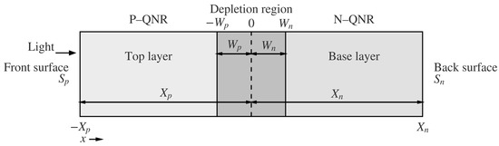
Figure 1.
Schematic representation of the photovoltaic cell (adapted from [23]).
Since the electric field is assumed to be zero in the QNR, Equation (3) simplifies to
Accurate calculation of electron and hole densities is critical in determining the performance metrics of the PV. The current density is computed by
where is the electron charge. Current density is used to determine the short-circuit and open-circuit points, and the power delivered by the PV. Consequently, the fill factor and power conversion efficiency of the device are smooth functionals of and hence carrier densities.
3. Radial Basis Function Collocation Method
Radial basis functions are kernel functions that enable meshless approximation on scattered data, independently of the spatial dimension. An RBF depends solely on the Euclidean distance, , between the center and the evaluation point. Numerous RBFs exist in the literature, and their characteristics are studied in detail [27]. In this work, GMQ and GA RBFs are used for the collocation solution of the current continuity equation to model the carrier distribution in a PV cell:
In Equation (8), is referred to as the shape parameter and has a significant impact on the accuracy and stability of the RBF collocation method. In the case of function interpolation, larger values of tend to improve the accuracy of the approximation for the sake of ill-conditioning and hence decrease the stability of the method [28]. A similar behavior is also observed for the RBF collocation solution of PDEs [29]; however, the ill-conditioning problem can be overcome by increasing the precision of computation [30], optimization of the shape parameter [31], or matrix preconditioning [32]. The exponent of the GMQ, , has an effect that is similar to the impact of on the performance of the RBF collocation method. A larger is preferable in terms of accuracy; however, increasing also decreases the stability of the method. GMQ is referred to as the multiquadric (MQ) and inverse multiquadric (IMQ) when is chosen to be and , respectively.
The formulation of the RBF collocation method will be explained through the two-dimensional current continuity equation. The numerical solution begins by approximating the dependent variable with a finite series of RBFs:
where is the total number of domain, boundary, and external nodes, is the coefficient to be determined and has the following explicit form in two-dimensional Cartesian geometry:
External nodes are utilized to improve the accuracy of the method near the boundaries by collocating the differential equation on both the domain and boundary nodes.
The second step of the numerical solution involves the substitution of Equation (9) into Equation (2) and collocating the resultant equations on the collocation nodes :
where and are the number of domain and boundary nodes, respectively, and
Equation (11) is an system of algebraic equations, the solution of which yields , and hence the numerical approximation.
In this work, stability refers to the numerical conditioning of the collocation matrix, , and is quantified by the spectral condition number defined as [33]
where and are the maximum and minimum singular values of the collocation matrix, respectively. The condition number measures the sensitivity of the discrete solution to perturbations from data noise and round-off.
4. Results and Discussion
The performance of the global RBF collocation method in solving the current continuity equation is assessed through two cases. First, a one-dimensional two-region problem is studied in detail by considering the impacts of surface recombination rate, diffusion length, and absorption coefficient on the characteristics of the numerical solutions. The second problem is a two-dimensional single region case where a multi-objective optimization is performed to determine the optimum number of interpolation nodes to simultaneously optimize the accuracy and computation time of the RBF collocation method, since for two-dimensional problems, the computation time becomes a critical factor due to the fully populated structure of the collocation matrix. All calculations are performed with in-house codes developed with Mathematica 11. In order to demonstrate the full potential of the RBF collocation, arbitrary precision arithmetic is utilized with 200-precision for the one-dimensional problem. However, the use of high precision significantly increases the CPU time for two-dimensional cases, and hence, the machine precision of Mathematica, which is approximately equivalent to double-precision arithmetic, is used for the two-dimensional problem. The accuracy of the meshless approach is determined by calculating the root mean square (rms) and maximum errors:
where and denote the reference and numerical solution, respectively.
4.1. One-Dimensional Two-Region Problem
The first problem is the one-dimensional two-region case for which the analytical solution can be found in [34]. The physical parameters are selected as , , , , and , unless they are considered as a variable in numerical tests. The surface recombination rate has a noticeable impact on carrier densities, as illustrated in Figure 2. The electron density decreases significantly in the range as the recombination rate increases from to . Therefore, RBF collocation solutions are obtained for and .
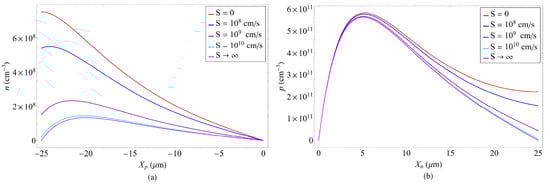
Figure 2.
Effect of surface recombination rate on (a) electron and (b) hole carrier densities.
Figure 3 shows the variation of and with respect to the shape parameter in the range for and . These results are obtained with , and the recombination rate is chosen to be to represent the case, since density distributions become insensitive to above this value. The high-level accuracy of GMQ improved with increasing , and good stability is observed for all exponent values. Although the error of GA increases with increasing , GA collocation still provides a high accuracy for all cases. This basis function provides higher accuracy and converges faster than GMQ when . The stability plateaus of all basis functions, the minimum error values, and condition numbers that correspond to the upper limit of the stable range are presented in Table 1. The limiting values are the shape parameters, where a slight increment is observed in rms and maximum errors.
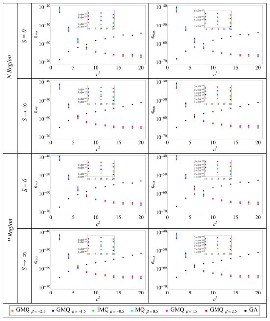
Figure 3.
Shape parameter convergence of GMQ and GA for electron and hole densities in cases of and with where collocation is performed with .

Table 1.
Shape parameter stability limits and corresponding error and condition numbers for the one-dimensional problem.
The variation in the condition number with the shape parameter for all basis functions is illustrated in Figure 4. The safe limit for the condition number, , is reached for the GMQ at ; however, as Table 1 indicates, the collocation method converges smoothly up to for . Such behavior is also observed for the Poisson equation [35]. On the other hand, GA becomes unstable at at which also reaches the ill-conditioning limit.
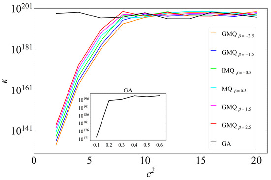
Figure 4.
Variation of with for GMQ and GA, where collocation is performed with .
The number of interpolation nodes employed in the RBF collocation solution of the current continuity equation affects the modeling, as shown in Figure 5, where . The method converges smoothly with for both regions and recombination rate values for all basis functions. Overall, increasing the exponent of GMQ improves its error behavior. The accuracy of GA is superior to GMQ when ; however, for large values, the error values become identical for both basis functions. Also, the GA function converges faster than GMQ for sparse sets of interpolation nodes.
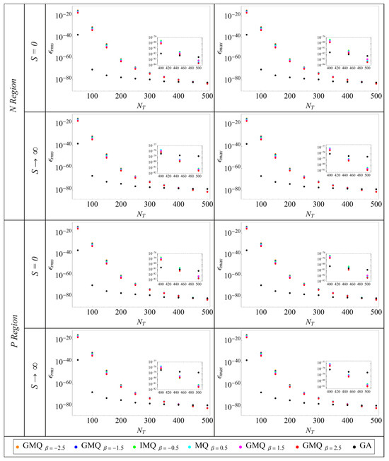
Figure 5.
Interpolation node number convergence of GMQ and GA for electron and hole densities in cases of and with where .
Similar to the surface recombination rate, diffusion length and absorption coefficient also have a major effect on PV cell modeling. Carrier density distributions in the P and N regions calculated with different diffusion lengths using an surface recombination rate are plotted in Figure 6. An increment of in the diffusion length from to triples the electron and hole densities. The impact of absorption coefficient on the spatial distribution of carrier densities is illustrated in Figure 7, where it is clear that has a significant effect on the hole density distribution.
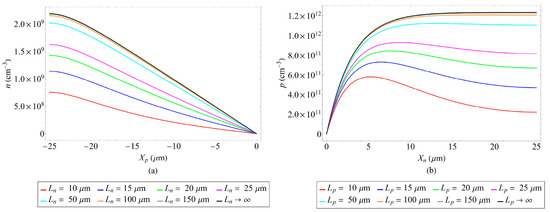
Figure 6.
Carrier density distributions for various (a) and (b) values, where .
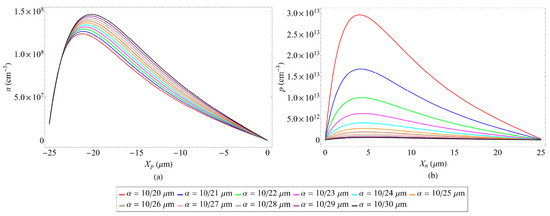
Figure 7.
Impact of absorption coefficient on (a) electron and (b) hole carrier densities, where .
To test the robustness of the global RBF collocation method, calculations are performed for and , and the results showing the node number convergence of the meshless algorithm are presented in Figure 8 and Figure 9, respectively, where the shape parameter is chosen as . Diffusion lengths of are assumed to represent the case. A comparison with the convergence curves of Figure 4 reveals that similar error behavior is present for all RBFs in both N and P regions and surface recombination rates. Increasing the value of improves the accuracy of the method, while GA collocation yields the best convergence rate for sparse node configurations. The shape parameter convergence of the and cases are also studied, and the convergence curves are similar to those presented in Figure 3.
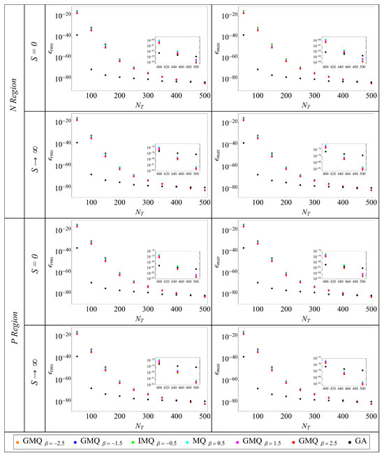
Figure 8.
Interpolation node number convergence of GMQ and GA for electron and hole densities in cases of and with where .
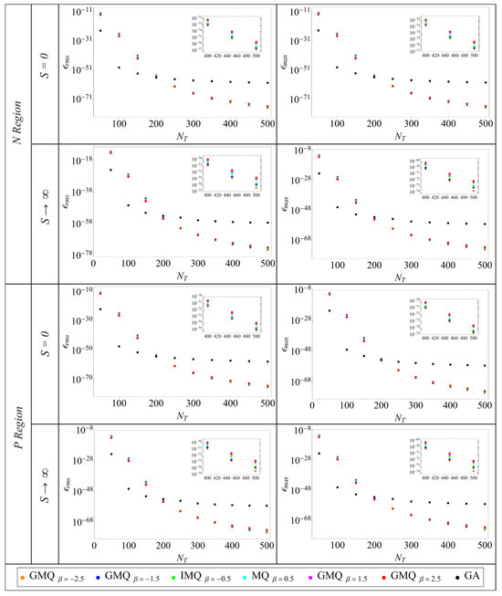
Figure 9.
Interpolation node number convergence of GMQ and GA for electron and hole densities in cases of and with where .
The accuracy of the meshless method is further illustrated in Figure 10 through the comparison of analytical and numerical solutions for , , and where . RBF collocation solution is obtained with the MQ basis function employing and . Results clearly show that the numerical electron, hole, and current densities exactly match the analytical solutions.
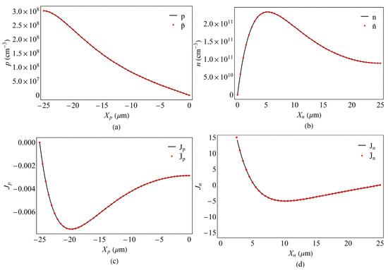
Figure 10.
Comparison of analytical and numerical electron, hole, and current densities for the one-dimensional problem. (a) Hole density; (b) Electron density; (c) Hole current density; (d) Electron current density.
4.2. Two-Dimensional Single Region Problem
The two-dimensional current continuity equation, Equation (2), is solved with , , , [25] on a domain of the unit square. This problem does not have an analytical solution, and to evaluate the performance of the global RBF collocation method, FEM is applied to Equation (2). Triangular finite elements are used within the solution, and the FEM solver of Mathematica’s built-in function NDSolve is utilized for computations. Maximum mesh length, , has a significant impact on the solution as observed from the FEM solutions obtained with various maximum mesh lengths illustrated in Figure 11 and Figure 12. Based on these results, the FEM solution with , which minimizes the oscillatory behavior near the boundaries, is chosen as the reference solution of the two-dimensional single region problem. The high fidelity of the numerical solution employing is obvious from Figure 12b, where it is seen that numerical artifacts (i.e., numerical values larger than 1) that are quantified by vanish completely when .
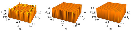
Figure 11.
FEM solutions of the two-dimensional problem where , , , obtained with maximum mesh lengths of (a) , (b) , (c) .
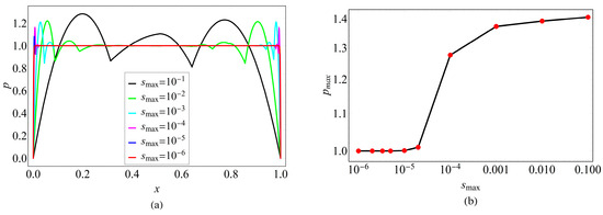
Figure 12.
Impact of on the FEM solution of the 2D problem: (a) oscillatory behavior is observed for when is large. (b) Numerical artifacts vanish when .
Shape-parameter convergence curves of the global RBF collocation solution to the two-dimensional problem are presented in Figure 13, where the number of intervals per side is (i.e., ). GMQ demonstrates good stability in the given shape parameter range, and similar convergence rates are found for all exponent values. Also, a larger is preferable for better accuracy. As for the GA, the meshless collocation method is stable in the range , converges faster than GMQ in the stable computation region, and produces more accurate results when . It should also be noted that due to the use of machine precision arithmetic, the accuracy level observed for the two-dimensional problem is low compared to the results presented for the one-dimensional case.
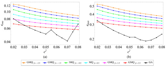
Figure 13.
Variation in (a) and (b) with for the two-dimensional problem, where , , , .
The impact of on the accuracy of the RBF collocation method is shown in Figure 14 for four values of the shape parameter. The method produced accurate results for all values of in a stable manner. GA dominates GMQ with its faster convergence rate as the number of interpolation nodes increases, and the advantage of GA becomes more apparent as the shape parameter increases. The results also reveal that the convergence rate of GMQ is insensitive to . The hole density distributions obtained with MQ, IMQ, and GA collocation are presented in Figure 15 for four sets of interpolation nodes. The global meshless method produces smooth solutions with for all basis functions. This situation can also be observed from Figure 16, which illustrates the error distribution of the MQ collocation employing and over the whole problem domain.
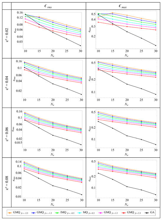
Figure 14.
Variation of and with and for the two-dimensional problem, where , , , .
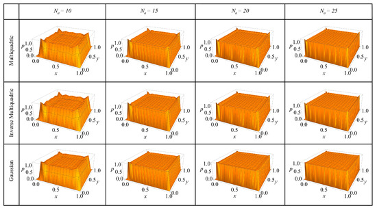
Figure 15.
Hole density distributions for the two-dimensional problem calculated with MQ, IMQ, and GA collocation employing , where , , , .
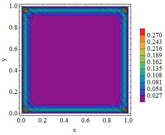
Figure 16.
Error map for the two-dimensional problem, where , , , . MQ collocation is performed with and .
Computation time becomes a critical issue when the global RBF collocation method is used for two- and three-dimensional problems, since the collocation matrix is fully populated. This issue is illustrated in Figure 17, where the CPU-time–node-number relationship is plotted for the RBF collocation solution of the two-dimensional problem. Computation time increases in a fast manner with increasing , and depending on the choice of radial function, CPU times exceed 5000 s when These results indicate that there is a conflicting trend among the accuracy and computation time of the global RBF collocation method. Therefore, a multi-objective optimization is performed to determine the optimum value of that simultaneously optimizes accuracy and CPU time of the meshless approach for two-dimensional problems. Optimization is carried out with the utopia-point method, in which a composite function is minimized
where represents the objective function, is the decision variable, is an integer, which is usually taken as 2 to denote the Euclidean distance between the utopia () and actual values of the objective functions, and is the weight of the objective function. Equation (15) takes the following form for the RBF collocation method:
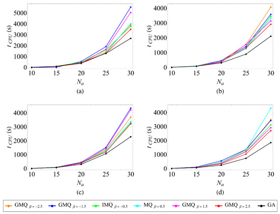
Figure 17.
Variation in RBF collocation CPU time with for (a) , (b) , (c) , and (d) .
To determine the optimum number of interpolation nodes for the RBF collocation method, the values corresponding to different are first computed, and subsequently, quadratic polynomials are constructed with Mathematica for various values of the shape parameter. Optimum values that minimize the composite objective function are given in Table 2. is found to be relatively insensitive to the choice of RBF and shape parameter. When equal importance is given to accuracy and CPU time (i.e., ), the optimum value of is 19 for most of the RBF–shape parameter alternatives. Numerical tests with IMQ revealed that moving from to (i.e., nodes) raised CPU time from to —an 8.85-fold increase—with only marginal accuracy gains. Conversely, (i.e., 121 nodes) finished in ( of the CPU time) but doubled the fill distance, which visibly increases discretization errors. These data justify the utopia point near ; accuracy has largely saturated, yet computational cost still rises steeply beyond this setting. The results of Table 2 also show that and decrease with a decrease in , indicating that the CPU time is much more influenced by interpolation node density as compared to the accuracy.
Table 2.
and calculated for GMQ and GA with different values of and .
The two-dimensional problem is solved with (i) a diffusion-dominated setting of and (ii) homogeneous Neumann boundary conditions on the left and bottom edges (Dirichlet on the remaining edges) to assess the effects of physical parameters and boundary conditions on the multi-objective optimization. Applying the same utopia-point procedure again selected when equal weighting of accuracy and computation time is considered. However, these results should not be interpreted as a universal setting of , since irregular three-dimensional geometries can alter CPU time growth and convergence rates of the RBF collocation method.
5. Conclusions
This study presented and rigorously assessed a global RBF collocation framework for modeling carrier transport in PV cells. Two cases, a one-dimensional two-region and a two-dimensional single-region problem, are modeled with the meshless method, where GMQ with various exponents and GA are used as the radial functions. Effects of interpolation node density and shape parameter on the performance of the method are analyzed. By solving the current continuity equations in both a one-dimensional P-N junction and a two-dimensional single-region setting, we quantified how algorithmic choices—basis type, shape parameter, and interpolation node density—govern accuracy, stability, and computational cost. The main findings of this study are as follows:
- The global RBF collocation method accurately reproduces carrier distributions in one-dimensional P-N junctions and two-dimensional domains, confirming its suitability for semiconductor device modeling.
- Basis selection matters: GA basis typically exhibits faster convergence and lower errors at comparable node counts but over a narrower stability window; GMQ variants are more robust to shape-parameter variation, albeit with slightly slower convergence.
- Shape parameter critically affects both error and conditioning; stable plateaus exist where accuracy is near-optimal without severe ill-conditioning, while an overly large shape parameter can destabilize GA in particular.
- Because the collocation matrix is dense, CPU time rises rapidly with node count. A utopia-point multi-objective optimization that balances error and runtime yields practical design guidance: for the 2D problem considered, an optimum of 19 intervals per side (equal weights on accuracy and CPU time) gives a near-Pareto solution, largely insensitive to the specific RBF choice.
- Physically, the meshless solver captures the expected sensitivities of carrier densities to surface recombination velocity, diffusion length, and absorption coefficient, aligning with analytical trends and reinforcing the model’s predictive value.
In addition to these results, it should also be noted that for practitioners seeking a robust default, the inverse multiquadric basis is a strong baseline in global RBF collocation: it delivers stable performance with moderate sensitivity to the shape parameter, and it integrates cleanly with oversampled least-squares solvers.
The present findings can be used as a drop-in strong-form transport solver within standard drift–diffusion–Poisson iterations and opto–electro–thermal co-simulations by replacing mesh generation with node placement and choosing shape parameters inside the reported stability plateaus. The multi-objective optimization algorithm can be implemented to determine the optimum node setting for desired accuracy and computation time. In commercial codes that are primarily FEM-based, the RBF collocation step can be scripted externally to generate carrier density fields and recombination currents that are imported as tables for calibration and mesh-policy tuning, thereby reducing expensive mesh-refinement loops.
Overall, the global RBF collocation emerges as a meshless, accurate, and systematically optimizable alternative to conventional mesh-based solvers for PV modeling, providing clear guidance on basis/parameter choices and node density sizing to balance accuracy with computational efficiency. The present analysis focuses on the current continuity equation under standard assumptions. Future extensions may integrate non-uniform doping and bias-dependent depletion widths, and recombination mechanisms (Shockley–Read–Hall, radiative, Auger) in multi-region two-dimensional geometries. Also, coupling with optical models (spectral photogeneration) and temperature-dependent transport will enable end-to-end PV performance prediction and design optimization.
While the two-region problem highlights the cost of dense global collocation in multidimensional cases, several remedies, such as domain decomposition, compactly supported RBFs, and acceleration with fast multipole method or fast Gauss transform, can improve the computation time without sacrificing accuracy. The results of this study can be viewed as a baseline for these strategies; future work can port the safe shape-parameter/node-density regimes identified here into solvers employing these approaches. Also, the global RBF collocation framework can be transferred directly to three dimensions by replacing planar node sets with volumetric node clouds that resolve junction curvature and steep doping/field gradients.
Author Contributions
Conceptualization, T.T.; methodology, T.T.; software, M.I. and T.T.; validation, M.I.; formal analysis, M.I.; investigation, M.I.; resources, T.T.; data curation, M.I.; writing—original draft preparation, M.I. and T.T.; writing—review and editing, T.T.; visualization, M.I.; supervision, T.T.; project administration, T.T. All authors have read and agreed to the published version of the manuscript.
Funding
This research received no external funding.
Data Availability Statement
The raw data supporting the conclusions of this article will be made available by the authors on request.
Acknowledgments
This manuscript was prepared from Murat Ispir’s study conducted at Bursa Technical University.
Conflicts of Interest
The authors declare no conflicts of interest.
Abbreviations
The following abbreviations are used in this manuscript:
| CPU | Central processing unit |
| FEM | Finite element method |
| GA | Gaussian |
| GMQ | Generalized multiquadric |
| IMQ | Inverse multiquadric |
| MQ | Multiquadric |
| PV | Photovoltaic |
| QNR | Quasi-neutral region |
| RBF | Radial basis function |
References
- Sze, S.M.; Ng, K.K. Physics of Semidoncuctor Devices, 3rd ed.; Wiley: Hoboken, NJ, USA, 2007. [Google Scholar]
- Nelson, J. The Physics of Solar Cells; Imperial College Press: Singapore, 2003. [Google Scholar]
- Velazquez-Perez, J.E.; Gurevich, Y.G. Charge-carrier transport in thin film solar cells: New formulation. Int. J. Photoenergy 2011, 2011, 976063. [Google Scholar] [CrossRef]
- Biswas, S.; Sinha, A. An analytical study of the minority carrier distribution and photocurrent of a p–i–n quantum dot solar cell based on the InAs/GaAs system. Indian J. Phys. 2017, 91, 1197–1203. [Google Scholar] [CrossRef]
- Sahin, G.; Kerimli, G. Effect of the depth base along the vertical on the electrical parameters of a vertical parallel silicon solar cell in open and short circuit. Results Phys. 2018, 8, 257–261. [Google Scholar] [CrossRef]
- Guo, M.; Li, Y.; Qin, G.; Zhao, M. Nonlinear solutions of PN junctions of piezoelectric semiconductors. Acta Mech. 2019, 230, 1825–1841. [Google Scholar] [CrossRef]
- Nihako, J.N.; Simo, E.; Essouma, D.D.A.; Leutchouang, M.N.; Tsakem, C.R.A.; Tchienou, C.Y.T.; Watia, J.S.K.; Logerais, P.O.; Djouda, J.M. Realistic modeling of photovoltaic solar cell: A simple and accurate two-diode model. Appl. Res. 2025, 4, e70010. [Google Scholar] [CrossRef]
- Snowden, C.M.; Miles, R.E. Compound Semiconductor Device Modelling; Springer: London, UK, 1993. [Google Scholar]
- Sugiura, T.; Nakano, N. Review: Numerical simulation approaches of crystalline-Si photovoltaics. Energy Sci. Eng. 2023, 11, 3888–3906. [Google Scholar] [CrossRef]
- Haddout, A.; Raidou, A.; Fahoume, M. A review on the numerical modeling of CdS/CZTS-based solar cells. Appl. Phys. A 2019, 125, 124. [Google Scholar] [CrossRef]
- Nkele, A.C.; Ike, I.S.; Ezugwu, S.; Maaza, M.; Ezema, F.I. An overview of the mathematical modelling of perovskite solar cells towards achieving highly efficient perovskite devices. Int. J. Energy Res. 2021, 45, 1496–1516. [Google Scholar] [CrossRef]
- Groves, C. Simulating charge transport in organic semiconductors and devices: A review. Rep. Prog. Phys. 2017, 80, 026502. [Google Scholar] [CrossRef]
- Lucy, L.B. A numerical approach to the testing of the fission hypothesis. Astron. J. 1977, 82, 1013–1024. [Google Scholar] [CrossRef]
- Kansa, E.J. Application of Hardy’s Multiquadric Interpolation to Hydrodynamics. In Proceedings of the 1986 Summer Computer Simulation Conference, San Diego, CA, USA, 23–25 January 1986; Crosbie, R., Luker, P., Eds.; Society for Computer Simulation: San Diego, CA, USA, 1986; Volume 4, pp. 111–117. [Google Scholar]
- Jamil, M.; Ng, E.Y.K. Evaluation of meshless radial basis collocation method (RBCM) for heterogeneous conduction and simulation of temperature inside biological tissues. Int. J. Therm. Sci. 2013, 68, 42–52. [Google Scholar] [CrossRef]
- Waters, J.; Pepper, D.W. Global versus localized RBF meshless methods for solving incompressible fluid flow with heat transfer. Numer. Heat Transf. B 2015, 68, 185–203. [Google Scholar] [CrossRef]
- Karabaş, N.İ.; Korkut, S.Ö.; Tanoğlu, G.; Aziz, I.; Islam, S. An efficient approach for solving nonlinear multidimensional Schrödinger equations. Eng. Anal. Bound. Elem. 2021, 132, 263–270. [Google Scholar] [CrossRef]
- Tanbay, T.; Ozgener, B. Fully meshless solution of the one-dimensional multigroup neutron transport equation with the radial basis function collocation method. Comput. Math. Appl. 2020, 79, 1266–1286. [Google Scholar] [CrossRef]
- Duan, Y. A note on the meshless method using radial basis functions. Comput. Math. Appl. 2008, 55, 66–75. [Google Scholar] [CrossRef]
- Wordelman, C.J.; Aluru, N.R.; Ravaioli, U. A meshless method for the numerical solution of the 2- and 3-D semiconductor Poisson equation. CMES Comput. Model. Eng. Sci. 2000, 1, 121–126. [Google Scholar] [CrossRef]
- Kosec, G.; Trobec, R. Simulation of semiconductor devices with a local numerical approach. Eng. Anal. Bound. Elem. 2015, 50, 69–75. [Google Scholar] [CrossRef]
- Kinani, M.; Amine, A.; Mir, Y.; Zazoui, M. A numerical study of InGaAs/GaAsP multiple quantum well solar cells using radial basis functions. In Proceedings of the 2nd International Conference on Electronic Engineering and Renewable Energy Systems, Saidia, Morocco, 2–4 April 2020; Hajji, B., Mellit, A., Tina, G.M., Rabhi, A., Launay, J., Naimi, S.E., Eds.; Springer: Singapore, 2021; Volume 681, pp. 231–238. [Google Scholar]
- Riganti, R.; Alasio, M.G.C.; Bellotti, E.; Dal Negro, L. DDNet: A unified physics-ınformed deep learning framework for semiconductor device modeling. arXiv 2025. [Google Scholar] [CrossRef]
- Tian, X.; Zhou, H.; Hu, Y.; Deng, Q.; Xu, M.; Sladek, J.; Sladek, V.; Shen, S. Nonlinear interaction studies of flexoelectricity and electron transport around nano-cracks in semiconductors via the collocation mixed finite element method. J. Appl. Phys. 2025, 137, 194103. [Google Scholar] [CrossRef]
- Brezzi, F.; Marini, L.D.; Micheletti, S.; Pietra, P.; Sacco, R.; Wang, S. Discretization of semiconductor device problems (I). Handb. Numer. Anal. 2005, 13, 317–441. [Google Scholar] [CrossRef]
- Archer, M.D.; Bolton, J.R.; Siklos, S.T.C. A review of analytic solutions for a model p–n junction cell under low-injection conditions. Sol. Energy Mater. Sol. Cells 1996, 40, 133–176. [Google Scholar] [CrossRef]
- Buhmann, M.D. Radial Basis Functions: Theory and Implementations; Cambridge University Press: Cambridge, UK, 2003. [Google Scholar] [CrossRef]
- Schaback, R. Error estimates and condition numbers for radial basis function interpolation. Adv. Comput. Math. 1995, 3, 251–264. [Google Scholar] [CrossRef]
- Tanbay, T.; Ozgener, B. A comparison of the meshless RBF collocation method with finite element and boundary element methods in neutron diffusion calculations. Eng. Anal. Bound. Elem. 2014, 46, 30–40. [Google Scholar] [CrossRef]
- Huang, C.-S.; Lee, C.-F.; Cheng, A.H.-D. Error estimate, optimal shape factor, and high precision computation of multiquadric collocation method. Eng. Anal. Bound. Elem. 2007, 31, 614–623. [Google Scholar] [CrossRef]
- Luh, L.T. The choice of the shape parameter—A friendly approach. Eng. Anal. Bound. Elem. 2019, 98, 103–109. [Google Scholar] [CrossRef]
- Kansa, E.J.; Hon, Y.C. Circumventing the ill-conditioning problem with multiquadric radial basis functions: Applications to elliptic partial differential equations. Comput. Math. Appl. 2000, 39, 123–137. [Google Scholar] [CrossRef]
- Cheng, A.H.-D. Multiquadric and its shape parameter-A numerical investigation of error estimate, condition number, and round-off error by arbitrary precision computation. Eng. Anal. Bound. Elem. 2012, 36, 220–239. [Google Scholar] [CrossRef]
- Fahrenbruch, A.; Bube, R. Fundamentals of Solar Cells: Photovoltaic Solar Energy Conversion; Elsevier: Amsterdam, The Netherlands, 2012. [Google Scholar]
- Cheng, A.H.-D.; Golberg, M.A.; Kansa, E.J.; Zammito, G. Exponential convergence and h-c multiquadric collocation method for partial differential equations. Numer. Methods Partial Differ. Equ. 2003, 19, 571–594. [Google Scholar] [CrossRef]


Disclaimer/Publisher’s Note: The statements, opinions and data contained in all publications are solely those of the individual author(s) and contributor(s) and not of MDPI and/or the editor(s). MDPI and/or the editor(s) disclaim responsibility for any injury to people or property resulting from any ideas, methods, instructions or products referred to in the content. |
© 2025 by the authors. Licensee MDPI, Basel, Switzerland. This article is an open access article distributed under the terms and conditions of the Creative Commons Attribution (CC BY) license (https://creativecommons.org/licenses/by/4.0/).