Article

Estimated Ultimate Recovery (EUR) Prediction for Eagle Ford Shale Using Integrated Datasets and Artificial Neural Networks

U.S. Geological Survey, Geology, Energy & Minerals Science Center, Reston, VA 20192, USA
*
Author to whom correspondence should be addressed.
Energies 2025, 18(19), 5216; https://doi.org/10.3390/en18195216
Submission received: 19 August 2025 / Revised: 16 September 2025 / Accepted: 24 September 2025 / Published: 30 September 2025

Abstract

The estimated ultimate recovery (EUR) is an important parameter for forecasting oil and gas production and informing decisions regarding field development strategies. In this study, we combined site-specific geologic, completion, and operational parameters with the predictive capabilities of machine learning (ML) models to predict EURs of the wells for the Eagle Ford Marl Continuous Oil Assessment Unit. We developed an extensive dataset of wells that have produced from the lower and upper Eagle Ford Shale intervals and reduced the model complexity using principal component analysis. We tested the ML models and estimated the sensitivities of ML-predicted EURs to changes in the values of different input variables. The results of applying the optimized ML model to the Eagle Ford suggest that the approach developed in this study could be promising. The ML estimates of the EURs fit the DCA-based values with an R2 ~ 0.9 and a mean absolute error of ~36 × 103 bbl. In the lower Eagle Ford Shale, the EUR estimates were found to be most sensitive to changes in porosity, net thickness of the interval, clay volume, and the API gravity of the oil; and that in the upper Eagle Ford Shale they were most sensitive to changes in the total organic carbon and water saturation, which suggests that it could be important to consider these parameters in assessing these intervals or close analogs.

1. Introduction

Production and estimated ultimate recovery (EUR) analysis of wells drilled in continuous (unconventional) accumulations of petroleum resources reveals how much and/or how quickly they could produce. Thus, EUR analysis is critical for resource assessments, and it can be useful in helping to locate the best acreage within the broader continuous resource play (often referred to as sweet spots) along with subsequent economic analysis [1,2,3].
Due to its importance, there have been several methods developed over the years to determine the EUR, i.e., production decline curve analysis (DCA), rate transient analysis (RTA), flowing material balance (FMB), and numerical simulation. The material balance method (FMB) is based on mass conservation by involving a few of the geological and fluid parameters, such as porosity and compressibility, respectively, in computations to analyze the relationship between production and formation pressure. Rate transient analysis (RTA) combines diagnostics, flow regime identification, and qualitative and quantitative interpretation for reservoir characterization and production forecasts. The application requires pressure data in addition to production data and can be tedious. Numerical simulation, on the other hand, incorporates the most advanced physics through equations describing flow, pressure, and saturations. However, it requires an extensive dataset for building the model of a certain geometry and for its validation. Both FMB and numerical simulation are independent of specific empirical models and are free from the limitations of the flow regime. In addition, numerical simulation can analyze interferences between wells that affect the EUR [4]. Extensive data and modeling requirements may come with a reward that these models can also provide the most insight into how variables such as well-completion and reservoir and fluid properties, as well as differences in reservoir settings (e.g., depth, thickness), can affect production and its decline, and therefore the EUR. Amongst all these methods, DCA is probably the most widely used one. This is owing to the ease of application, especially for many hundreds (or in some cases, thousands) of wells, and minimum data requirements beyond production history. Despite its popularity, traditional DCA can fall short of accuracy and information content due to inherent assumptions, missing reservoir signals in DCA models, ignoring the production history of other wells in the same geologic formation, or excluding a target well’s important attributes relevant to production [5]. The shortfalls of DCA can be compounded with extended transient period of shale oil and gas wells delaying boundary dominated flow period (BDF), and the common assumption that the operational parameters of the wells will continue without change in the future, which may not be a realistic expectation. Nevertheless, several analysts have developed DCA models to address some challenges posed by shale reservoir characteristics and predict the EURs of shale reservoirs [6,7], as well as for accounting uncertainties regarding the timing of the BDF [8,9]. Developing an approach that includes accounting for uncertainty in DCA using Bayesian model-fitting algorithms as part of a probabilistic methodology [10] or combining the efficiency of DCA models with insights that can be gained from more complicated models (e.g., impact of different reservoir, fluid, and completion parameters) can improve resource assessments and economic analyses of the wells and play [11,12,13,14,15].
Machine learning models have shown promise in predicting well performance and EUR, reducing forecast errors, and testing the uncertainty associated with different input variables. Once developed, a ML-based estimation of EURs using site-specific variables and with relatively less reliance on production data could potentially speed up EUR estimations of hundreds or thousands of wells and even allow EUR predictions for newer wells that do not have enough of a production history to reliably predict EUR based on production data alone. These benefits plus better quantification of the sensitivity of EUR to completion and drilling parameters may also help in estimating the potential costs of field development. For example, horizontal-well EURs and costs tend to both increase with the lateral length of the well, number of fracture treatments, volume of injected fluids, and volume of injected proppant. Including these operational parameters and other variables that are likely to be significantly correlated with both EURs and costs can help enable a more useful economic analysis [16,17].
There are several noteworthy papers that have incorporated ML methods in production forecasting and analysis of the relative impacts of predictive parameters. Li et al. [5] developed a dynamic production rescaling model to reduce error in traditional automatic curve fitting of DCA by 30% to 60%. Wang et al. [18] applied ML methods to predict EUR of coalbed methane (CBM) wells in Daning–Jixian block of the Ordos Basin. Mehana et al. [19] implemented a machine learning approach to identify the decline signatures from a field-wide production history to forecast future performance of new and existing wells. The authors applied this approach to project the performance of a subset of wells in the Eagle Ford Shale and validated the projections through hindcasting. The results suggested that this approach could provide reasonable predictions of production and identify poorly performing wells. Liu Y-Y et al. [20] incorporated geologic, hydraulic fracturing, production, and EUR data in a deep-learning-based approach to EUR evaluation of shale gas wells by using a feed-forward neural network algorithm. The cited literature here is certainly not an exhaustive list of the application of ML methods to predict well performance and EUR. Rather, these are only some examples that demonstrate the capabilities, potential accuracy, and the benefits of ML for predicting EUR and estimating the correlation of its uncertainty with different variables.
To obtain greater insight regarding existing DCA-based EURs for the Eagle Ford Shale, the approach developed in this study combines DCA estimations with the predictive capabilities of machine learning (ML) models. We started with a DCA-based EUR dataset from the U.S. Geological Survey (USGS) Eagle Ford Marl Continuous Oil Assessment Unit [21] and integrated these data with well-specific data and location-specific reservoir data to construct an extensive dataset that includes several variables that are likely to be important for production and the EUR. Using the final database of ~3000 wells, we developed artificial neural network (ANN)-based EUR prediction models for the lower and upper Eagle Ford Shale. In addition, we used trained and tested ANNs to estimate the sensitivity of EUR predictions to changes in different explanatory variables. To our knowledge, this is one of the few studies that explore EUR predictions for the Eagle Ford Shale using such an extensive dataset, and it is the only one studying lower and upper Eagle Ford Shale production zones separately using ML methods to predict EURs and explore their sensitivities to explanatory variables.
This paper starts with a description of the study area (Section 2), and develops with the introduction of data sources and preliminary considerations to build the dataset with a presentation of statistical measures of different variables (Section 3). Section 4 presents principal component analysis (PCA) as means of reducing complexity of dataset prior to ANN modeling. Section 5 describes the basic steps of ANN model construction and discusses the results. The paper concludes with an overall summary and conclusions from this work.

2. Study Area—Eagle Ford Marl Continuous Oil Assessment Unit (AU)

Continuous oil and gas accumulations in organic-rich mudstone and calcareous mudstone (marl) intervals within the Eagle Ford Group are some of the most productive in the United States. Figure 1 presents a stratigraphic column of the Eagle Ford Group. The Eagle Ford is part of the Upper Jurassic–Cretaceous–Tertiary Composite total petroleum system in the onshore U.S. Gulf Coast region [22]. The Cenomanian–Turonian age marine strata of the Eagle Ford were deposited in outer shelf and upper slope environments above subtidal mudstones and wackestones of the Buda formation [23,24].
The Eagle Ford Group in South Texas ranges in depth from outcrops in the north and northwest to more than 16,000 feet (ft) deep in the south and southeast as delineated by the structural top of the Buda formation. Intercalated marls, limestones, and abundant bentonite beds at the top of Eagle Ford Group are indicative of the Langtry Formation and argillaceous mudstones are indicative of the Maness Shale at the bottom of the Eagle Ford Group [25,26]. A major condensed section separates the lower and upper sections of the Eagle Ford Shale. There was a global anoxic event that is observable in the upper Eagle Ford Shale, and the greatest organic enrichment occurred in the lower Eagle Ford Shale [27,28].
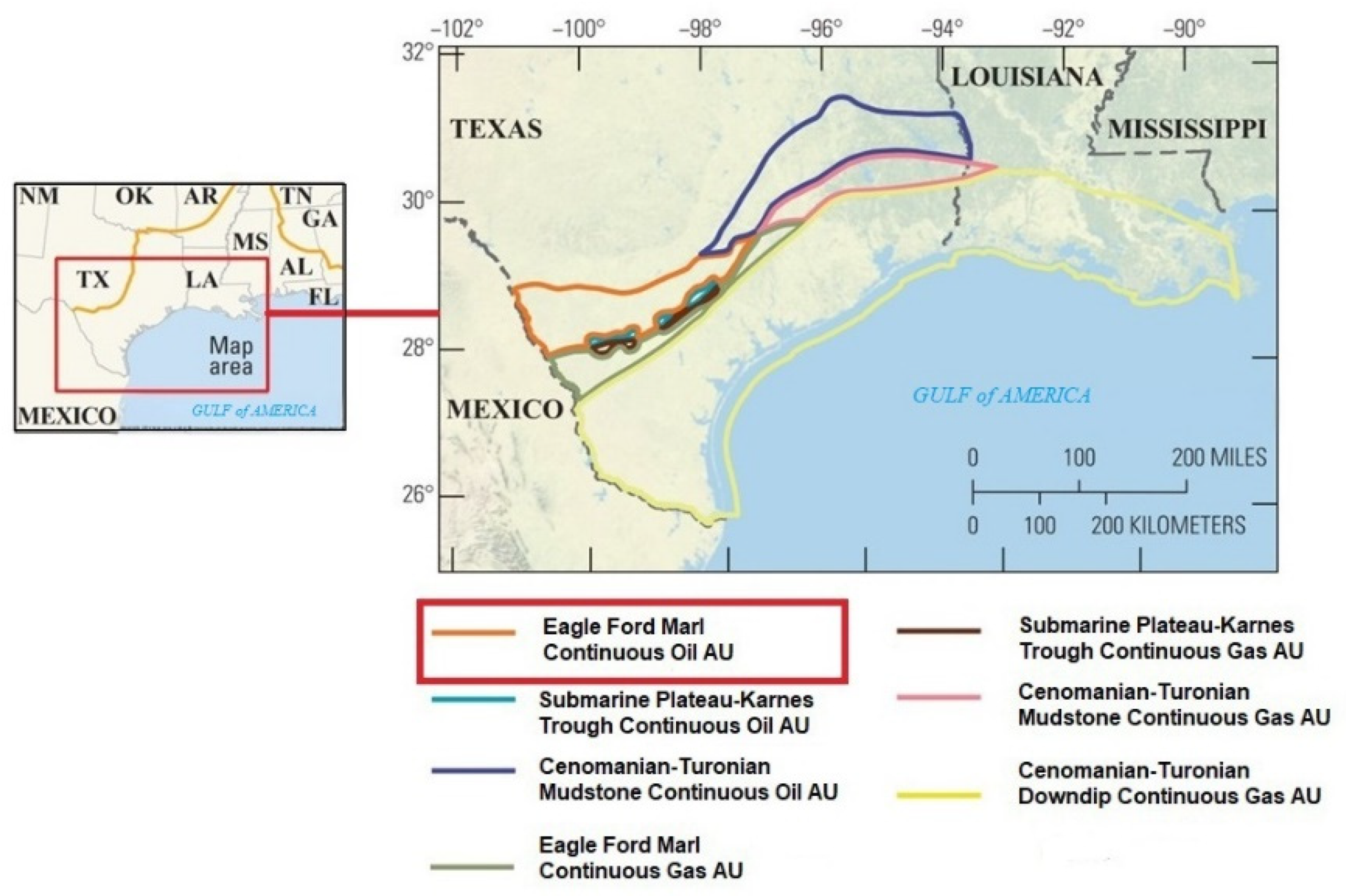
As part of its assessment of continuous (unconventional) petroleum resources in the United States, the USGS (United States Geological Survey) assessed the Eagle Ford Group and associated Cenomanian–Turonian strata with a focus on the technically recoverable resources within seven geologically defined assessment units (AUs). Whidden et al. [21] defined the AUs based on lithology, stratal thickness, thermal maturity, regional geologic features, and spatial distribution of productive fairways (Figure 2).
We used EUR data (for 11,625 wells) from the Eagle Ford Marl Continuous Oil AU. This AU contains carbonate-rich mudstones of the Eagle Ford Shale, and the term “marl” describes the lithology of rocks contained therein. The AU boundaries were determined by the United States–Mexico border, the 25% clay line separating the Eagle Ford marl (<25%) and Cenomanian–Turonian mudstone strata (>25%) to the northeast [29], and the thermal maturity window for oil (0.6–1.3 percent modeled vitrinite reflectance). Adjacent to this AU is the Submarine Plateau-Karnes Trough Continuous Oil AU, which is a zone of thicker Eagle Ford Group strata (greater than 120 feet), as mapped by Hammes et al. [25]. The 2018 USGS assessment interpreted this thicker interval to have enhanced source rock and reservoir potential [21].

3. Sources of Input Data for EUR Modeling, and Preliminary Considerations

In this study, we developed multilayer perceptron (MLP) based artificial neural networks (ANNs) to predict the EURs of wells that have produced from the upper and lower Eagle Ford Shale. This approach differs from Mehana et al. [19], who predicted Eagle Ford shale gas EURs by implementing an unsupervised-ML methodology for automatic identification of the optimal number of features (signals) present in the production data.
We used spatially collocated data for each well location from previous USGS Eagle Ford Shale assessments for well-specific EURs [21], S&P Global’s Enerdeq database for well records [30], and reservoir data geo-referenced and digitized from geostatistical maps that were published by Hammes et al. [25]. Figure 3 presents the general methodology followed in this work.

3.1. Well Specific EUR Data

The USGS continuous oil and gas resources assessment methodology focuses on geologically defined assessment units (AUs) [16]. The methodology leverages data on reservoirs that may already have significant numbers of wells (hundreds and even thousands in some cases) and well production information. Based on these data and other information, the goals of these assessments include estimation of EURs and derivation of a probability distribution to delineate the resource uncertainty within the AU.
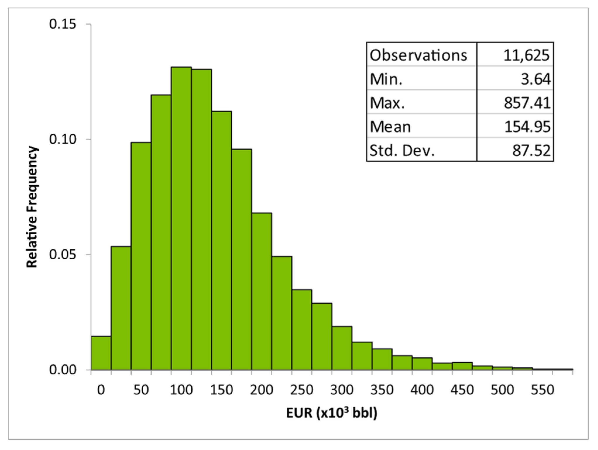
Leathers-Miller [31] documented the steps taken to estimate the EURs of the wells penetrating the Eagle Ford Marl Continuous Oil AU, which Leathers-Miller [32] also described in a data release associated with the USGS resource assessment [21]. For that assessment, monthly well production data were acquired from S&P Global’s Enerdeq database [30]. The EUR of each well was calculated using stretched exponential method in DeclinePlus software v.2 [33], which is now named ForecastTM and runs on the S&P Global Harmony interface. Valko [6] considered stretched exponential method to be more appropriate than others for use in assessment of continuous resources. The decline-based EUR for each well was estimated assuming a 60-year period of production. Wells with less than 18 months of historical production were removed from consideration due to erratic early production and potential transient flow effects. In addition, any wells with very small EURs (<2000 barrels) and wells that yielded very high EURs were screened and the production profiles were investigated for abnormalities, major discontinuities, or disruptions in production data that would raise data reliability concerns. Detailed description of the approach is given in [31]. Figure 4 shows the histogram of the decline-based EURs from the 11,625 wells that were included in the initial database constructed for this study.

3.2. Well and Reservoir Data

To populate data that might be influential on the performance of wells and (thus) could be useful for EUR prediction, we used two main data sources. We extracted well records from S&P Global’s Enerdeq database [30] via queries using the American Petroleum Institute (API) numbers corresponding to each of the 11,625 wells. The search for well records from Enerdeq yielded important data, including the type of primary fluid produced (oil or gas) and the type of well (which was almost exclusively horizontal). In addition, we extracted other potentially important well attributes from the S&P database, including IP (initial potential) test flow tubing pressure; API gravity of produced oil; oil, water, and gas production rates during IP tests; IP test gas to oil ratio (GOR); ground elevation; total drill length of each of the wells; true vertical depth (TVD); depth of the top and bottom of the perforated interval along the trajectory of the well; perforated length; total proppant and treatment fluid amounts; and depth to the top of the formation. However, not all of this information was available for every well, which resulted in a varying number of data entries for each of the wells. Since the multivariate statistical methods and ANN approach require complete datasets, we removed wells with missing values for any of these attributes from consideration. Finally, we only considered the wells producing oil as the primary fluid. Implementing these screening criteria reduced the final number of wells considered in the analysis to 3033.
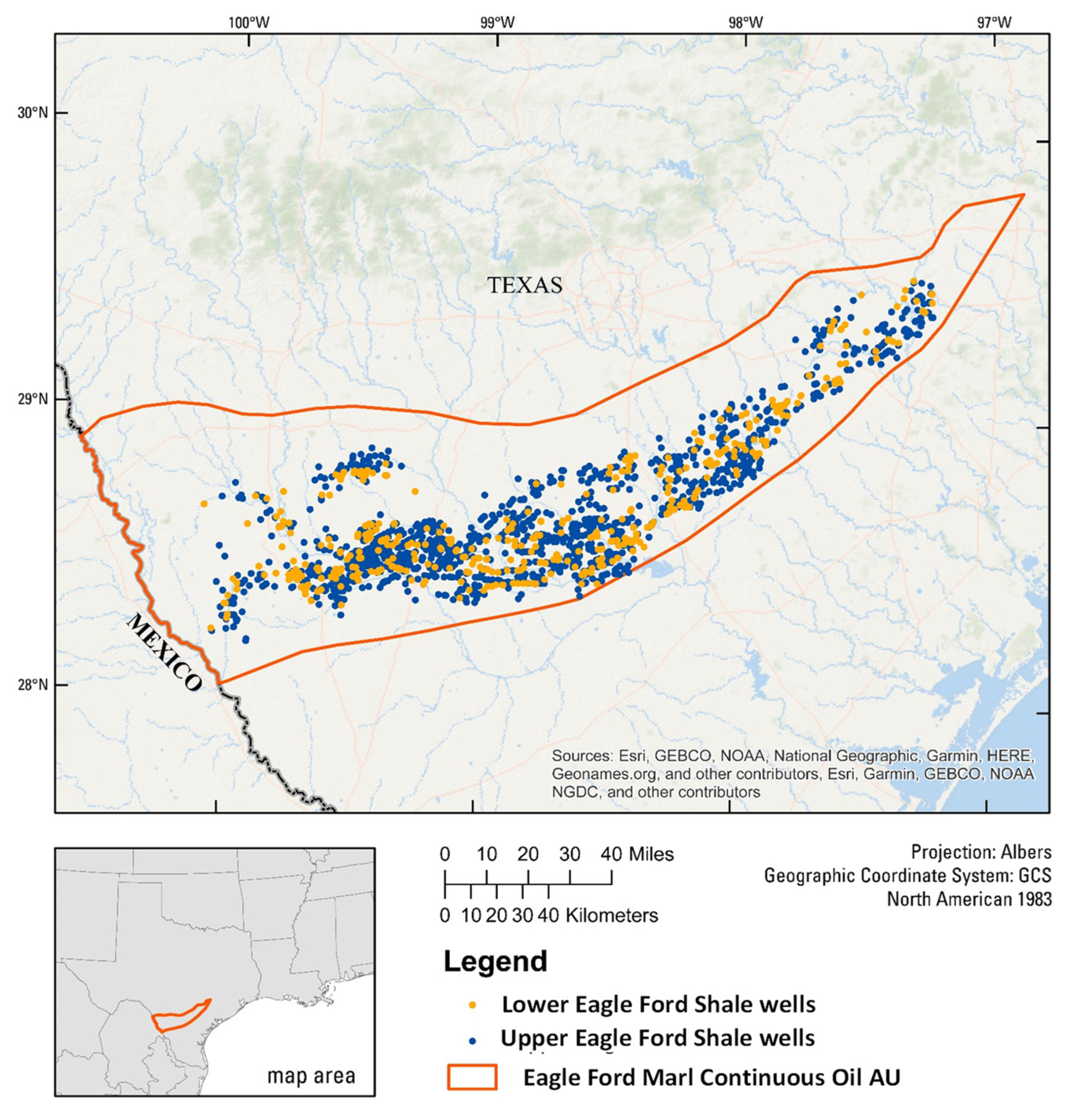
We estimated the thickness and other reservoir properties at each well site based on maps provided in [25]. We geo-referenced these maps to a base map of county outlines in ArcMap [34]. Next, we created contour lines where the values of a selected reservoir property changed in the maps and used these to create rasters using the “Topo to Raster” tool in ArcMap [34]. The rasters enabled estimation of reservoir property and thickness values at specific well locations based on latitudes and longitudes. The reservoir data included values for gross thickness, net thickness, porosity, water saturation, clay volume, and total organic carbon (TOC). Hammes et al. [25] generated and mapped these reservoir data for the lower Eagle Ford (LEF) and upper Eagle Ford (UEF) separately. Therefore, each well was allocated to its producing interval (i.e., to the LEF or UEF). First, we estimated the depth of the LEF and UEF boundaries using the thicknesses of LEF and UEF and the depth to the top of the Eagle Ford formation (extracted from Enerdeq for each well). Then, we compared the TVD of the wells with the depth of the LEF and UEF boundaries at each well site, which enabled determination of whether each well’s lateral/perforated section was in the LEF or the UEF. Finally, we merged EUR data with the digitized reservoir data and well attributes, and we partitioned the dataset according to the producing intervals (LEF or UEF) to generate two datasets populated with values of the potential explanatory variables and corresponding EUR data. The final number of wells with complete reservoir data and well attributes for the LEF and UEF were 626 and 2407, respectively. Figure 5 shows a map of the wells allocated to the UEF and LEF.
Figure 6A,B present the EUR histograms for the wells that produced from the LEF and UEF, respectively. It is important to note that our approach assumed production was solely from one interval without any contribution from the other. This meant that we assumed that the UEF did not contribute at all to LEF production despite wells that produced from the LEF having to pass through the UEF. Figure 6 shows that the distribution of EURs of the wells that produced from the LEF is similar to that for the UEF. The mean values were between 150,000 and 160,000 barrels (bbls) of oil, the minimum values were between 13,000 and 20,000 bbls, and the maximum values were between 407,000 and 420,000 bbls for the LEF and UEF, respectively, although the number of wells in the separate datasets for each interval was very different.
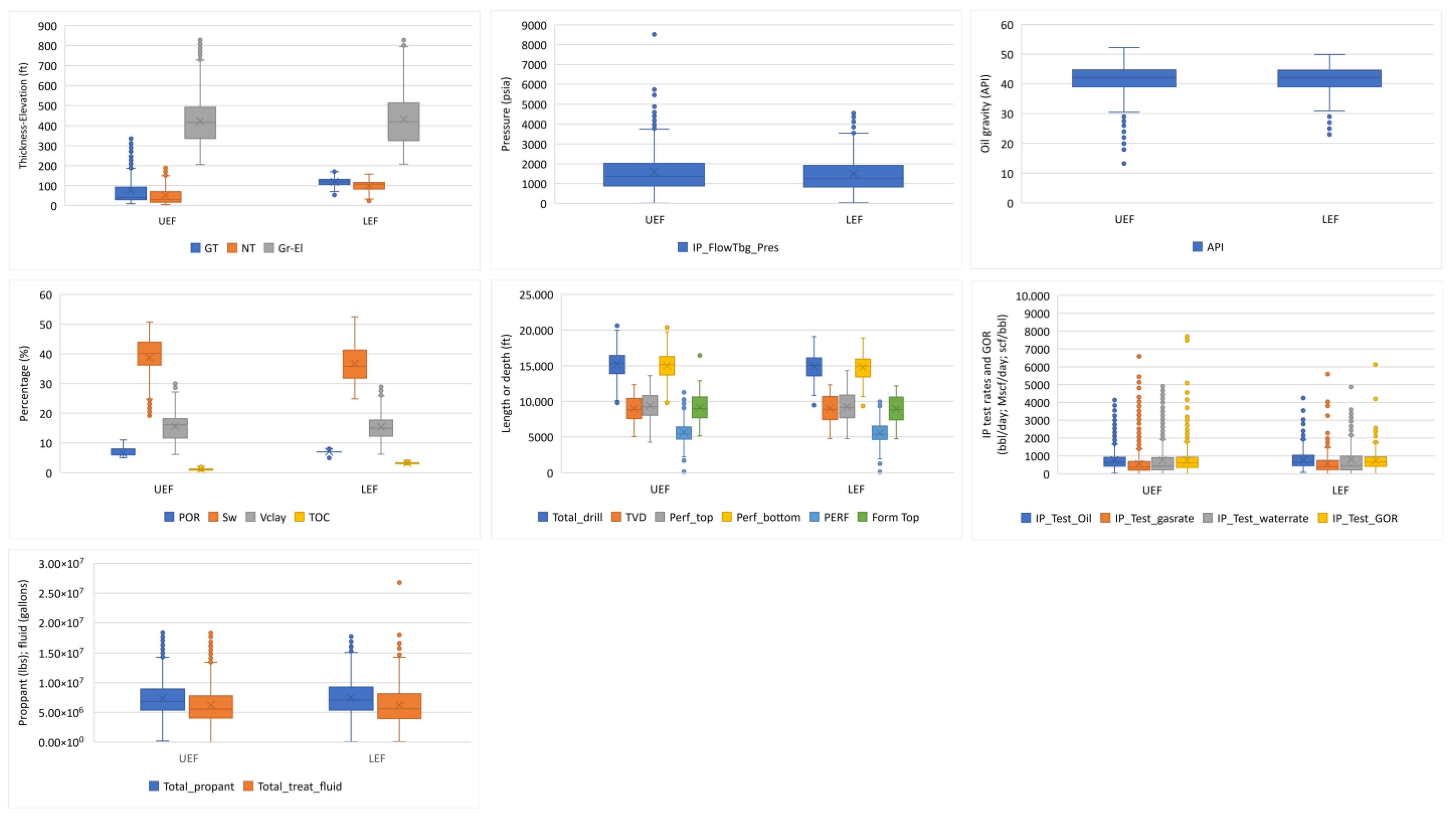
Table 1 and Table 2 display the basic statistics for well attributes and the reservoir properties at the locations of the wells that produced from the LEF and UEF, respectively. The results in Table 1 and Table 2 and Figure 7 suggest that most of the variables that reflect reservoir properties and the attributes of the wells producing from the LEF and UEF have similar values for data centrality (means and medians) and interquartile ranges (data dispersion) for both intervals. However, the ranges (maximum–minimum) and standard deviations (Table 1 and Table 2) exhibit some differences between the two intervals due to outliers shown in the box-and-whisker plots (Figure 7). Although they constituted a very small portion of the total amount of data, we did not remove these outliers, since they were not extreme outliers, and we did not have a reason to believe that these were erroneous measurements. Thus, we did not want to artificially skew the datasets or further reduce the number of observations.
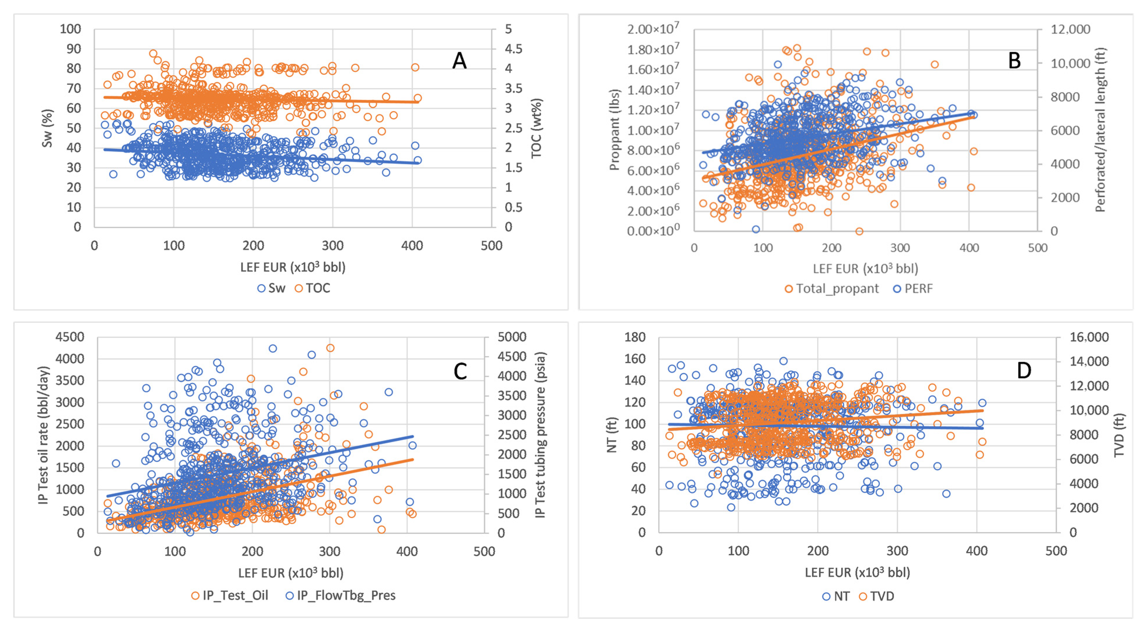
The relationships between EUR and multiple well completion and reservoir parameters can be complex. Theoretically favorable reservoir properties, such as high TOC or porosity, low water saturation (Sw), or higher reservoir thickness, could be expected to be positively correlated with EUR [25,35]. Similarly, well attributes, such as longer lateral sections or larger amounts of proppant use (indicating more intensive fracturing), could be expected to be positively correlated with EUR. In addition, greater IP test tubing pressure (as an indicator of higher reservoir pressure and thus more efficient fluid delivery for the producing life of the well) or IP test oil recovery may be expected to be positively correlated with EUR. We plotted the univariate correlations of these variables with the decline-curve EURs of wells that penetrated the LEF and present the plots in Figure 8. While these plots do not show the expected positive correlation between EUR and TOC (Figure 8A), in general, they do suggest slight negative correlation between EUR and Sw (Figure 8A), and positive correlations between EUR and IP test pressure and oil flow rate (Figure 8C), as well as between EUR and lateral wellbore length and total proppant used (Figure 8B). On the other hand, the univariate correlations between EUR and TVD appear to be slightly positively correlated, while net thickness (NT) of the LEF appear to be uncorrelated (Figure 8D). However, it should be noted that, although Figure 8 may provide some indication of the importance of these variables for predicting EUR, the explanatory power of any single variable is very limited, and the plots should not be considered as explanatory of all the variance in EUR attributable to each independent variable. Because EUR is explained by multiple variables and their interactions, the univariate correlations (or lack thereof) shown in Figure 8 may be due to other variables that are not included in one of the plots.
In general, simple regression or polynomial relationships are not sufficient to explain the relationships between EUR and the reservoir and well-completion parameters [36]. In addition, not all variables may be as important for predictive purposes as others. Thus, as in any prediction model, the selection of appropriate predictors is important in ANN modeling [37].

4. Principal Component Analysis (PCA) for Model Complexity Reduction

In this study, we used principal component analysis (PCA) for selecting the most important input variables among all the variables considered for predicting EUR of wells that produced from the LEF and UEF, respectively (Table 1 and Table 2). We performed the PCA using the XLStat statistical package [38]. Principal component analysis transforms the explanatory variables into principal components (PCs) that are orthogonal and uncorrelated to each other. To improve the interpretability of PCs, a new component matrix can be created by using Kaiser’s varimax rotation method [39], in which PC axes are rotated to a position where the sum of the variances of the loadings is a maximum [40,41,42]. Typically, the first few PCs account for most of the variance.
Table 3 presents the rotated matrix for the top five principal components, which accounted for almost 80% of cumulative variance in the data, and it shows the factor loadings of each variable within each PC for the LEF and UEF. The table also shows the separation of the variables between rotated PCs according to the well attributes or reservoir properties that they may represent. The highest factor loadings indicate that the depth to the top of the formation and the TVD of the wells are important parameters in PC1R for both the LEF and UEF, gross thickness is an important parameter in PC1R for the UEF, and net thickness of the productive interval is more important in PC2R for the LEF than for the UEF. In addition, perforated/lateral length and well-completion parameters have the highest loadings in PC2R for the UEF and in PC3R for the LEF. The IP test oil flow rate had the highest loading in PC4R for both the LEF and UEF, which suggests that the fluid delivery potential is important in both cases. Finally, intrinsic reservoir properties were important in PC5R. For the LEF, porosity had the highest loading in PC5R, whereas water saturation and TOC were weighted more heavily in PC5R for the UEF.
The relationships between most of the explanatory variables and EUR are likely to be non-linear. Therefore, the results of our PCA need to be evaluated with care. Still, the results of the PCA suggest that it is reasonable to consider the most heavily weighted input variables from each of the five PCs that captured roughly 80% of the variance in the data and further explore whether they represent properties that might be important for predicting EUR [42]. Therefore, we selected the variables with the highest loadings in each of the PCs (typed in bold in Table 3) as inputs for ANN model development.

5. Development of ANN Models for EUR Prediction—Results and Discussion

In this study, we used ANNs as a prospective predictive model for such a complex non-linear problem. However, it should be mentioned that there are other ML algorithms that can be applicable for different problems and, depending on the data, one may outperform the others. For instance, in a study predicting low salinity effect in sandstone from a set of experimental variables, Wang et al. [43] concluded that random forest (RF) outperformed support vector machine (SVM) and ANN with the lowest error, whereas Zou et al. [44] found that light gradient boosting machine (LightGBM) outperformed others tested, including RF, in predicting porosity from seismic data. Similarly, Gavriliev et al. [45] showed that distribution of predicted radon fluxes using the ANN were more realistic. Similarly, Wang et al. [18] found out that SVM outperformed neural network and Gaussian process regression model in predicting EUR of CBM wells. These studies suggest that there is no one-fits-all model and the model performance can be highly dependent on the data. Nevertheless, due to its proven performance in complex non-linear problems and that testing of different algorithms was not the main focus of this work, we proceeded only with the ANN in this study.
An ANN governs computational input–output information flow through the connections of simple processing elements, called neurons, which are networked by using different topologies in the form of input–output and hidden layers [46,47,48]. Multilayer perceptron (MLP) is one of the most widely used topologies for complex problems, where transfer functions propagate the information between different layers. Although recently ANNs included more advanced features for different problems, e.g., complex signal prediction using convolutional neural networks with an attention mechanism [49], in this study, we used a more classical approach with hyperbolic tangent as the transfer function, which can improve the performance of a neural network for predicting parameters that are highly non-linear functions of many variables (such as EUR). We used momentum as the learning algorithm and optimized it during hyper-parameter search process [50].
The theory, functional elements, properties, and important considerations for MLP development and application are described in many analyses in the literature [51,52,53] and are not repeated in detail here. The following section presents the error results of the hyper-parameter optimization search that led to the final specifications of the ANN models and informed results of this study.

5.1. Preliminary Models for Hyper-Parameter Search

Since there were two productive intervals (LEF and UEF) in the Eagle Ford Marl Continuous Oil AU, we constructed two separate ANN models. This yielded a model with two hidden layers for the LEF and a model with three hidden layers for the UEF. The input–output patterns, which were determined in part by the results of the PCA in this study, may have impacted the number of hidden layers in these ANN models [53]. For modeling the LEF, 80% of the final LEF dataset (626) was allocated for training and 10% each for cross-validation and testing. In the UEF modeling, 90% of the UEF dataset (2407) was allocated for training, and 5% (about 120 observations) each for cross-validation and testing. The differences in the allocations of observations in the two datasets was due to the difference in the number of total observations in each dataset (626 for the LEF and 2407 for the UEF) and the need to have enough data for adequate training, cross-validation, and meaningful testing with predictive results covering the range of expected values. In this study, we used 501 observations for training and 63 each for cross-validation and testing of the LEF model, whereas the more extensive UEF dataset allowed us to use 2166 observations for training and 120 each for cross-validation and testing.
We used a heuristic approach, meaning adjusting different hyper-parameters, for their optimization. The strategy began with determining the layer structures (two and three hidden layers for LEF and UEF, respectively) for modeling the productive intervals. Within the parameters that can be adjusted, the number of neurons in each of the hidden layers and the momentum factors were evaluated as most important for learning and predictive capabilities of the models. Therefore, optimization included a varying number of neurons in the hidden layers and the momentum factors to evaluate training errors for deciding the best performing networks.
Table 4 presents the mean squared errors obtained using different hidden-layer (HL) neurons and momentum factors for the LEF and UEF models. The HL neurons and momentum factors that resulted in the minimum MSE for each case in Table 4 were selected as the combination of the parameters of the final models. Following this approach, we constructed the LEF model with 25 and 21 neurons in the first and second hidden layers, respectively, and we selected 0.6 as the factor of the momentum learning. Similarly, we constructed the UEF model using 44, 38, and 26 neurons in the hidden layers 1, 2, and 3, respectively, and we again selected a momentum factor of 0.6 for the UEF model. Also, as part of the heuristic approach, we tested with the number of training epochs for the model to learn the patterns with a minimal risk of memorizing them. We determined that 5000 training epochs for the LEF and 10,000 epochs for the UEF were sufficient for training of the models.

5.2. Training, Cross-Validation and Testing of Final Models: Results of EUR Prediction

This section describes the results of the final EUR prediction models for the LEF and UEF. In terms of just comparing the mean squared errors for training and cross-validation, the LEF model achieved MSEs of 0.00959 and 0.01904, respectively, and the UEF model performed slightly worse than the LEF model, with a 0.01214 MSE for training and 0.01904 for the cross-validation MSE.
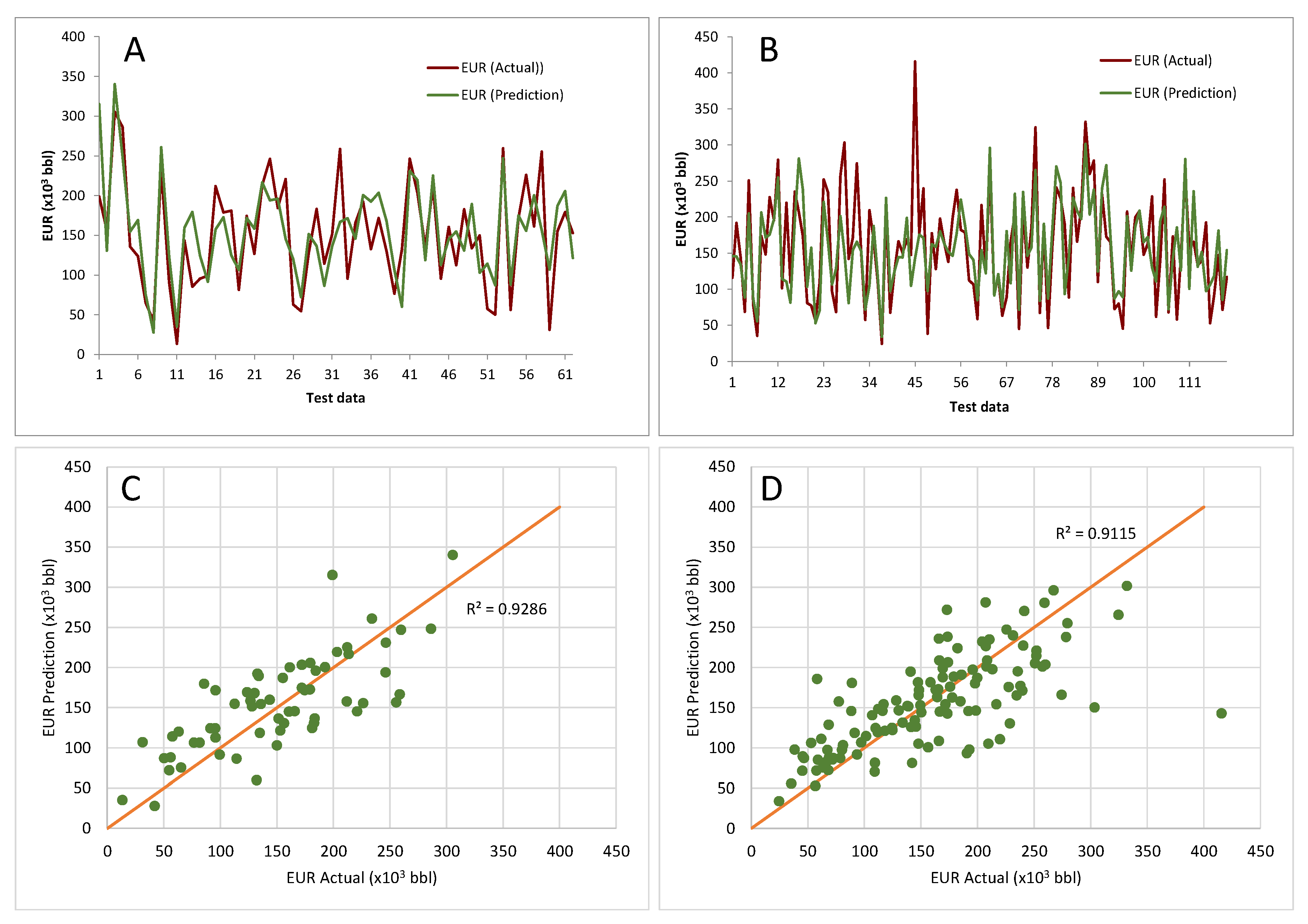
Figure 9 shows comparisons of the EURs based on DCA with the ANN predictions for the LEF (Figure 9A,C) and UEF (Figure 9B,D) models using test data. In general, Figure 9A,B show that the predictions of the ANN models align well with the DCA-based EURs, despite some notable discrepancies at some of the data points used as testing data. The performance measures of the ANN models given in Table 5 support this interpretation of the plots in Figure 9. The mean absolute errors are around 37 × 103 bbl for both models, and the maximum errors vary depending on the departure of the predictions from the actual (DCA-based) data. The maximum error is greater in the UEF model (272.9 × 10³ bbl) than in the LEF model (116.2 × 10³ bbl), but this is owing to only one data point that the ANN model did not predict as well with the given input data or the network parameters. Regression plots considering all data points (Figure 9C,D) show a good correlation between actual (decline curve) and predicted values with R2 > 0.9 for both models.
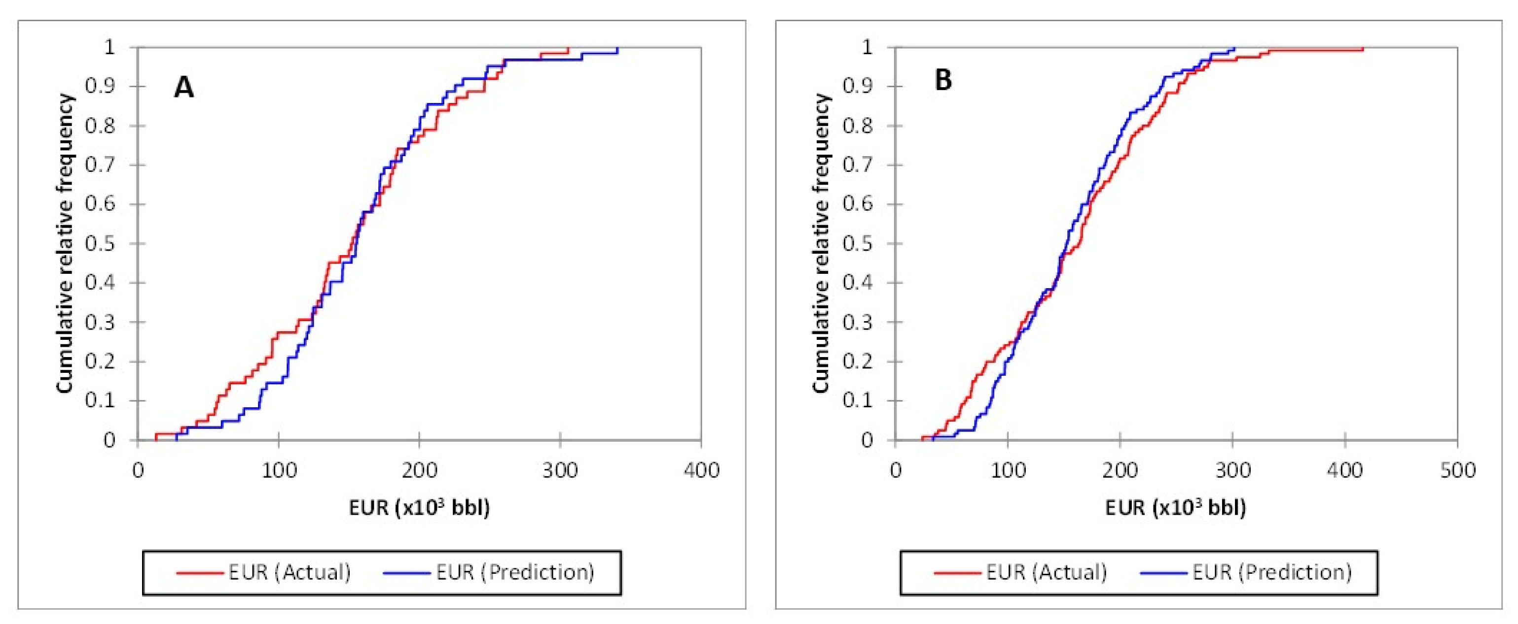
Although Figure 9 shows that there is a reasonably good correlation between actual and ANN-predicted values for both the LEF and UEF, there is notable scatter around the 1:1 line in both cases. This could imply that the decline-curve values and the ANN-predicted values may follow different cumulative distribution functions. To test the null hypothesis that these two sets of EUR values could be sampled from the same distribution, we used the two-sample Kolmogorov–Smirnov (KS) test [54]. The two-sample KS test is a nonparametric test of the equality of one-dimensional probability distributions. It is one of the most useful and general nonparametric methods for testing whether two samples could be considered as drawn from significantly different populations, because it is sensitive to differences in the shape of the cumulative distribution functions. The test compares the KS statistic (d) across the two distributions with a probability (p-value) for a given significance level. The d- and p-values are the parameters of the KS test that determine whether the null hypothesis can or cannot be rejected. The null hypothesis is rejected if the d-value is greater than the critical p-value obtained for a chosen significance level and if the critical p-value is less than that corresponding to the chosen significance level. If the KS test indicates that the null hypothesis cannot be rejected, the p-value indicates the risk of rejecting the hypothesis. We assumed a 5% significance level to compare the actual and ANN-predicted EUR values in the test dataset. Figure 10A,B present the cumulative distribution functions of the actual and ANN-predicted EUR values for the test data for the LEF and UEF intervals, respectively. In Figure 10, the distributions of the actual data and the predictions by the LEF (A) and UEF (B) models suggest that they are generally close to each other.
Table 6 gives the basic statistics and KS statistics for the actual and ANN-predicted values of EUR for both the LEF and UEF. The basic statistics of centrality and spread of the data support the claim that the distribution of the actual EURs follow a distribution that is similar to that of the ANN-predicted EUR values. The KS tests for both models indicated that the d-values were greater than the p-values, and therefore the null hypothesis that the samples follow the same distribution could not be rejected. The risk of rejecting the null hypothesis was 69% and 31% for the LEF and UEF, respectively. In addition to the errors and the correlations between actual and ANN-predicted values, the results in Figure 10 and Table 6 may also suggest that the models predicted EURs reasonably well.
Finally, we tested the models for sensitivities about the mean values of the input parameters. In these tests, the value of the parameter being tested was varied one standard deviation about its mean value, while that of all other parameters were held fixed at their mean values. Figure 11 shows that the EUR predictions for the LEF model were most sensitive to changes in porosity, net thickness of the interval, clay volume, and the API gravity of the oil. The EUR predictions for the UEF model were most sensitive to changes in the TOC and water saturation. In the case of the LEF, which is the main source of Eagle Ford production [35], we found that changes in porosity and net thickness had the greatest impact on predictions of EUR. Hou et al. [1] indicated that these parameters were highly correlated with reservoir capacity and hydrocarbons in-place in the Eagle Ford Shale. In other applications, Ver Hoeve et al. [55] demonstrated that they could also be useful for identifying sweet spots in shale reservoirs. Hammes et al. [25] found that porosity exhibited a strong correlation with productivity in most of the Eagle Ford shale play, except in Dewitt, Karnes, and Webb Counties, but the lower correlations there could have been owing to other factors (such as low TOC). In addition, porosity and clay volume may impact permeability, which along with API gravity of the oil impacts deliverability. Therefore, the variables we found to be most important for production and EUR of the LEF in this study could be owing to them being mostly related to reservoir capacity and deliverability.
For the UEF, we found the changes in TOC and water saturation, and to a lesser degree gross thickness and oil gravity, to impact predicted EURs more than changes in other variables. Water saturation can impact both reservoir capacity and oil deliverability, while TOC represents the amount of organic matter present, which makes it important for hydrocarbon quantification and quality measurement. In addition, TOC may impact reservoir wettability and fluid adsorption [56,57], which could ultimately impact fluid mobility and deliverability. Finally, a possible relationship of TOC with reservoir geomechanics could be important for reservoir stimulation, particularly hydraulic fracturing, and it may impact fracture conductivity, deliverability, and EUR via this relationship. Several studies [58,59] have reported that the elastic modulus of shale is negatively correlated with the presence and quantity of soft materials (such as TOC), and they have observed generally ductile behavior in these cases. Although it is not the only factor, higher brittleness typically results in better fracturing effectiveness [60,61], which may also help explain the sensitivity of EUR to variations in TOC in our model of the UEF.
The results of the sensitivity tests suggest well attributes and reservoir properties that may have the greatest impact on the EUR of the wells producing from two different productive intervals of the Eagle Ford Shale. This suggests that consideration of these parameters could be important in locating productive areas for future drilling and predicting the EUR either separately for these intervals or for the entire Eagle Ford Marl Continuous Oil AU.

6. Summary and Conclusions

This study combined well-specific production and completion data and reservoir properties of the lower and upper Eagle Ford Shale with decline curve analysis (DCA)-based estimated ultimate recoveries (EURs) to develop, train, and test multilayer perceptron (MLP)-based artificial neural network (ANN) models. Below are the main conclusions:
  • The preliminary analysis based on univariate correlations indicated that none of the variables included in the dataset for this study exhibited a strong univariate correlation with the DCA-based EURs, which suggested that EUR is a complex function of multiple variables. To select the variables that accounted for most of the variation in the dataset, we performed a principal component analysis (PCA).
  • The results of the PCA suggested that the TVD of the wells, formation thickness, perforated/lateral length, and completion parameters, as well as some variables related to fluid delivery potential and intrinsic reservoir properties (porosity, water saturation, and TOC) accounted for most of the variation for both the lower Eagle Ford (LEF) and upper Eagle Ford (UEF). Therefore, we used these variables to construct the ANN models.
  • For both the LEF and UEF, training and testing results of optimized ANN models suggested that the approach could be promising for predicting EURs with acceptable accuracy. Indeed, besides the error results, the two-sample Kolmogorov–Smirnov (KS) tests conducted to compare actual (DCA-based) and ANN-predicted EUR values suggested that both sets of EUR values could have been drawn from the same distribution. This suggests that the EURs predicted by the ANN models were reasonable estimates, and that the ANN approach could be useful in corroborating estimates of the EUR based on more traditional approaches.
  • In addition, this approach could provide preliminary estimates of EURs for plays with extensive geological data, but with no wells or very little production history. However, the extent to which applying our approach to a hypothetical play or other plays with almost no productive history could provide reasonable predictions of the EUR would likely depend on how close of an analog the play is to the assessment units (AUs) used to source existing (DCA-based) EUR data. We also tested the sensitivities of the ANN-predictions of EUR to changes around the mean values of the input variables. The differences in the EUR predictions for the LEF were most sensitive to changes in porosity, net thickness of the interval, clay volume and the API gravity of the oil. The differences in the EUR predictions for the UEF were most sensitive to changes in the total organic carbon (TOC) and water saturation.
  • The results of this sensitivity analysis indicated the importance of considering these parameters in predicting EURs for these intervals. Since the model predictions for the LEF were most sensitive to changes in a different set of parameters than that for the UEF, this could suggest that EUR predictions using this approach could vary based on the selected production interval, even within the same formation or AU. It could also suggest that using either the LEF or the UEF individually as an analog could be more appropriate for applying this method to predict the EUR of a new AU. In future work, integration of other important reservoir properties (such as permeability) or geomechanical variables (e.g., Young’s modulus) may improve the predictive capability of the ANN models developed here, but data on these additional parameters for the Eagle Ford Shale were not available to the extent necessary to consider them in this study. In addition, although we have shown that the MLP-ANN can be a useful approach, other machine learning and fuzzy-inference methods exist and could be tested for their predictive performance relative to each other to select the “best” modeling approach. Finally, this study focused on integrating data from different sources to develop MLP-based ANN models for a specific application to the Eagle Ford Shale continuous oil marl AU, and it could be useful to apply the methods developed here to other AUs.

Author Contributions

Conceptualization, C.Ö.K. and S.T.A.; Methodology, C.Ö.K.; Validation, C.Ö.K. and S.T.A.; Formal Analysis, C.Ö.K.; Investigation, C.Ö.K. and S.T.A.; Resources, C.Ö.K., S.T.A. and S.M.C.; Data Curation, C.Ö.K. and S.M.C.; Writing—Original Draft Preparation, C.Ö.K.; Writing—Review and Editing, C.Ö.K., S.T.A. and S.M.C.; Visualization, C.Ö.K., S.M.C. All authors have read and agreed to the published version of the manuscript.

Funding

This research received no external funding.

Data Availability Statement

The authors do not have permission to share the dataset. The sources are cited and the original contributions presented in this study are included in the article. Further inquiries can be directed to the corresponding author.

Acknowledgments

The authors would like to thank Heidi M. Leathers-Miller of the U.S. Geological Survey (USGS) for providing DCA-based EUR data for this study. The authors would also like to thank William H. Craddock (USGS) for reviewing an earlier version of this paper and his helpful comments. Acknowledgements are also extended to the editor and the journal reviewers for their positive feedback that improved the final manuscript. Any use of trade, firm, or product names is for descriptive purposes only and does not imply endorsement by the U.S. Government.

Conflicts of Interest

The authors declare that the research was conducted in the absence of any commercial or financial relationships that could be construed as a potential conflict of interest.

References

  1. Hou, L.; Yu, Z.; Luo, X.; Lin, S.; Zhao, Z.; Yang, Z.; Wu, S.; Cui, J.; Zhang, L. Key geological factors controlling the estimated ultimate recovery of shale oil and gas: A case study of the Eagle Ford Shale, Gulf Coast Basin, USA. Pet. Explor. Dev. 2021, 48, 762–774. [Google Scholar] [CrossRef]
  2. Wang, K.; Li, H.; Wang, J.; Jiang, B.; Bu, C.; Zhang, Q.; Luo, W. Predicting production and estimated ultimate recoveries for shale gas wells: A new methodology approach. Appl. Energy 2017, 206, 1416–1431. [Google Scholar] [CrossRef]
  3. Xi, Z.; Morgan, M. Combining decline-curve analysis and geostatistics to forecast gas production in the Marcellus Shale. SPE Reserv. Eval. Eng. 2019, 22, 1562–1574. [Google Scholar] [CrossRef]
  4. Weijermars, R.; Tugan, M.F.; Khanal, A. Production rates and EUR forecasts for interfering parent-parent wells and parent-child wells: Fast analytical solutions and validation with numerical reservoir simulators. J. Pet. Sci. Eng. 2020, 190, 107032. [Google Scholar] [CrossRef]
  5. Li, B.; Billiter, T.C.; Tokar, T. Rescaling method for improved machine-learning decline curve analysis for unconventional reservoirs. SPE J. 2021, 26, 1759–1772. [Google Scholar] [CrossRef]
  6. Valko, P.P. Assigning value to stimulation in the Barnett Shale: A simultaneous analysis of 7000 plus production histories and well completion records. In Proceedings of the SPE Hydraulic Fracturing Technology Conference, The Woodlands, TX, USA, 19–21 January 2009. Paper SPE-119369-MS. [Google Scholar] [CrossRef]
  7. Duong, A.N. An Unconventional rate decline approach for tight and fracture dominated gas wells. In Proceedings of the Canadian Unconventional Resources and International Petroleum Conference, Calgary, AB, Canada, 19–21 October 2010. Paper SPE-137748-MS. [Google Scholar] [CrossRef]
  8. Clarkson, C.R. Production data analysis of unconventional gas wells: Review of theory and best practices. Int. J. Coal Geol. 2013, 109, 101–146. [Google Scholar] [CrossRef]
  9. Mehana, M.; Callard, J. Reserve estimation with unified production analysis. In Proceedings of the 6th Unconventional Resources Technology Conference, Houston, TX, USA, 23–25 July 2018; URTEC-2901909-MS. pp. 691–696. [Google Scholar] [CrossRef]
  10. Korde, A.; Goddard, S.D.; Obadare, O.A. Probabilistic decline curve analysis in the Permian Basin using Bayesian and approximate Bayesian inference. SPE Reserv. Eval. Eng. 2021, 24, 536–551. [Google Scholar] [CrossRef]
  11. Shin, H.-J.; Lim, J.-S.; Shin, S.-H. Estimated ultimate recovery prediction using oil and gas production decline curve analysis and cash flow analysis for resource play. Geosyst. Eng. 2014, 17, 78–87. [Google Scholar] [CrossRef]
  12. Sharma, A.; Lee, W.J. Improved workflow for EUR prediction in unconventional reservoirs. In Proceedings of the 4th Unconventional Resources Technology Conference, San Antonio, TX, USA, 1–3 August 2016; URTEC-2444280-MS. pp. 961–978. [Google Scholar] [CrossRef]
  13. Male, F. Assessing impact of uncertainties in decline curve analysis through hindcasting. J. Pet. Sci. Eng. 2019, 172, 340–348. [Google Scholar] [CrossRef]
  14. Mehana, M.; Callard, J.; Kang, Q.; Viswanathan, H. Monte Carlo simulation and production analysis for ultimate recovery estimation of shale wells. J. Nat. Gas Sci. Eng. 2020, 83, 103584. [Google Scholar] [CrossRef]
  15. Male, F.; Duncan, I.J. The paradox of increasing initial oil production but faster decline rates in fracking the Bakken Shale: Implications for long term productivity of tight oil plays. J. Pet. Sci. Eng. 2022, 208, 109406. [Google Scholar] [CrossRef]
  16. Charpentier, R.R.; Cook, T.A. Improved USGS Methodology for Assessing Continuous Petroleum Resources, Version 2.0. U.S. Geological Survey Data Series 547 and Program. U.S. Geol. Surv. Data Ser. 547, U.S. Department of the Interior, U.S. Geological Survey, 2010. Available online: https://pubs.usgs.gov/publication/ds547 (accessed on 18 August 2025).
  17. Attanasi, E.D.; Freeman, P.A. Economic Analysis of the 2010 U.S. Geological Survey Assessment of Undiscovered Oil and Gas in the National Petroleum Reserve in Alaska; U.S. Geological Survey Open-File Report 2011-1103; U.S. Department of the Interior, U.S. Geological Survey; 2011. Available online: https://pubs.usgs.gov/publication/ofr20111103 (accessed on 18 August 2025).
  18. Wang, F.; Wu, M.; Wang, Y.; Sun, W.; Chen, G.; Feng, Y.; Shi, X.; Zhao, Z.; Liu, Y.; Lu, S. Prediction of Influencing Factors on Estimated Ultimate Recovery of Deep Coalbed Methane: A Case Study of the Daning–Jixian Block. Processes 2025, 13, 31. [Google Scholar] [CrossRef]
  19. Mehana, M.; Guiltinan, E.; Vesselinov, V.; Middleton, R.; Hyman, J.D.; Kang, Q.; Viswanathan, H. Machine-learning predictions of the shale wells’ performance. J. Nat. Gas Sci. Eng. 2021, 88, 103819. [Google Scholar] [CrossRef]
  20. Liu, Y.-Y.; Ma, X.-H.; Zhang, X.-W.; Wei, G.; Kang, L.-X.; Yu, R.-Z.; Sun, Y.-P. A deep-learning-based prediction method of the estimated ultimate recovery (EUR) of shale gas wells. Pet. Sci. 2021, 18, 1450–1464. [Google Scholar] [CrossRef]
  21. Whidden, K.J.; Pitman, J.K.; Pearson, O.N.; Paxton, S.T.; Kinney, S.A.; Gianoutsos, N.J.; Schenk, C.J.; Leathers-Miller, H.M.; Birdwell, J.E.; Brownfield, M.E.; et al. Assessment of Undiscovered Oil and Gas Resources in the Eagle Ford Group and Associated Cenomanian–Turonian Strata, U.S. Gulf Coast, Texas, 2018; U.S. Geological Survey Fact Sheet 2018–3033; U.S. Department of the Interior, U.S. Geological Survey; 2018. Available online: https://pubs.usgs.gov/publication/fs20183033 (accessed on 18 August 2025).
  22. Dubiel, R.F.; Pearson, O.N.; Pitman, J.K.; Pearson, K.M.; Kinney, S.A. Geology and sequence stratigraphy of undiscovered oil and gas resources in conventional and continuous petroleum systems in the Upper Cretaceous Eagle Ford Group and related strata, U.S. Gulf Coast region. Gulf Coast Assoc. Geol. Soc. Trans. 2012, 62, 57–72. [Google Scholar]
  23. Dawson, W.C. Shale microfacies: Eagle Ford Group (Cenomanian-Turonian) North-Central Texas outcrops and subsurface equivalents. Trans.—Gulf Coast Assoc. Geol. Soc. 2000, 50, 607–622. [Google Scholar]
  24. Denne, R.A.; Breyer, J.A. Regional Depositional Episodes of the Cenomanian–Turonian Eagle Ford and Woodbine Groups of Texas; Breyer, J.A., Ed.; The Eagle Ford Shale—A renaissance in U.S. oil production (AAPG Memoir 110); American Association of Petroleum Geologists: Tulsa, OK, USA, 2016; pp. 87–133. [Google Scholar]
  25. Hammes, U.; Eastwood, R.; McDaid, G.; Vankov, E.; Gherabati, S.A.; Smye, K.; Shultz, J.; Potter, E.; Ikonnikova, S.; Tinker, S. Regional assessment of the Eagle Ford Group of south Texas, USA—Insights from lithology, pore volume, water saturation, organic richness, and productivity correlations. Interpretation 2016, 4, SC125–SC150. [Google Scholar] [CrossRef]
  26. Donovan, A.D.; Staerker, T.S.; Pramudito, A.; Gardner, R.D.; Pope, M.C.; Corbett, M.J.; Lowery, C.M.; Romero, A.M. A 3-D outcrop perspective of an unconventional carbonate mudstone reservoir. In Proceedings of the Unconventional Resources Technology Conference, Denver, CO, USA, 12–14 August 2013. Paper URTEC-1580954-MS. [Google Scholar] [CrossRef]
  27. Donovan, A.D.; Staerker, T.S.; Pramudito, A.; Li, W.; Corbett, M.J.; Lowery, C.M.; Romero, A.M.; Gardner, A.D. The Eagle Ford outcrops of East Texas: Understanding heterogeneities within unconventional mudstone reservoirs. GCAGS J. 2012, 1, 162–185. [Google Scholar]
  28. Phelps, R.M.; Kerans, C.; Da-Gama, R.O.B.P.; Jeremiah, J.; Hull, D.; Loucks, R.G. Response and recovery of the Comanche carbonate platform surrounding multiple Cretaceous oceanic anoxic events, northern Gulf of Mexico. Cretac. Res. 2015, 54, 117–144. [Google Scholar] [CrossRef]
  29. Donovan, A.D.; Evenick, J.; Banfield, L.; McInnis, N.; Hill, W. An organofacies-based mudstone classification for unconventional tight rock and source rock plays. In Proceedings of the 5th Unconventional Resources Technology Conference, Austin, TX, USA, 24–26 July 2017; URTEC-2715154-MS. pp. 3683–3697. [Google Scholar] [CrossRef]
  30. S&P Global Commodity Insights. Enerdeq U.S. Well History and Production. Database Available from S&P Global Commodity Insights. 2023. Available online: https://spglobal.com/commodityinsights (accessed on 5 February 2023).
  31. Leathers-Miller, H.M. Steps Taken for Calculating Estimated Ultimate Recoveries of Wells in the Eagle Ford Group and Associated Cenomanian–Turonian Strata, U.S. Gulf Coast, Texas, 2018; U.S. Geological Survey Scientific Investigations Report 2020–5077; U.S. Department of the Interior, U.S. Geological Survey; 2020. Available online: https://pubs.usgs.gov/publication/sir20205077 (accessed on 18 August 2025).
  32. Leathers-Miller, H.M. Estimated Ultimate Recoveries of Oil Wells in the Eagle Ford Group and Associated Cenomanian–Turonian Strata, U.S. Gulf Coast 2024, Texas, 2018; U.S. Department of the Interior, U.S. Geological Survey; 2024. Available online: https://www.sciencebase.gov/catalog/item/64f9e883d34ed30c2054ae36 (accessed on 18 August 2025).
  33. IHS Markit DeclinePlus Software, version 2; IHS Markit: London, UK, 2015. Information on Current Version (Forecast) Under Harmony Enterprise Environment. Available online: https://www.ihsenergy.ca/support/documentation_ca/Harmony_Enterprise/latest/content/print_pdf_output/harmony_enterprise_help.pdf (accessed on 18 August 2025).
  34. ESRI. ArcGIS Desktop: Release, version 10.8.2; Environmental Systems Research Institute: Redlands, CA, USA, 2021.
  35. Gherabati, S.A.; Hammes, U.; Male, F.; Browning, J. Assessment of hydrocarbon in place and recovery factors in the Eagle Ford Shale play. SPE Reserv. Eval. Eng. 2018, 21, 291–306. [Google Scholar] [CrossRef]
  36. Liang, Y.; Liao, L.; Guo, Y. A Big Data Study: Correlations between EUR and petrophysics/engineering/production parameters in shale formations by data regression and interpolation analysis. In Proceedings of the Paper SPE-194381-MS Presented at the SPE Hydraulic Fracturing Technology Conference, The Woodlands, TX, USA, 5–7 February 2019. [Google Scholar] [CrossRef]
  37. Faraway, J.; Chatfield, C. Time series forecasting with neural networks: A comparative study using airline data. Appl. Stat. 1998, 47, 231–250. [Google Scholar] [CrossRef]
  38. Addinsoft Xlstat-Pro: User’s Manual. New York, NY, USA, 2007. Current Version. Available online: https://www.xlstat.com/ (accessed on 18 August 2025).
  39. Kaiser, H.F. The varimax criterion for analytic rotation in factor analysis. Psychometrika 1958, 23, 187–200. [Google Scholar] [CrossRef]
  40. Grima, M.A.; Bruines, P.A.; Verhoef, P.N.W. Modeling tunnel boring machine performance by neuron-fuzzy methods. Tunn. Undergr. Space Technol. 2000, 15, 259–269. [Google Scholar] [CrossRef]
  41. Davis, J.C. Statistics and Data Analysis in Geology, 2nd ed.; Wiley and Sons: New York, YN, USA, 1986. [Google Scholar]
  42. Karacan, C.Ö. Modeling and prediction of ventilation methane emissions of U.S. longwall mines using supervised artificial neural networks. Int. J. Coal Geol. 2008, 73, 371–387. [Google Scholar] [CrossRef]
  43. Wang, L.; Tian, L.; Yao, B.; Yu, X. Machine learning analyses of low salinity effect in sandstone porous media. J. Porous Media 2020, 23, 731–740. [Google Scholar] [CrossRef]
  44. Zou, C.; Zhao, L.; Fei, H.; Wang, Y.; Chen, Y.; Geng, J. A comparison of machine learning methods to predict porosity in carbonate reservoirs from seismic-derived elastic properties. Geophysics 2023, 88, B101–B120. [Google Scholar] [CrossRef]
  45. Gavriliev, S.; Petrova, T.; Miklyaev, P.; Karfidova, E. Predicting radon flux density from soil surface using machine learning and GIS data. Sci. Total Environ. 2023, 903, 166348. [Google Scholar] [CrossRef]
  46. Eberhart, R.C.; Dobbins, R.W. Neural Network PC Tools: A Practical Guide; Academic Press Inc.: San Diego, CA, USA, 1990. [Google Scholar]
  47. Flood, I.; Kartam, N. Neural networks in civil engineering I: Principles and understanding. J. Comput. Civ. Eng. 1994, 8, 131–148. [Google Scholar] [CrossRef]
  48. Maier, H.R.; Dandy, G.C. Neural networks for the prediction and forecasting of water resources variables: A review of modeling issues and applications. Environ. Model. Softw. 2000, 15, 101–124. [Google Scholar] [CrossRef]
  49. Wei, C.; Quan, Z.; Qian, Z.; Pang, H.; Su, Y.; Wang, L. An attention mechanism augmented CNN-GRU method integrating optimized variational mode decomposition and frequency feature classification for complex signal forecasting. Expert Syst. Appl. 2025, 269, 126464. [Google Scholar] [CrossRef]
  50. Hassoun, M.H. Fundamentals of Artificial Neural Networks; MIT Press: Cambridge, MA, USA, 1995. [Google Scholar]
  51. Rogerson, J. Recent Progress in Artificial Neural Networks; Clanrye International: New York, NY, USA, 2019. [Google Scholar]
  52. Khan, S. Backpropagation-Based Multilayer Perceptron Neural Networks. MATLAB Central File Exchange. Available online: https://www.mathworks.com/matlabcentral/fileexchange/66477-backpropagation-based-multi-layer-perceptron-neuralnetworks. (accessed on 12 November 2020).
  53. Karacan, C.Ö. Multilayer Perceptrons. In Encyclopedia of Mathematical Geosciences. Encyclopedia of Earth Sciences Series, 1st ed.; Sagar, B.S.D., Cheng, Q., McKinley, J., Agterberg, F., Eds.; Springer: Cham, Switzerland, 2023; pp. 951–954. [Google Scholar] [CrossRef]
  54. Schröer, G.; Trenkler, D. Exact and randomization distributions of Kolmogorov-Smirnov tests two or three samples. Comput. Stat. Data Anal. 1995, 20, 185–202. [Google Scholar] [CrossRef]
  55. Ver Hoeve, M.; Meyer, C.; Preusser, J.; Makowitz, A. Basinwide Delineation of Gas-Shale “Sweet Spots” Using Density and Neutron Logs: Implications for Qualitative and Quantitative Assessment of Gas-Shale Resources; Chatellier, J., Jarvie, D., Eds.; Critical Assessment of Shale Resource Plays (AAPG Memoir 103); American Association of Petroleum Geologists: Tulsa, OK, USA, 2013; Chapter 9; pp. 151–165. [Google Scholar]
  56. Pan, B.; Li, Y.; Zhang, M.; Wang, X.; Iglauer, S. Effect of total organic carbon (TOC) content on shale wettability at high pressure and high temperature conditions. J. Pet. Sci. Eng. 2020, 193, 107374. [Google Scholar] [CrossRef]
  57. Tian, H.; He, K.; Huangfu, Y.; Liao, F.; Wang, X.; Zhang, S. Oil content and mobility in a shale reservoir in Songliao Basin, Northeast China: Insights from combined solvent extraction and NMR methods. Fuel 2024, 357, 129678. [Google Scholar] [CrossRef]
  58. Tan, J.; Horsfield, B.; Fink, R.; Krooss, B.; Schulz, H.M.; Rybacki, E.; Zhang, J.; Boreham, C.J.; van Graas, G.; Tocher, B.A. Shale gas potential of the major marine shale formations in the upper Yangtze platform, South China, Part III: Mineralogical, lithofacial, petrophysical, and rock mechanical properties. Energy Fuels 2014, 28, 2322–2342. [Google Scholar] [CrossRef]
  59. Rybacki, E.; Reinicke, A.; Meier, T.; Makasi, M.; Dresen, G. What controls the mechanical properties of shale rocks?—Part I: Strength and Young’s Modulus. J. Pet. Sci. Eng. 2015, 135, 702–722. [Google Scholar] [CrossRef]
  60. Gholami, R.; Rasouli, V.; Sarmadivaleh, M.; Minaeian, V.; Fakhari, N. Brittleness of gas shale reservoirs: A case study from the North Perth basin, Australia. J. Nat. Gas Sci. Eng. 2016, 33, 1244–1259. [Google Scholar] [CrossRef]
  61. Liu, J.; Qu, L.; Song, Z.; Li, J.; Liu, C.; Feng, Y.; Sun, H. Fracability evaluation method and influencing factors of the tight sandstone reservoir. Geofluids 2021, 2021, 7092143. [Google Scholar] [CrossRef]
Figure 1. Stratigraphic column representation of the Eagle Ford Group (modified from [25]). Ma = “Mega-annum” (in years before present).
Energies 18 05216 g001
Figure 2. Assessment unit (AU) boundaries for the Eagle Ford Group and associated Cenomanian–Turonian strata of the U.S. Gulf Coast in Texas (modified from [21]). Small figure outlining the map area also shows the partial boundary of the Upper Jurassic–Cretaceous–Tertiary Composite Total Petroleum System boundary in orange. The base map is credited to U.S. Department of the Interior National Park Service.
Energies 18 05216 g002
Figure 3. A flowchart of general methodology followed in this work. LEF = lower Eagle Ford and UEF = upper Eagle Ford LEF, PCA = Principal component analysis, KS Test = Kolmogorov–Smirnov test.
Energies 18 05216 g003
Figure 4. EUR histogram of wells (11,625) producing from the Eagle Ford Marl Continuous Oil AU, and the basic statistics of the distribution. The histogram was truncated after 600 × 103 bbl.
Energies 18 05216 g004
Figure 5. The 626 wells that produced from the lower Eagle Ford (LEF) and the 2407 wells that produced from the upper Eagle Ford (UEF) displayed within the boundary of the Eagle Ford Marl Continuous Oil Assessment Unit (AU). The reservoir data and well attributes associated with this final set of wells were used in the analysis.
Energies 18 05216 g005
Figure 6. EUR histograms of wells that produced from LEF (A) and UEF (B) within the Eagle Ford Marl Continuous Oil AU, and the basic statistics of the distributions.
Energies 18 05216 g006
Figure 7. Box-and-whisker plots of all variables included in the datasets for the lower Eagle Ford (LEF) and upper Eagle Ford (UEF) intervals (for definitions of acronyms, please refer to the variable names in Table 1 or Table 2).
Energies 18 05216 g007
Figure 8. Univariate relationships of EUR with Sw and TOC (A); proppant and perforated/lateral length (B); IP tests tubing pressure and oil recovery rate (C); and net thickness and TVD (D) for lower Eagle Ford (LEF) wells. For definitions of acronyms, please refer to the variable names in Table 1.
Energies 18 05216 g008
Figure 9. Comparison of target (actual) EUR values of the testing dataset with the predictions of the ANN models ((A): LEF; (B): UEF), and the regression plots of the actual EUR values with the predictions ((C): LEF; (D): UEF).
Energies 18 05216 g009
Figure 10. Cumulative distribution functions of actual (decline-curve-based) and ANN-predicted EURs for wells penetrating the LEF (A) and UEF (B) intervals.
Energies 18 05216 g010
Figure 11. Sensitivities of the LEF model (A) and UEF model (B) about the mean values of the input parameters.
Energies 18 05216 g011
Table 1. Variables for the 626 wells that produced from the lower Eagle Ford (LEF) and their statistics.
VariableAcronymUnitMin.Max.MeanStd. Dev.
Gross thicknessGTft53.7189.0119.721.2
Net thicknessNTft23.3158.398.527.2
PorosityPOR%5.09.07.00.7
Water SaturationSw%24.852.436.76.1
Clay volumeVclay%6.229.315.44.2
Total organic carbonTOCwt %2.34.43.20.3
Ground elevationGr-Elft208.0835.0432.4124.2
IP test flowing tubing pressureIP_FlowTbg_Prespsia25.04712.01494.4911.6
Oil gravityAPIAPI23.049.941.44.8
IP test oil rateIP_Test_Oilbbl/day83.54250.0797.1542.1
IP test gas rateIP_Test_gasrateMscf/day1.05592.0579.1559.8
IP test water rateIP_Test_waterratebbl/day1.04866.0806.6870.7
IP test gas oil ratioIP_Test_GORscf/bbl2.06124.0741.3488.9
Total drill lengthTotal_drillft9456.019,076.014,930.31720.7
True vertical depthTVDft4772.012,325.09011.21715.3
Perforation topPerf_topft4750.014,319.09239.21716.5
Perforation bottomPerf_bottomft9359.018,904.014,777.11715.6
Perforated/lateral lengthPERFft141.09938.05537.91340.6
Total proppant usedTotal_proppantpounds51,914.018,210,000.07,490,543.53,096,755.3
Total treatment fluid usedTotal_treat_fluidgallons79,465.026,767,856.06,213,479.43,067,203.0
Formation top depthForm Topft4733.012,189.88953.51714.6
Table 2. Variables for the 2407 wells that produced from the upper Eagle Ford (UEF) and their statistics.
VariableAcronymUnitMin.Max.MeanStd. Dev.
Gross thicknessGTft10.0352.175.575.9
Net thicknessNTft5.1201.852.445.3
PorosityPOR%5.011.06.61.3
Water SaturationSw%19.250.738.67.2
Clay volumeVclay%6.130.515.64.3
Total organic carbonTOCwt %0.52.01.10.3
Ground elevationGr-Elft206.0828.4422.8112.9
IP test flowing tubing pressureIP_FlowTbg_Prespsia2.08520.01598.6995.9
Oil gravityAPIAPI13.352.241.35.1
IP test oil rateIP_Test_Oilbbl/day29.24138.0777.4535.6
IP test gas rateIP_Test_gasrateMscf/day1.06592.0556.8588.7
IP test water rateIP_Test_waterratebbl/day1.05009.0752.5830.0
IP test gas oil ratioIP_Test_GORscf/bbl4.026,866.0758.9942.0
Total drill lengthTotal_drillft9810.020,594.015,204.61764.0
True vertical depthTVDft5075.012,354.08991.81615.2
Perforation topPerf_topft4267.013,609.09417.41618.4
Perforation bottomPerf_bottomft9810.020,359.015,040.81773.1
Perforated/lateral lengthPERFft145.011,262.05623.41260.0
Total proppant usedTotal_proppantpounds166,958.018,318,000.07,372,399.93,031,326.0
Total treatment fluid usedTotal_treat_fluidgallons94.018,272,150.06,225,776.62,955,197.2
Formation top depthForm Topft5165.016,453.09142.21694.3
Table 3. Variability and cumulative variances of each of the five rotated principal components (PCs) for the lower Eagle Ford (LEF) and upper Eagle Ford (UEF), where the subscript R denotes “rotated components”. The variables in bold are the ones with highest loadings in each PCR. For definitions of acronyms, please refer to the variable names in Table 1 or Table 2.
LEFUEF
PC1RPC2RPC3RPC4RPC5R PC1RPC2RPC3RPC4RPC5R
Variability (%)31.04116.39413.19312.0676.564Variability (%)33.98613.17611.22010.35710.203
Cumulative %31.04147.43560.62872.69579.259Cumulative %33.98647.16258.38268.74078.942
PC1RPC2RPC3RPC4RPC5R PC1RPC2RPC3RPC4RPC5R
GT−0.2900.8310.034−0.074−0.064GT−0.8430.0290.358−0.0860.136
NT−0.0300.8510.030−0.1610.112NT−0.665−0.0450.424−0.0010.425
POR0.1930.069−0.1860.0870.827POR0.515−0.189−0.5210.1140.318
Sw−0.549−0.338−0.0130.036−0.592Sw−0.3950.103−0.277−0.162−0.714
Vclay0.428−0.713−0.0930.212−0.138Vclay0.6840.032−0.237−0.002−0.534
TOC−0.6570.4090.083−0.211−0.009TOC0.024−0.055−0.076−0.0300.872
Gr-El−0.8400.2510.165−0.084−0.029Gr-El−0.8120.1070.134−0.1030.126
IP_FlowTbg_Pres0.6250.3640.0120.0560.238IP_FlowTbg_Pres0.585−0.0060.453−0.0380.218
API0.3220.736−0.1470.2450.133API0.221−0.0600.8730.0380.104
IP_Test_Oil0.262−0.1730.1500.8070.138IP_Test_Oil0.3320.0950.0260.7860.085
IP_Test_gasrate0.3460.120−0.0280.740−0.021IP_Test_gasrate0.316−0.0150.3620.7430.137
IP_Test_waterrate0.065−0.4250.2350.631−0.084IP_Test_waterrate0.0530.181−0.3310.723−0.120
IP_Test_GOR0.2610.503−0.1930.272−0.395IP_Test_GOR0.059−0.0860.5030.1700.007
Total_drill0.8360.0160.501−0.0140.037Total_drill0.7760.5670.1350.0280.134
TVD0.935−0.040−0.1420.2280.106TVD0.930−0.0910.2020.1890.122
Perf_top0.918−0.044−0.1720.2230.069Perf_top0.929−0.0850.1960.1800.129
Perf_bottom0.8320.0110.506−0.0020.034Perf_bottom0.7750.5720.1330.0330.138
PERF−0.1110.0700.868−0.288−0.044PERF−0.1030.914−0.064−0.1860.029
Total_proppant−0.121−0.0560.8400.365−0.067Total_proppant−0.0550.776−0.1110.382−0.203
Total_treat_fluid0.098−0.0590.7180.368−0.124Total_treat_fluid−0.0130.7360.0300.333−0.215
Form Top0.935−0.047−0.1440.2280.106Form Top0.941−0.0870.1640.1780.126
Table 4. Training mean squared errors (MSEs) of lower Eagle Ford (LEF) and upper Eagle Ford (UEF) artificial neural networks (ANNs) with different hidden layer (HL) neurons and momentum factors.
LEF Model (MSE)UEF Model (MSE)
HL1ErrorHL2ErrorMomentumErrorHL1ErrorHL2ErrorHL3ErrorMomentumError
210.00754170.006950.50.00614400.01987340.02058220.020210.50.01967
230.00687190.006550.60.00609420.01950360.01980240.022150.60.01698
250.00564210.006430.70.00614440.01753380.01813260.019850.70.02111
270.00620230.007460.80.00640460.02030400.01938280.020850.80.01990
290.00673250.007570.90.00638480.01774420.01932300.021220.90.01992
Table 5. Performance of the artificial neural network (ANN) models with “testing” data. MSE = mean squared error; NMSE = nominal mean squared error; MAE = mean absolute error; Min. Abs. Error = minimum absolute error; Max. Abs. Error = maximum absolute error; LEF = lower Eagle Ford; UEF = upper Eagle Ford.
LEF Model UEF Model
MSE2001.5MSE2721.8
NMSE0.46NMSE0.51
MAE (×103 bbl)36.6MAE (×103 bbl)37.0
Min. Abs. Error (×103 bbl)2.75Min. Abs. Error (×103 bbl)0.09
Max. Abs. Error (×103 bbl)116.2Max. Abs. Error (×103 bbl)272.9
Table 6. Basic statistics of the actual testing data and the predictions of the ANN-models for each producing interval and the parameters of Kolmogorov–Smirnov (KS) tests of the distributions shown in Figure 10. LEF = lower Eagle Ford and UEF = upper Eagle Ford.
LEF ModelUEF Model
Actual Testing Data (×103 bbl)Actual Testing Data (×103 bbl)
Minimum 13.27MSE24.43
Maximum 305.51NMSE415.68
Mean 150.53MAE (×103 bbl)159.32
Standard deviation67.78Min. Abs. Error (×103 bbl)73.53
Predicted Data (×103 bbl)Predicted Data (×103 bbl)
Minimum27.81MSE33.92
Maximum340.38NMSE301.52
Mean156.05MAE (×103 bbl)156.42
Standard deviation59.75Min. Abs. Error (×103 bbl)58.28
Kolmogorov–Smirnov TestKolmogorov–Smirnov Test
d0.129d0.125
p0.685p0.307
Disclaimer/Publisher’s Note: The statements, opinions and data contained in all publications are solely those of the individual author(s) and contributor(s) and not of MDPI and/or the editor(s). MDPI and/or the editor(s) disclaim responsibility for any injury to people or property resulting from any ideas, methods, instructions or products referred to in the content.