Article

An Enhanced Method to Estimate State of Health of Li-Ion Batteries Using Feature Accretion Method (FAM)

1
Department of Computer Engineering, Faculty of Engineering, Sanandaj Branch Islamic Azad University (IAU), Sanandaj 6616935391, Iran
2
Department of Mathematical Science, RMIT University, Melbourne 3001, Australia
*
Authors to whom correspondence should be addressed.
Energies 2025, 18(19), 5171; https://doi.org/10.3390/en18195171
Submission received: 18 August 2025 / Revised: 20 September 2025 / Accepted: 24 September 2025 / Published: 29 September 2025

Abstract

Accurate estimation of State of Health (SOH) is pivotal for managing the lifecycle of lithium-ion batteries (LIBs) and ensuring safe and reliable operation in electric vehicles (EVs) and energy storage systems. While feature fusion methods show promise for battery health assessment, they often suffer from suboptimal integration strategies and limited utilization of complementary health indicators (HIs). In this study, we propose a Feature Accretion Method (FAM) that systematically integrates four carefully selected health indicators–voltage profiles, incremental capacity (IC), and polynomial coefficients derived from IC–voltage and capacity–voltage curves—via a progressive three-phase pipeline. Unlike single-indicator baselines or naïve feature concatenation methods, FAM couples’ progressive accretion with tuned ensemble learners to maximize predictive fidelity. Comprehensive validation using Gaussian Process Regression (GPR) and Random Forest (RF) on the CALCE and Oxford datasets yields state-of-the-art accuracy: on CALCE, RMSE = 0.09%, MAE = 0.07%, and R2 = 0.9999; on Oxford, RMSE = 0.33%, MAE = 0.24%, and R2 = 0.9962. These results represent significant improvements over existing feature fusion approaches, with up to 87% reduction in RMSE compared to state-of-the-art methods. These results indicate a practical pathway to deployable SOH estimation in battery management systems (BMS) for EV and energy storage applications.

1. Introduction

Internal combustion engine vehicles (ICEVs) emit substantial amounts of greenhouse gases and pollutants, contributing significantly to global warming and urban air pollution [1]. The combustion of fossil fuels in ICEVs produces CO, CO2, NOx, and unburned hydrocarbons HCs, underscoring the urgent need to transition to cleaner transportation alternatives and therefore to mitigate climate change and improve air quality [2,3]. Among such alternatives, electric vehicles (EVs) are widely regarded as an effective pathway to reduce CO2 emissions and address climate concerns. According to the International Energy Agency (IEA), EVs accounted for approximately 6.4% of global new car sales in 2020 [4,5]. Owing to their high energy density and long cycle life, lithium-ion (Li-ion) batteries are the dominant power source for EVs and many portable electronics. Their ability to store large amounts of energy in compact, lightweight formats is a critical attribute under the space and mass constraints of EVs [6,7]. Globally, Li-ion batteries (LIBs) hold a leading position in production and usage, with the market valued at USD 62 billion in 2022 and projected to reach USD 1.135 trillion by 2031 [8].
Battery management systems (BMS) are essential electronic components not only in EVs but also in a wide range of applications relying on rechargeable batteries. They continuously monitor and control key parameters such as voltage, current, and temperature through integrated sensors and advanced algorithms [9]. By detecting anomalies in real-time and implementing preventive safety actions, BMS ensures reliable battery performance and provides insights into battery degradation mechanisms over time, which is essential for extending battery lifespan and supporting the sustainability of electric transportation [10]. Three core performance metrics collectively referred to as SOX—State of Charge (SOC), State of Power (SOP), and State of Health (SOH)—define the operational status of LIBs [11,12]. Among these, SOH is particularly critical, as it quantifies the ratio of a battery’s current usable capacity to its initial rated capacity, expressed as a percentage [13]. With aging, LIBs exhibit declining capacity and energy output, and SOH serves as a key indicator of this degradation. When the SOH drops below 70–80% of the rated capacity (equivalent to about 20% reduction in capacity or a doubling of the initial internal resistance), the battery is considered at end-of-life (EOL) and can no longer deliver the required power energy output [14,15]. At that stage, replacement is necessary to maintain safety and avoid potential hazards associated with degraded batteries. Consequently, continuous SOH monitoring is indispensable to understand the health status of LIBs at any lifecycle point [16,17].
Despite its importance, accurate SOH estimation remains highly challenging. First, capacity must be inferred directly from measurable variables such as voltage and current. Second, capacity fade is a complex, nonlinear phenomenon that is strongly influenced by cell chemistry, usage history, and operating conditions [18,19,20]. Based on the technology path, SOH estimation methods are typically categorized as experiment-based, model-based, and data-based approaches, as summarized in Figure 1.
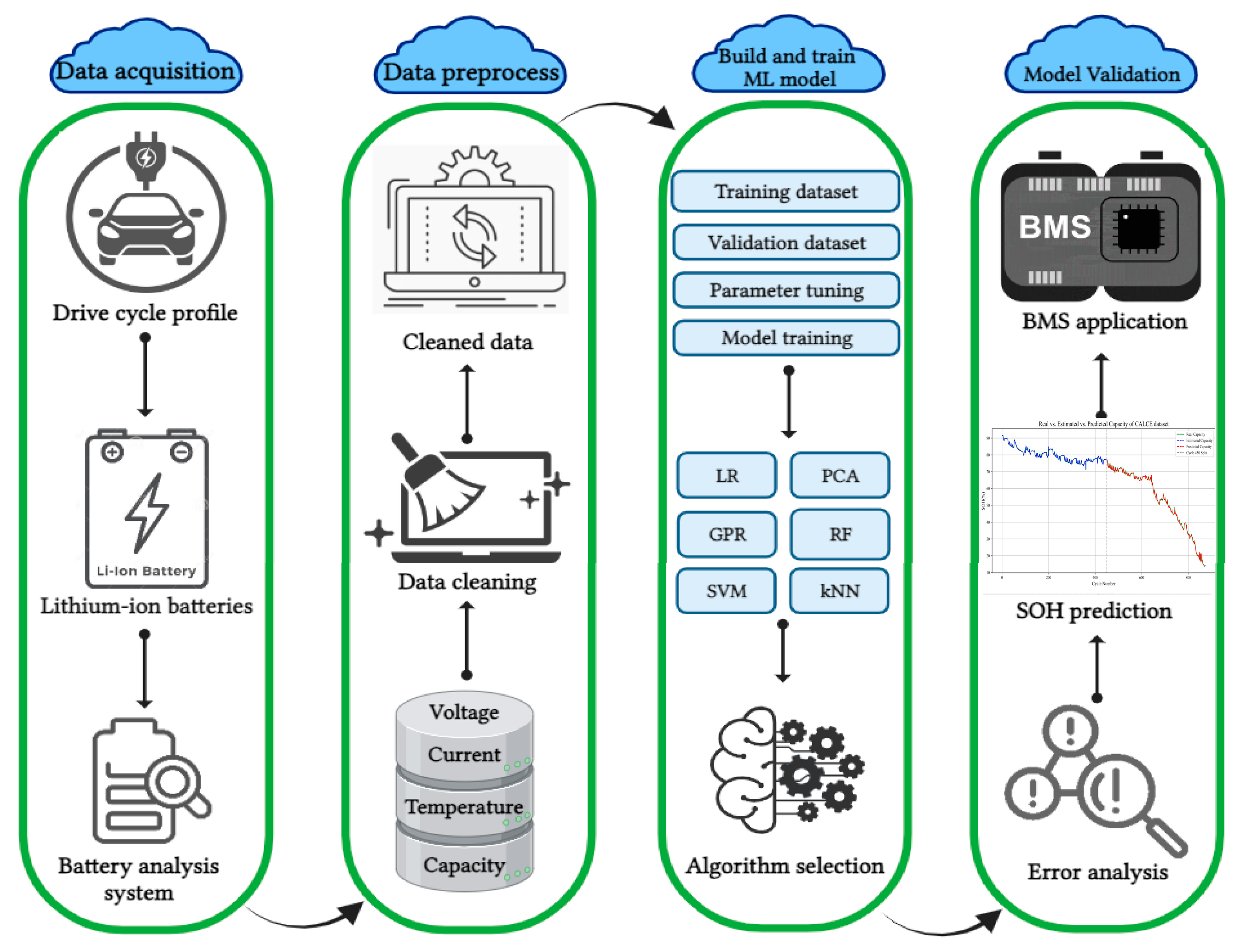
Both empirical experiments and physics-based modeling techniques require controlled conditions or complex testing scenarios [21,22]. Given the complexity of electrochemical mechanisms in LIBs, developing faithful physical models across different cell chemistries and formats can be difficult or infeasible in practice [23]. Moreover, such models depend heavily on substantial prior knowledge [24], and their outputs can vary widely with modeling assumptions and parameterization, limiting real-world applications. In contrast, data-driven approaches provide reasonably accurate SOH estimates without detailed knowledge of underlying physicochemical and electrochemical processes, operating directly on historical cycling and operational data readily collected by BMS sensors [25,26]. They are also generally more cost-effective to develop and maintain than model-based approaches. Typically, data-driven SOH estimation involves four stages: data acquisition, data preprocessing, model training, and model validation estimation (Figure 2).
Machine learning (ML) algorithms have emerged as a cornerstone of data-driven SOH estimation by enabling the extraction of meaningful signals from complex battery datasets, particularly those capturing time series of discharge current, voltage, temperature, and charge/discharge time durations [27]. Appropriately chosen ML models enable more accurate assessments of battery health attributes, specifically SOH [28]. Increasingly, hybrid approaches that combine multiple algorithms are being adopted to enhance accuracy, reduce bias and variance, improve adaptability, and support online execution. Furthermore, different base models capture distinct patterns, trends, and outliers in the data, enabling a more comprehensive and precise SOH estimation [29,30].
Health indicators (HIs) are quantitative measures that describe the current status, performance, and degradation behavior of LIBs. They are typically derived from measurable features such as voltage, current, temperature, impedance, and capacity [31]. Effective feature selection identifies the most relevant and informative indicators, thereby reducing data dimensionality, improving model interpretability, and eliminating redundant or uninformative features [31,32]. HIs with strong correlations with SOH significantly improve the precision and robustness of data-driven predictive models [14]. The effectiveness of feature selection pipelines hinges on two key factors: (i) whether the chosen HIs adequately capture the complex electrochemical degradation mechanisms evolving over time, and (ii) whether the machine learning model can fully utilize the information embedded in each feature [33,34]. A variety of HIs have been explored in data-driven SOH estimation, yielding varying levels of accuracy. Table 1 summarizes representative studies, including the employed HIs, corresponding ML algorithms, and best reported performances. In essence, current data-driven SOH estimation faces two core challenges: (1) selecting optimal SOH-correlated features that are truly predictive, and (2) avoiding information redundancy when combining multiple features.
Developing advanced feature fusion strategies that effectively integrate diverse features—while capturing complex aging phenomena and minimizing redundancy—is therefore a research direction for improving SOH estimation robustness and accuracy [50]. Strategically selected and fused health features can more efficiently reflect degradation trends and serve as reliable inputs for training SOH prediction models. Several studies in Table 1 leverage multiple battery features (e.g., voltage, current, and temperature data) recorded during charge–discharge cycles from different analytical perspectives. While recent studies [34,49,50,51] have investigated multi-view features and multi-model fusions to better exploit both the potential of feature sets and algorithms achieving the highest SOH estimation accuracies. However, these approaches suffer from overly complex fusion model structures, challenging hyperparameter tuning, and limited estimation precision.
To address these limitations, this study proposes a Feature Accretion Method (FAM), that progressively expands the feature set using four HIs: voltage (V), incremental capacity (IC), and coefficients of polynomial fit functions on IC (IC/V) and capacity (Q/V) curves. An extensive evaluation of various regression models was conducted, incorporating a novel feature engineering approach using HIs for model training to estimate the state of health (SOH). FAM differs operationally from recent hierarchical/stacking or feature-reuse approaches [35,42] in two main respects. First, whereas many prior methods either (a) focus on reuse or transformation of a single feature family (for example, polynomial Q–V coefficients) or (b) stack model outputs so that predictions of lower-level learners serve as inputs to higher-level learners, FAM instead systematically repurposes entire recorded signals as dense HI feature vectors (i.e., features-in → ensemble). Second, FAM implements an explicit accretion/ablation protocol that progressively adds HI families and quantifies the incremental predictive value of each family; this supports evidence-based selection of the final ensemble composition and improves interpretability. Following data cleaning, feature selection, and transformation on the CALCE [56] and Oxford datasets [57], four regression models including Support Vector Regression (SVR), Random Forest Regression (RFR), Gaussian Process Regression (GPR), Lasso, and Extra Trees Regression (ETR)—were evaluated enabling a systematic comparison of how the newly introduced features contribute to SOH estimation across. Notably, the proposed three-phase FAM consistently achieves superior performance, highlighting its potential for robust SOH estimation at each stage.
The organization of this paper is structured as follows: Section 2 describes data preparation and HIs extraction from voltage, incremental capacity, and fitting function polynomial coefficients, and enlightens the employed algorithms. Section 3 represents the proposed FAM approach. Section 4 presents the research results in the form of SOH estimation plots, comparative performance analysis of different models, and visualizations of the estimated SOH values. Finally, Section 5 concludes with key findings and insights.

2. Data Preparation and HI Extraction

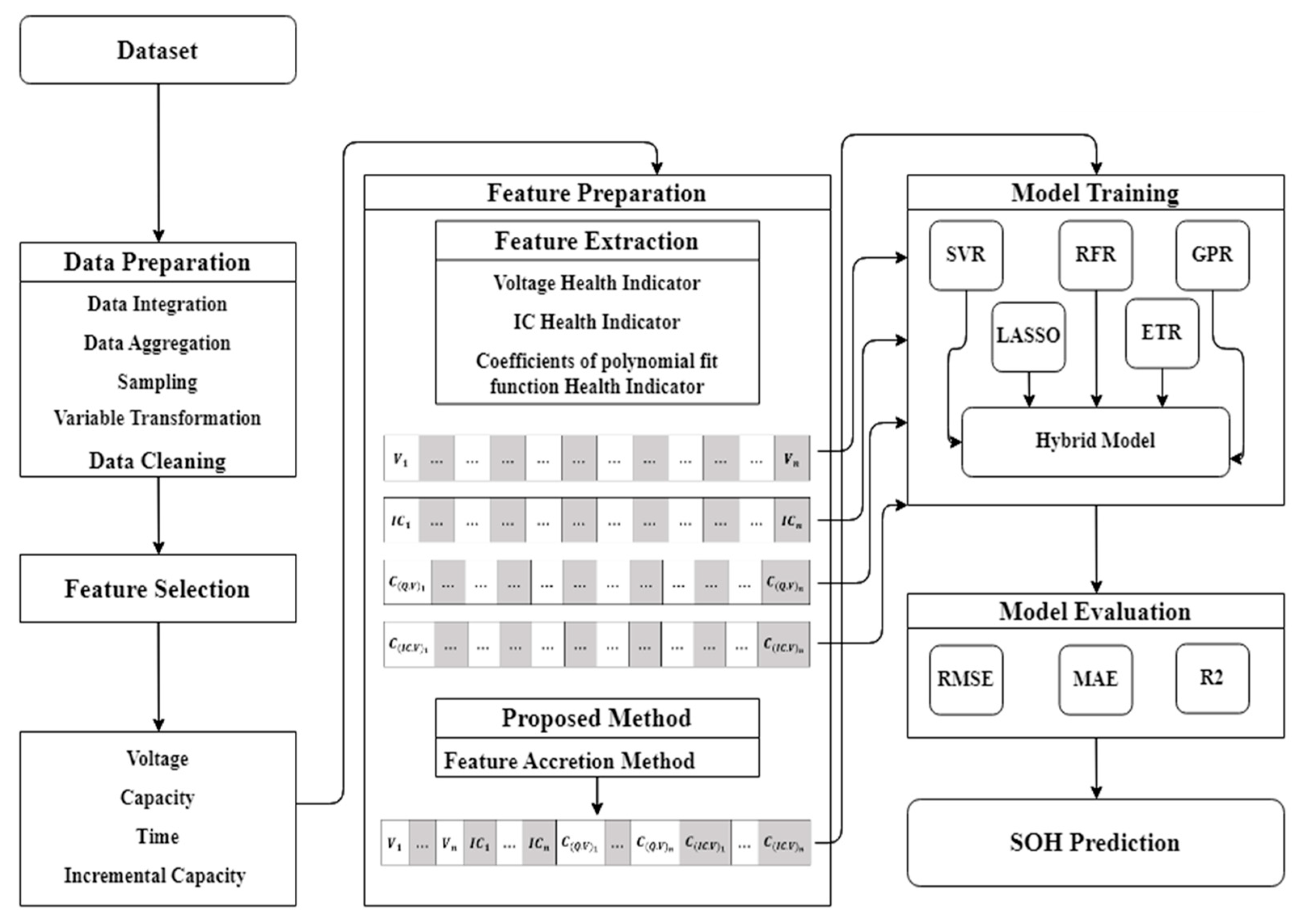
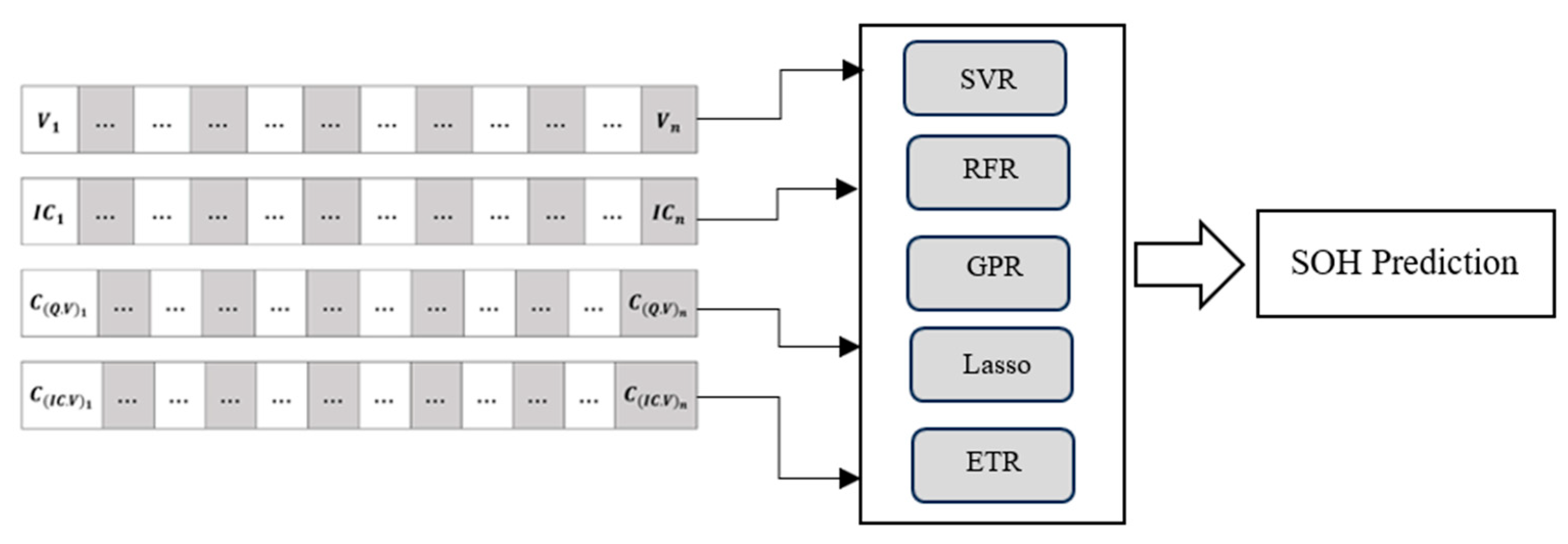
Figure 3 illustrates the overall workflow of the proposed Feature Accretion Method (FAM) for SOH estimation on the CALCE and Oxford datasets. The data preparation stage involved including integration, aggregation, sampling, transformation, and cleansing to ensure data quality and suitability for downstream analyses. From the processed datasets, key raw features—voltage (V), charge capacity (CC), time (T), and incremental capacity (IC)—were identified during the feature selection phase as primary inputs.
In the HI construction stage, which is critical in battery analytics, these features were transformed into four health indicators (HIs), including voltage (V), incremental capacity (IC), and coefficients of polynomial fit functions on IC (IC.V) and capacity (Q.V) curve variations. FAM proceeds in three phases. In the first, each HI was independently employed to train a standalone model. In the second phase, the most effective base learners are selected and integrated into an ensemble architecture. In the final phase, the proposed feature accretion method (FAM) resulted in HIs progressively accumulating as novel feature sets, which were then used to train models, yielding consistently improved predictive performance. Finally, the efficacy of the approach was rigorously evaluated using three metrics to substantiate the obtained results across both datasets.

2.1. Battery Data Set

Two publicly available datasets—Oxford and CALCE—were employed as case studies in the present research. The Oxford dataset comprises data from eight Kokam pouch cells (Cell 1–Cell 8). These cells were charged using a constant current of 2 C and discharged under the ARTEMIS Urban Drive Cycle. Capacity testing was performed every 100 cycles, at a 1 C charge–discharge rate. The CALCE dataset included batteries designated with serial numbers CS2-35 to CS2-38. A detailed summary of both analyzed datasets is presented in Table 2.
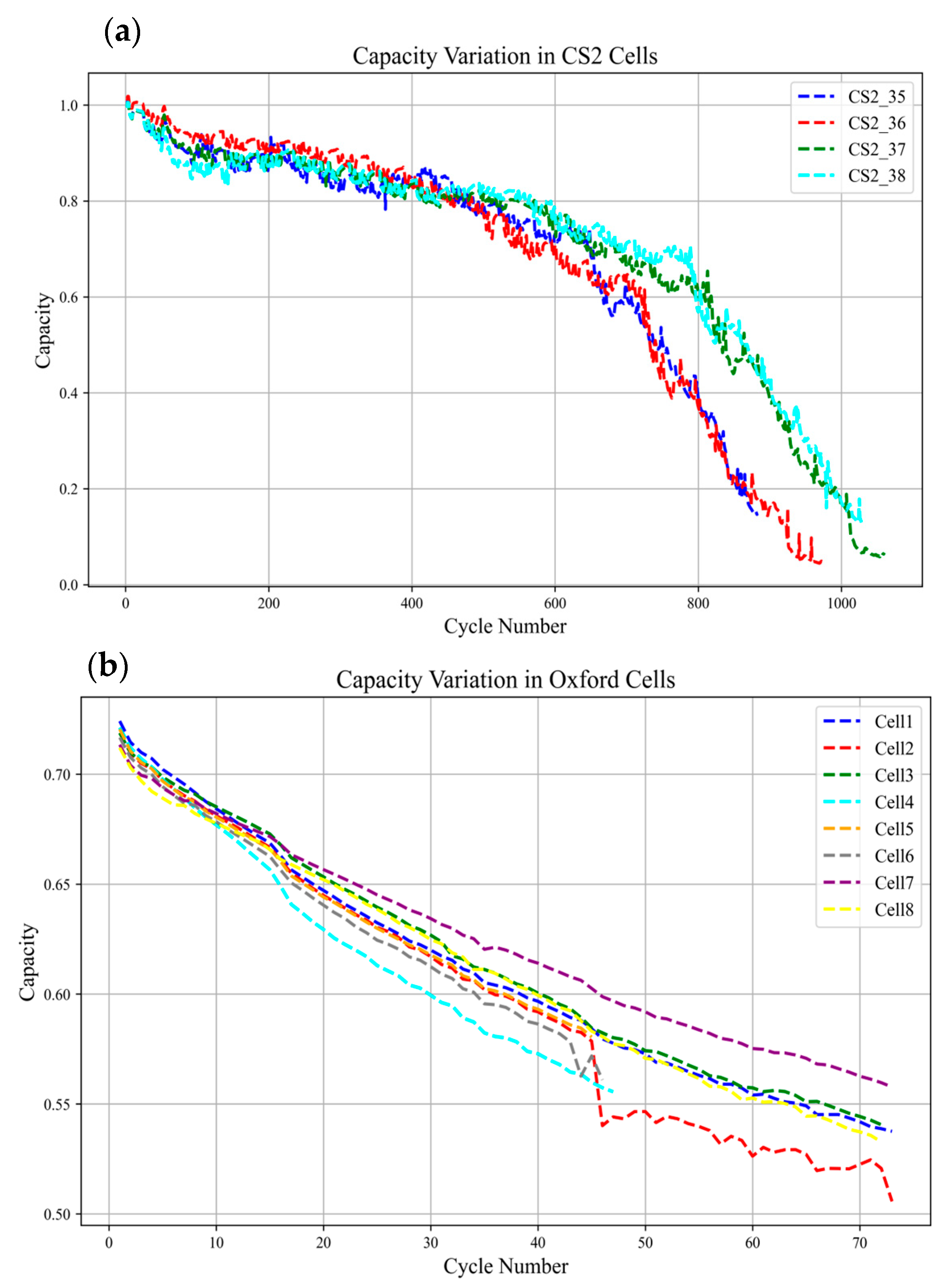
SOH degradation curves of representative cells of CALCE and Oxford datasets are shown in Figure 4. The results illustrate that SOH generally follows a gradual downward trend but also exhibits intermittent fluctuations. These fluctuations, often referred to as the capacity recovery phenomenon, typically arise during rest periods induced by Electrochemical Impedance Spectroscopy (EIS) tests or equipment shutdowns. Consequently, the battery degradation trajectory of LIBs involves both irreversible degradation (long-term capacity fade) and reversible degradation (temporary recoveries). To minimize the impact of these phenomena on SOH estimation, the following sections detail data processing procedures designed to improve the accuracy and robustness of SOH prediction.

2.2. Voltage Variation

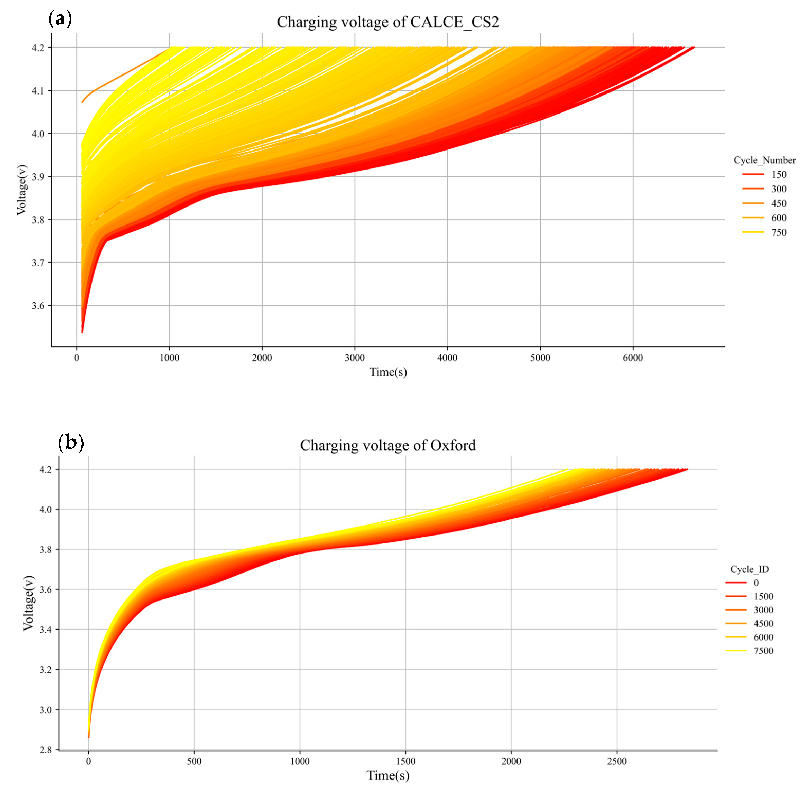
Figure 5 depicts the evolution of constant current (CC) charging voltage over time throughout the battery’s life cycle. As the battery ages, the voltage curve gradually exhibits a leftward shift, reflecting the progression of degradation. In the early life stages, the cell requires a longer duration to reach the upper cut-off (end-of-charge) voltage. However, with continued cycling, the time required to reach the cut-voltage progressively decreases. This shortened charging duration is closely correlated with capacity fade and thus serves as a reliable indicator of declining battery health.

2.3. Incremental Capacity Changes

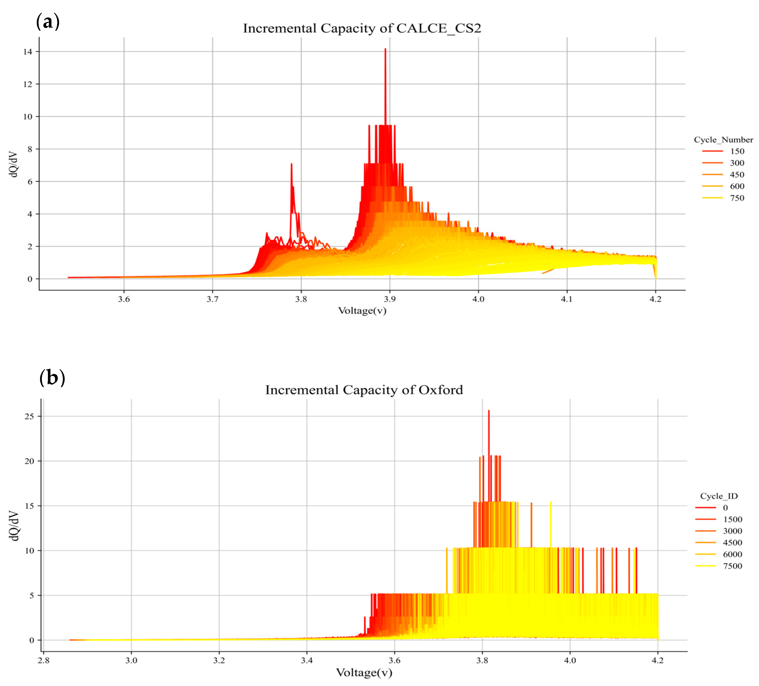
Incremental capacity (IC) analysis, which reflects the rate of change in battery capacity with respect to voltage, serves as a powerful diagnostic tool for continuous monitoring and a comprehensive understanding of LIB performance, facilitating in-depth evaluation. This method enables a detailed examination of the electrochemical behavior of LIBs, offering critical insights into their operational dynamics and health status. By carefully analyzing IC curves, researchers can detect subtle variations in cell behavior, which may include potential degradation mechanisms, such as capacity fade, electrode aging, or electrolyte decomposition. This early detection capability is essential for identifying emerging faults and developing targeted strategies to mitigate degradation, thereby enhancing maintenance and optimizing performance. Given its central role in assessing and predicting the estimation and prognostication of SOH, all IC-related data points are utilized as the training dataset for the models. Figure 6 illustrates the incremental capacity variation curves for both datasets.

2.4. Coefficients of Polynomial Fit Function in Capacity–Voltage Curve (Q.V)

In the lithium-ion battery research, polynomial fit functions are widely applied to model the complex relationship between the independent variable (voltage) and the dependent variables (charge capacity and incremental capacity). Such modeling not only enhances the understanding of battery behavior but also enables more accurate prediction of capacity from empirical data. Equation (1) represents the general formula of the polynomial fitting function.
f x = a 0 + a 1 x + a 2 x 2 + + a n x n
where x denotes the independent variable provided as an input vector, and f x represents the dependent variable.
The variation of capacity with respect to voltage plays a critical role in diagnosing and optimizing the performance and health of Li-ion batteries, thereby contributing to advances in battery technology and energy storage systems. In the third health indicator (HI), capacity was taken as the dependent variable and voltage as the independent variable for each cycle. Bai et al. [42] focused on forecasting the State of Health (SOH) by extracting energy features as health indicators and applied a sixth-degree polynomial fitting function to the voltage–capacity curve over time. Based on their findings, the optimal polynomial degree was determined to be six, a choice that captures the nonlinear nuances of battery behavior and enhances the accuracy of capacity estimation. To address the potential risk of overfitting given the relatively high-dimensional feature sets, we implemented multiple control analyses, including cross-validation, ablation, permutation importance, and variance inflation factor tests; see Supplementary Materials for details. Equation (2) represents the polynomial fitting function for the third health indicator.
Q i = c 0 + c 1 v i + c 2 v i 2 + c 3 v i 3 + c 4 v i 4 + c 5 v i 5 + c 6 v i 6
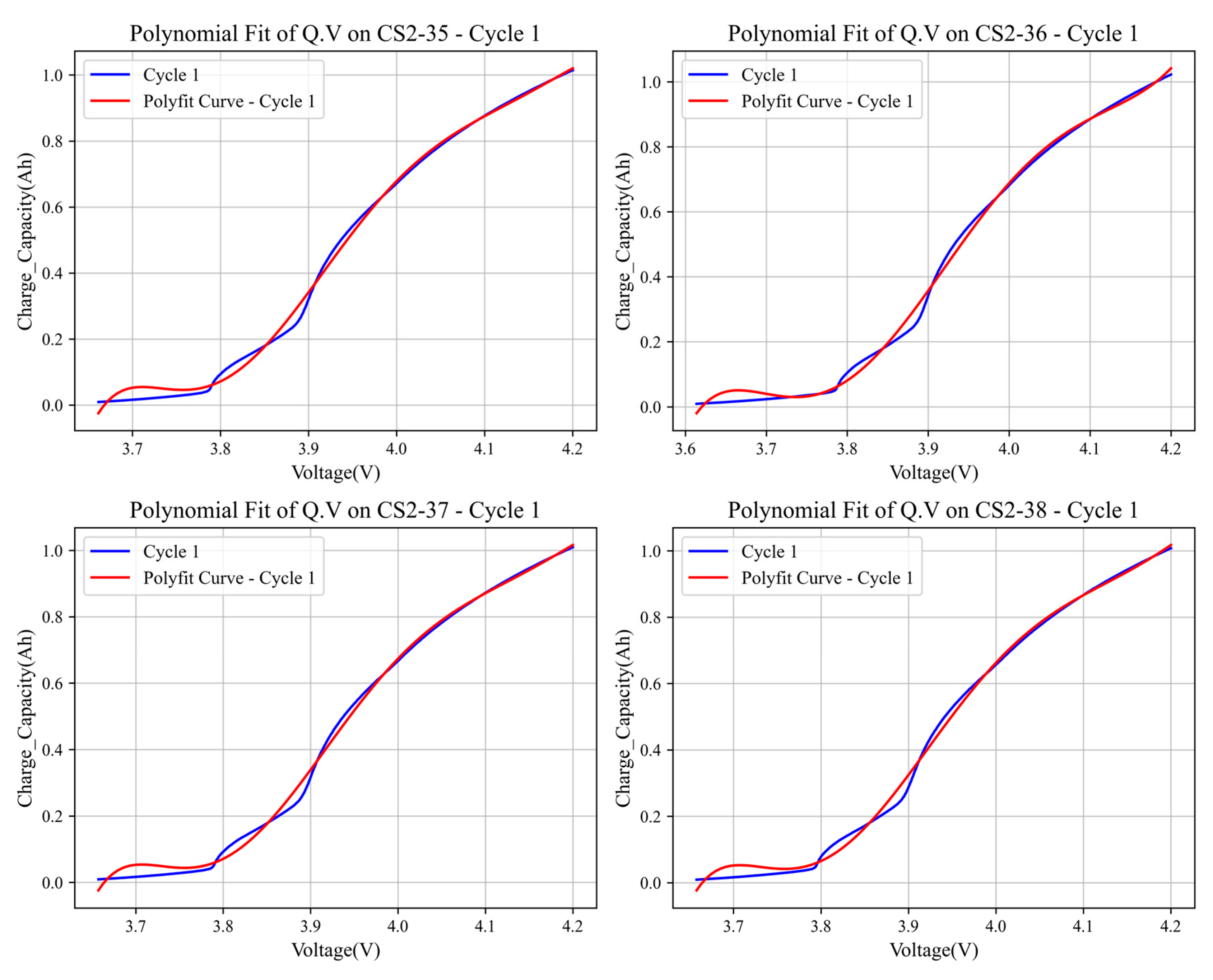
Figure 7 illustrates the capacity variation curve for a single cycle of the CALCE dataset, along with its sixth-degree polynomial fit spanning from the minimum to the maximum voltage. The coefficients derived from this polynomial function serve as novel features across all cycles.
The coefficients derived from this fitting function are extracted across all cycles and serve as novel features. This approach provides valuable insights into the dynamic interplay between capacity changes and voltage fluctuations throughout a complete cycle. By leveraging the fitted polynomial function, valuable coefficients were extracted, encapsulating essential information regarding the battery’s performance characteristics. These coefficients, integrated as new features, enrich our dataset, fostering a deeper understanding of battery behavior and facilitating advanced analytical methodologies.
Similarly, for the Oxford dataset, the coefficients obtained from the polynomial fitting function were utilized in the same manner as for the CALCE dataset. This methodological consistency ensured uniformity across both datasets, thereby enabling a robust comparative analysis of battery performance metrics. By incorporating these coefficients derived from the polynomial fitting function as components of the third and fourth health indicators, alongside the existing health indicators, we enhanced the comprehensiveness of the analytical framework. These coefficients serve as supplementary features that capture the interdependencies between voltage, capacity, and incremental capacity variations over time. Such a standardized approach not only streamlines the evaluation of battery behavior across diverse datasets but also strengthens the ability to identify subtle patterns associated with battery aging dynamics.

2.5. Coefficients of Polynomial Fit Function in Incremental Capacity–Voltage Curve (IC.V)

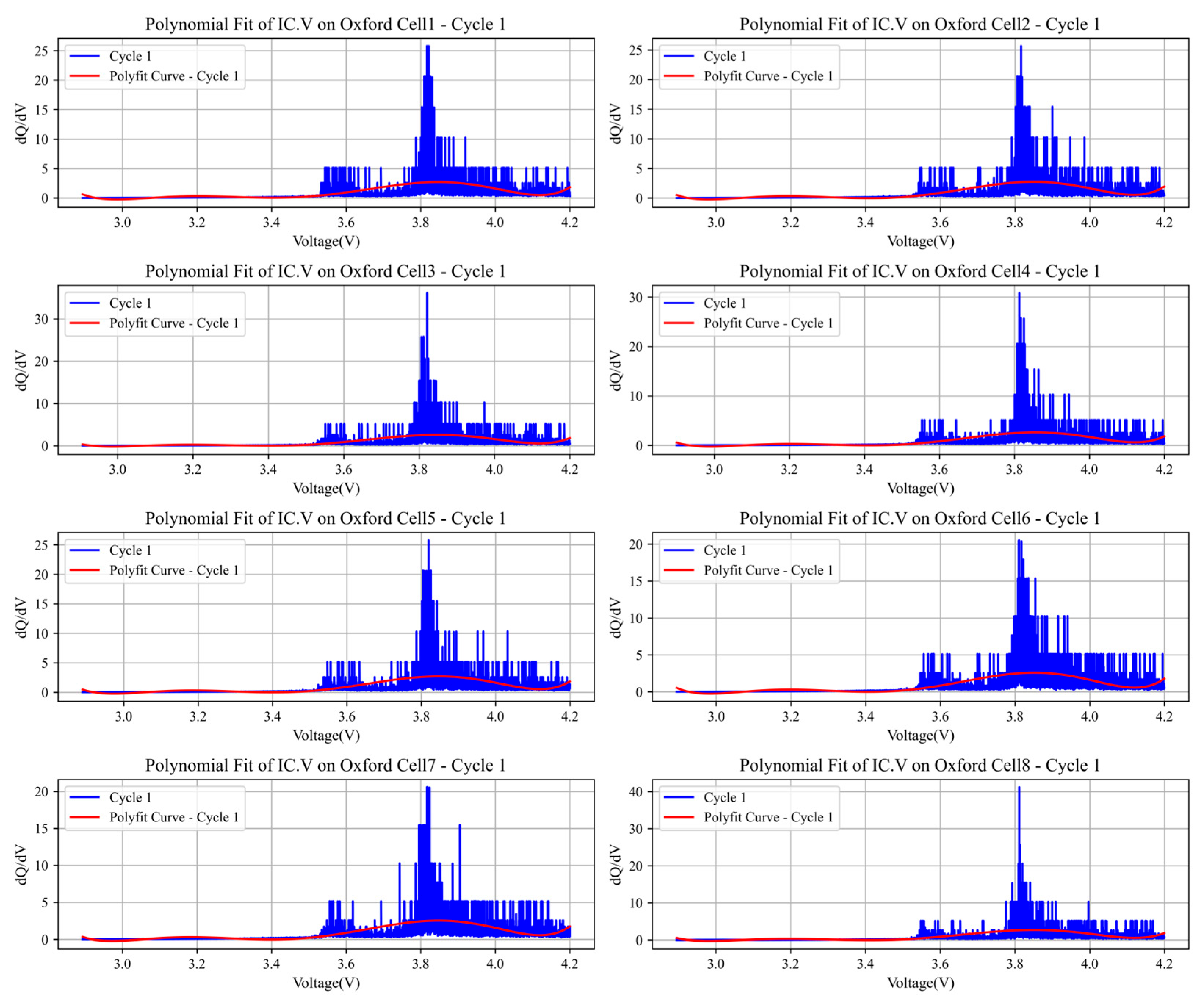
For the fourth health indicator, similar to the third health indicator, polynomial fitting function coefficients were again employed, analogous to the approach used in the third health indicator. The key distinction, however, lies in the utilization of the incremental capacity (IC) change curve rather than the capacity change curve. Figure 8 illustrates the IC change curve together with the fitted sixth-order polynomial for the Oxford dataset. The polynomial fitting function for the fourth health indicator is expressed in Equation (3), where voltage and IC were utilized as the independent and dependent variables, respectively.
I C i = c 0 + c 1 v i + c 2 v i 2 + c 3 v i 3 + c 4 v i 4 + c 5 v i 5 + c 6 v i 6
In Figure 8, although the fitted curves did not perfectly align with the target data, they yielded satisfactory results. The effectiveness of these curves can be attributed to the incorporation of fitted data during model training. By employing a polynomial fitting function to approximate the data, relevant information is captured from the target values, thereby enhancing the training process and influencing model performance. While alternative techniques, such as cubic spline interpolation, may provide more precise curve adjustments, the polynomial fitting remains a practical and effective approach for extracting valuable insights from the data.

2.6. Machine Learning Algorithm

The machine learning algorithms employed in this study included Support Vector Regression (SVR), Gaussian Process Regression (GPR), Random Forest Regression (RFR), Extra Tree Regression (ETR), and LASSO Regression. To optimize model performance, hyperparameter tuning was performed using Grid Search with parameter values adjusted according to the model type and dataset size.

2.6.1. Support Vector Regression (SVR)

Support Vector Regression (SVR) is a supervised learning algorithm designed for regression tasks. It functions by identifying a hyperplane in a high-dimensional space that best represents the data distribution. SVR aims to minimize prediction error while ensuring that deviations from the hyperplane remain within a defined threshold (margin). This approach is particularly effective for handling nonlinear and high-dimensional data. Notably, SVR can be implemented in both linear and non-linear modes depending on the choice of kernel function.
Linear support vector regression:
f x = w x + b
Nonlinear support vector regression (using kernel function)
f x = i = 1 N α i k x , x i + b
And the optimization problem is to minimize the following value:
1 2 w 2 + C i = 1 N ( m a x ( 0 , | y i f ( x i ) | ) ) 2
According to the limitation:
| y i f ( x i ) | ε
where w defines the weight vector, b represents the bias terms, k x , x i   is the kernel function that signifies the inner product between x and xi in a transformed feature space. C is a tuning parameter that trades off between a smooth decision boundary and a closely fitted one, controlling the training data. ϵ defines the epsilon-sensitive region, outlining the acceptable error margin. The solution involves finding support vectors, which are the data points lying on or at the margin’s fringe. The α i coefficients are determined during the optimization process and play a pivotal role in defining the regression function.

2.6.2. Gaussian Process Regression (GPR)

Gaussian Process Regression (GPR) is a Bayesian non-parametric regression technique that provides a probabilistic approach to modeling data. Unlike parametric methods, which assume a fixed functional form, GPR defines a distribution over possible functions, enabling both prediction and uncertainty quantification. This makes GPR particularly suitable for scenarios where noisy data or limited samples are present, as it naturally incorporates uncertainty in its predictions. Furthermore, the flexibility of GPR allows it to be applied effectively to both small- and large-scale datasets, making it a versatile tool in battery health estimation tasks.
f x ~ G P m x , k x , x ´ m x = m e a n   f u n c t i o n ,   k x , x ´ = c o v a r i a n c e   ( k e r n e l )   f u n c t i o n

2.6.3. Random Forest Regression (RFR)

Random Forest Regression (RFR) is an ensemble learning method built on decision trees and the bootstrap aggregating (bagging) principle. During training, it generates multiple decision trees using training and outputs the average prediction of individual trees. RFR is robust against overfitting and performs well with high-dimensional data. It is widely used due to its simplicity, scalability, and ability to handle both classification and regression tasks.
f x = 1 N i = 1 N T r e e i ( x )

2.6.4. Extra Trees Regression (ETR)

Extra Trees Regression (ETR) is an ensemble learning method closely related to Random Forests Regression (RFR). Like RFR, it constructs multiple decision trees using random subsets of training samples and features. However, ETR introduces an additional level of randomness by selecting split points entirely at random, rather than searching for the most optimal split. This increased randomness enhances diversity among the trees, often leading to improved generalization performance and reduced variance. Moreover, due to its simplified split-selection process, ETR is computationally more efficient, frequently achieving faster training times compared to RFR while maintaining competitive predictive performance.
y ^ = 1 N i = 1 N f i ( x )

2.6.5. LASSO Regression

LASSO (Least Absolute Shrinkage and Selection Operator) regression is a linear regression technique that incorporates regularization to improve model generalization. Specifically, it adds an L1L_1L1-norm penalty term to the Ordinary Least Squares (OLS) objective function, which not only constrains coefficient magnitudes but can also shrink some coefficients exactly to zero. It is particularly useful for sparse datasets with many features, as it helps prevent overfitting and improves model interpretability by reducing model complexity and mitigating multicollinearity.
J θ = 1 2 m i = 1 m ( h θ   x i y ( i ) ) 2 + α j = 1 n θ j

2.7. Evaluation Criteria

The effectiveness of the proposed State of Health (SOH) prediction models for lithium-ion batteries was evaluated using three statistical measures: Root Mean Square Error (RMSE), Mean Absolute Error (MAE), and R-squared (R2).
These metrics collectively assess the predictive performance of the models by quantifying the extent of prediction errors (RMSE and MAE) and the proportion of variance explained by the model (R2). Their use provides a rigorous evaluation framework, enabling the selection of optimal models, guiding hyperparameter tuning, and ensuring prediction reliability. This, in turn, supports informed decision-making for battery maintenance, repurposing, and facilitating benchmarking and comparison with previous studies. The use of these metrics provides a rigorous quantitative framework to evaluate and improve SOH prediction models, ultimately contributing to the advancement of battery management and utilization strategies.
R M S E = 1 N i = 1 N ( y i y ^ i ) 2
M A E = 1 N i = 1 N y i y ^ i
R 2 = 1 i = 1 N ( y i y ^ i ) 2 i = 1 N ( y i y ¯ i ) 2
In the context provided, N denotes the quantity of training or testing sample cycles. y i , y ¯ i , and y ^ i respectively signify the observed battery capacity, the mean capacity of the sampled cycles, and the anticipated battery capacity.

3. Methodologies of the Feature Accretion Method (FAM)

3.1. Individual Health Indicator-Based Battery Capacity Prediction

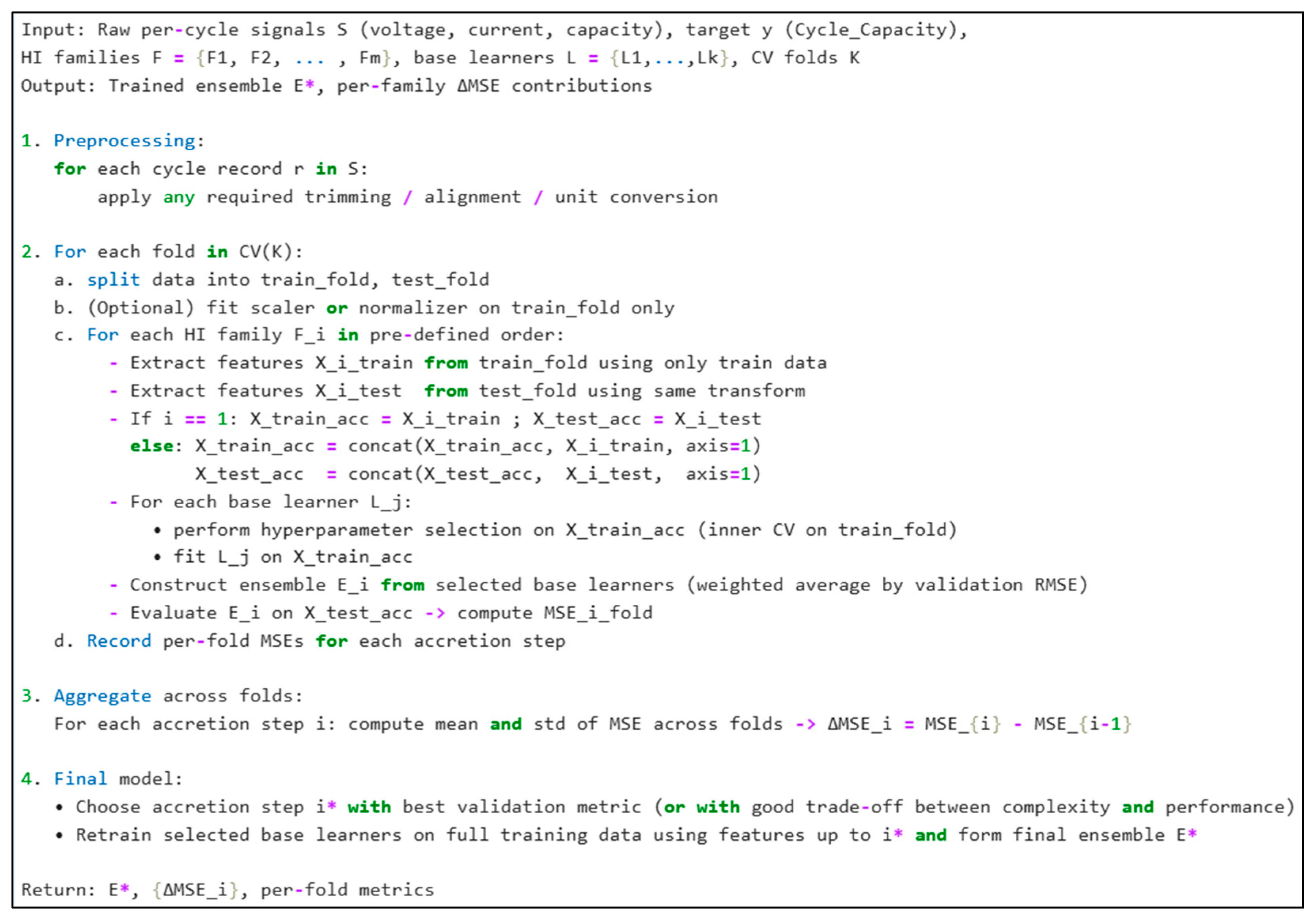
In the first phase of the proposed methodology, one or more features from the primary datasets were carefully selected and defined as health indicators (HIs). Unlike prior studies that typically employ derived statistical representations of these features, such as averages over specified intervals [56,58], peak values along the charge/discharge curve [13], differential voltage slope [59], or energy in the constant current and voltage charging stages [16], novel approaches were adopted. These approaches involved utilizing the full set of recorded data for each feature, followed by their transformation and integration into the modeling process as new features for training the desired models. This methodology ensures that no data is overlooked, maximizing the utilization of information closely aligned with the actual state of the battery, thereby improving the accuracy of SOH estimation. The complete step-by-step procedure of FAM, including preprocessing, feature accretion, ensemble evaluation, and model selection, is summarized in the pseudocode presented in Figure 9.
The features investigated included charging voltage (directly available from the dataset), incremental capacity (IC), and coefficients derived from a polynomial fitting function applied to both voltage–capacity and voltage–IC relationships. IC, in particular, reflects the changes in capacity corresponding to voltage variations within each cycle. To obtain the polynomial coefficients for the fitting function, as described in [42], a sixth-degree polynomial was employed. These coefficients were then integrated as new features, enhancing our ability to correlate them with battery capacity. Figure 10 illustrates the procedural framework adopted during this phase.

3.2. Dynamic Hybrid Model Health Indicator-Based Battery Capacity Prediction

Given the varying characteristics of the features extracted at each stage, it was inappropriate to employ a unified model encompassing the entire dataset with disparate features. Therefore, in this phase, a deliberate selection process was conducted to identify a suitable combined model that accommodates these features, considering their nature, quantity, and range. The models that performed the best in the previous step were chosen and integrated into the ensemble hybrid model. The performance of this ensemble model was evaluated while retaining feature-specific training sets, resulting in a significant improvement in outcomes.
Ensemble models operate by combining predictions from multiple individual models to enhance performance and overall results. This approach leverages the diversity of predictions from various models, often yielding superior outputs than individual models. A key advantage of ensemble models is their ability to reduce overfitting and improve robustness compared to standalone models. Figure 11 delineates the procedural framework adopted for the dynamic hybrid model HI-based battery capacity prediction. To assess prediction uncertainty, Gaussian Process Regression (GPR) was also applied in a supplementary analysis to generate ±2σ prediction intervals (Supplementary Materials Figure S1).

3.3. Feature Accretion Method-Based Battery Capacity Prediction

In this critical phase, which constitutes the primary objective of the final methodology, the health indicators were aggregated into a comprehensive training set and input into individual predictive models. Building upon insights gleaned from preceding stages, the most effective models were identified for incorporation into the ensemble model. By utilizing all health indicators as robust training sets, the hybrid model was constructed. Figure 12 illustrates the procedural framework employed for FAM-based battery capacity prediction. To diagnose potential redundancy among the extracted features, we additionally computed correlation matrices (Supplementary Materials Figure S2), PCA variance profiles (Supplementary Materials Figure S3), and variance inflation factors (VIF) (Supplementary Materials Figure S4). We further evaluated feature-level predictive contribution using permutation importance (Supplementary Materials Figure S5) and mutual information ranking (tracked ΔMSE at each accretion step) (Supplementary Material Figure S6).

4. Results and Discussion

Health indicators (HIs) serve as essential and pivotal components in battery-related research. As the field progresses, new methodologies are continuously introduced as health indicators [60]. The key challenge addressed in this study is to ascertain when it is more appropriate to utilize HIs individually and when the FAM method can yield superior outcomes. Specifically, this study investigates whether, in terms of computational complexity, time, and hardware requirements, researchers would derive greater benefits more from individual approaches or the proposed FAM method. Subsequently, a comparative analysis of the individual and aggregated methodologies introduced in this research is conducted to evaluate the findings.

4.1. Comparison of Individual Models with Hybrid Model

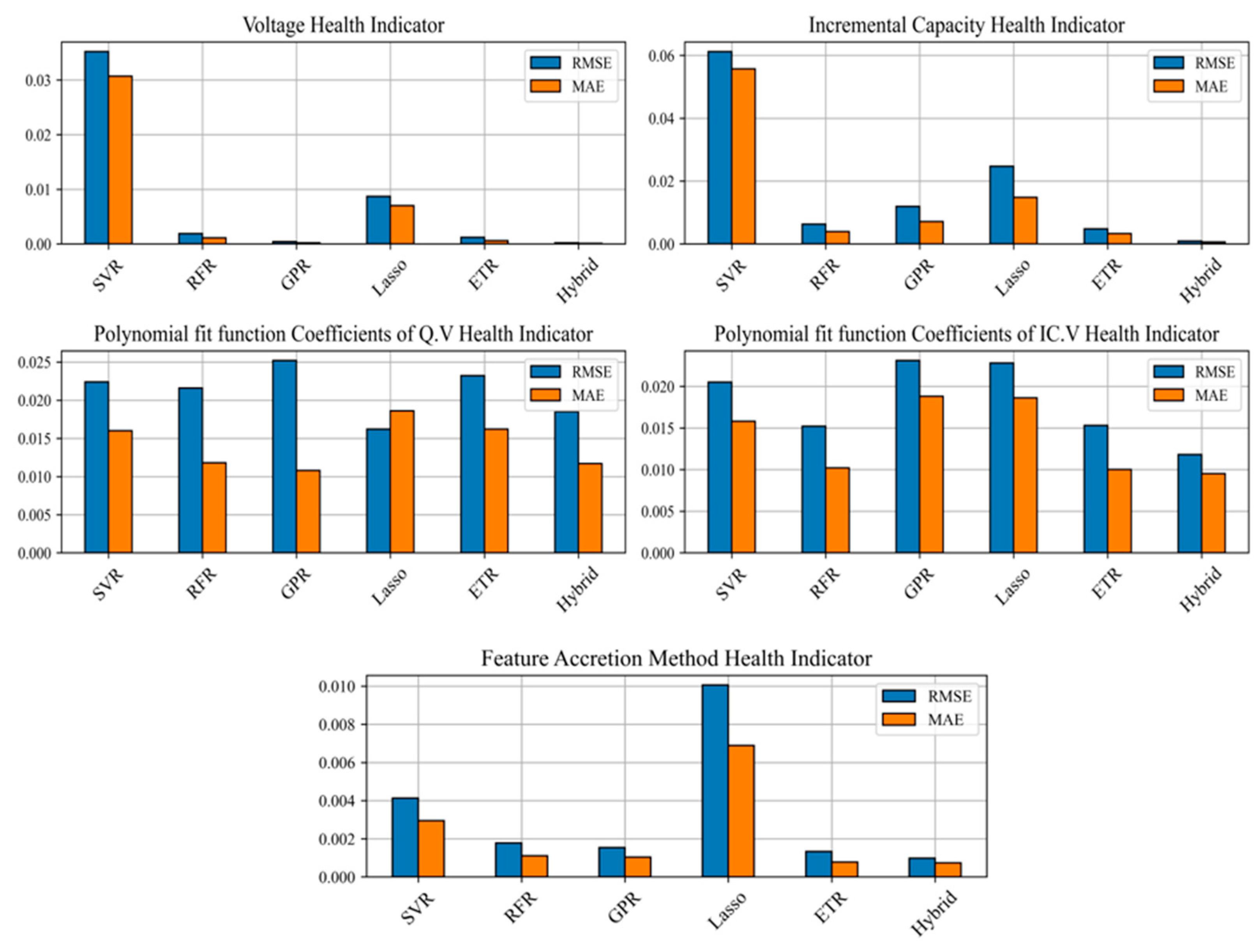
Among the models evaluated using the CALCE dataset, Gaussian Process Regression (GPR) exhibited the most favorable predictive performance when trained with the voltage health indicator, resulting in the lowest root mean square error (RMSE) of 0.0004, a mean absolute error (MAE) of 0.0002, and an R-squared (R2) value of 1.000. Notably, the Extra Trees Regression (ETR) model yielded superior performance with the incremental capacity (IC) health indicator compared to the other models. By employing the polynomial coefficients of the fitting function of capacity in relation to voltage as its training set, ETR surpassed the performance of alternative models. Similarly, Random Forest Regression (RFR) outperformed other models when trained with C(IC.V) as the fourth health indicator, highlighting the efficacy of decision tree-based models in estimating the state of health (SOH) in lithium-ion batteries (LIBs). Control analyses (see Supplementary Materials) further indicated that model performance did not depend on a single redundant feature group, and that predictive contributions were broadly distributed across HI families. Table 3 presents the outcomes achieved during phases one and two for the CALCE dataset.
Following the completion of the initial phase, the collective performance of the models during the training phase was assessed using distinct health indicators, with results documented accordingly. Notably, the combination of top-performing models yielded significant results, as evidenced by the highlighted findings in Table 3. The evaluation of the combined model utilizing the voltage health indicator resulted in an RMSE of 0.0002, an MAE of 0.0001, and an R2 value of 0.9999. When trained with the IC health indicator, the combined model achieved an RMSE of 0.0008, an MAE of 0.0005, and an R2 of 0.9999. Evaluation based on the third health indicator (C(Q.V)) yielded an RMSE of 0.0043, MAE of 0.0030, and an R2 of 0.9995. Finally, when assessed using the C(IC.V) health indicator, the implementation of the combined model resulted in an RMSE of 0.0118, MAE of 0.0095, and an R2 of 0.9964.
Based on the Oxford dataset, some results were analogous to those obtained from the CALCE dataset. GPR outperformed other models, exhibiting the lowest RMSE of 0.0017, an MAE of 0.0015, and an R-squared (R2) value of 0.9999 when trained with the voltage health indicator. The context of model training with IC revealed comparable performance for RFR and ETR. Employing polynomial coefficients of fitting functions as training sets for GPR and ETR proved to be more efficacious than alternative approaches.
Table 4 presents the results obtained during phases one and two for the Oxford dataset. The integration of models in the second phase, along with their training utilizing distinct health indicators, yielded promising results. The combined model trained with the voltage health indicator demonstrated an RMSE of 0.0016, an MAE of 0.0014, and an R2 of 0.9989. Similarly, training with the IC health indicator enabled the combined model to achieve an RMSE of 0.0074, an MAE of 0.0043, and an R2 of 0.9784. Furthermore, by leveraging the third health indicator (C(Q.V)), the combined model recorded RMSE values of 0.0020, MAE values of 0.0016, and an R2 value of 0.9986. Ultimately, employing the combined model with the C(IC.V) health indicator yielded an RMSE of 0.0026, an MAE of 0.0022, and an R2 of 0.9976.

4.2. Feature Accretion Method (FAM) of Single and Hybrid Models

Table 5 and Table 6 present the results obtained with the proposed model for both datasets. In the initial phase, individual models were evaluated utilizing novel features extracted from the accretion of four health indicators. Subsequently, in the principal phase of the proposed methodology, the optimal results achieved with individual models were amalgamated into an ensemble model. The outcomes of the ensemble model are indicated in bold font. Permutation-importance results (Supplementary Materials Figure S5) corroborate the ablation study by showing that predictive contributions are distributed across multiple HI families rather than dominated by a single indicator.
To evaluate the accuracy and robustness of the proposed model, 10-Fold Cross-Validation was employed. The dataset is divided into ten equal subsets (folds). In each iteration, one fold is used as the test set while the remaining nine folds are used for training. This process is repeated ten times so that every fold is used exactly once for testing.
The main reason for adopting this method is that a simple random split into training and testing sets may lead to unreliable evaluation, especially when the dataset is limited or unevenly distributed. In contrast, 10-Fold Cross-Validation reduces bias and variance in the evaluation and provides more stable and reliable results.
Since the developed model is based on an ensemble method, the use of cross-validation becomes even more important. Ensemble models generate the final output by combining the results of multiple base learners. To ensure generalizability and to prevent overfitting, it is necessary to assess the performance of the ensemble across multiple data partitions.
Table 7 presents the Mean Squared Error (MSE) values obtained for each fold. As can be seen, the error values are very small in most folds, indicating the high accuracy of the proposed model. Only in the tenth fold is a relatively larger error observed, which can be attributed to differences in the data distribution of that fold compared to the others.
In addition to the main ensemble results, we employed Gaussian Process Regression (GPR) as a supplementary analysis to quantify predictive uncertainty. For each cell trajectory, ±2σ prediction intervals were generated, providing a measure of confidence around the mean SOH predictions. As shown in Supplementary Materials (Figure S1), these intervals consistently encompassed the ground truth while remaining narrow, indicating stable model performance and robustness against measurement noise. Principal Component Analysis (PCA) of the feature sets (Supplementary Materials Figure S3) further revealed that a limited number of principal components explained more than 90% of the variance, suggesting that the predictive models rely primarily on the most informative features. Together, these analyses confirm that the proposed pipeline is both accurate and robust. We note that GPR was used exclusively for uncertainty assessment and stability checks; it was not included in the final ensemble model.

4.3. Comparison with Other Models

However, FAM shares conceptual elements with stacking and other multi-model fusion techniques, as noted above, its primary distinction is the feature-centric accretion and ablation protocol. To position FAM relative to existing work, we compare against representative recent multi-feature and stacking/feature-reuse methods reported in the literature (Bai et al., 2023 [42]; Lin et al., 2022 [35]; and the reports summarized in Table 8 and Table 9 for the CALCE and Oxford datasets, respectively).
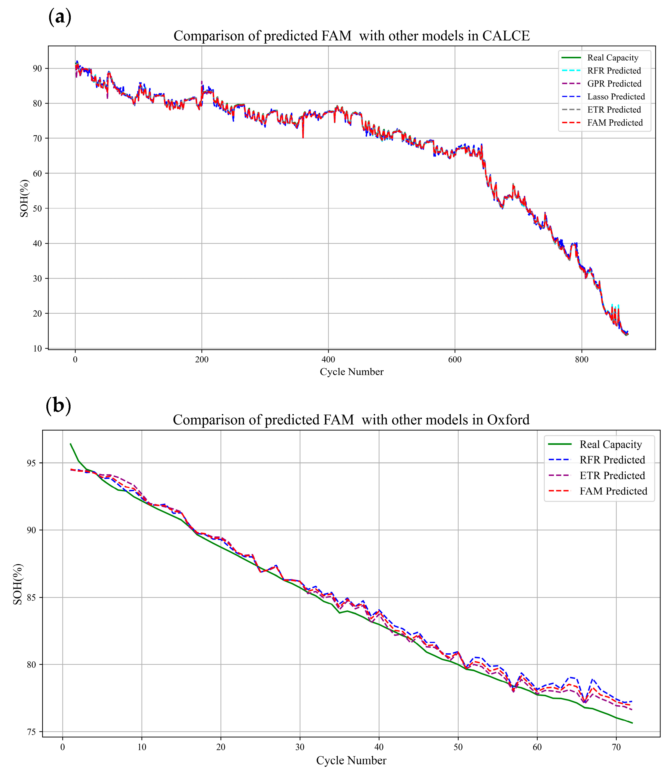
Upon analyzing the prediction outcomes presented in these tables, it is evident that the root mean square error of other algorithms in their optimal configurations is 0.69% for the CALCE dataset and 0.44% for the Oxford dataset. In contrast, the FAM yielded lower errors of 0.09% and 0.33%, respectively. Therefore, the proposed algorithm demonstrates superior accuracy. The ensemble model based on the feature accretion method can fully leverage the potential of features and significantly enhance prediction accuracy.

4.4. Analytical Evaluation of FAM on Existing Datasets

As discussed in Section 4.1, Section 4.2 and Section 4.3, the proposed model demonstrated significant results on the CALCE dataset. With the exception of the health indicator based on voltage, FAM outperformed the other individual health indicators. Although utilizing voltage alone as a health indicator resulted in lower error rates, relying solely on voltage without incorporating other influential factors in determining SOH provides limited insight. However, when combined with additional health indicators, voltage can serve as a powerful complementary factor to enhance prediction accuracy.
Concerning the Oxford dataset, while individual health indicators yielded superior results in certain instances, the performance of the proposed model exceeded the average results obtained from individual models and surpassed many models proposed in other referenced studies. Consequently, it can be argued that the proposed model exhibits enhanced performance across diverse datasets and demonstrates effective adaptability to varying data volumes and characteristics.

4.5. Discussion

To assess the proposed method with greater accuracy, we partitioned the entire dataset of each cell into a training set and a test set, designating one cell as the training set and another cell as the test set. The corresponding plots for each dataset are presented in Figure 13. In the case of the CALCE dataset, based on the box plots and frequency plots of different battery cells in both datasets, cell CS2-35 was utilized for training, while cell CS2-37 was employed for testing the models. For the Oxford dataset, cell number 8 served as the training set, and cell number 7 was utilized for testing. The predicted values generated by the proposed model demonstrate a superior fit compared to individual models. Although seven polynomial coefficients per curve could in principle lead to overfitting given ~100–300 cycles per cell, our control experiments (Supplementary Materials) showed that the pipeline’s cross-validation and feature selection steps controlled this risk effectively. On the other hand, together with the ablation ΔMSE analysis (Supplementary Materials Figure S7), permutation importance (Supplementary Materials Figure S5) demonstrates that each HI family provides incremental predictive value, supporting the design principle of feature accretion.
The GPR-based uncertainty intervals (Supplementary Materials Figure S1) demonstrated that predictions remain well-calibrated, while PCA confirmed that only a small subset of features is required, reducing the risk of overfitting. This performance edge stems from FAM’s progressive HI accretion and feature repurposing, which addresses limitations in prior hierarchical stacking methods (e.g., Bai et al., 2023 [42]; Lin et al., 2022 [35]) by enhancing interpretability and reducing redundancy, as evidenced by the lower RMSE (0.09% on CALCE) compared to benchmarks.
To clarify the physical relevance of the polynomial coefficients used as high-level health indicators, we note that a polynomial fit parameterizes the shape of the charge/discharge trace (Q–V) or its derivative (IC–V). The lower-order coefficients predominantly capture the global slope and curvature of the profile, reflecting bulk polarization and resistive/kinetic contributions of the cell. In contrast, higher-order terms represent localized inflections, shoulders, and peak structures associated with phase transitions or kinetics-limited plateaus. As degradation progresses, different electrochemical mechanisms alter these features in systematic ways: (i) loss of cyclable lithium shifts plateau positions and modifies the relative amplitude of dQ/dV peaks; (ii) impedance growth increases overall slope and broadens distinct features; and (iii) structural or phase changes adjust the sharpness and symmetry of local transitions. Consequently, variation in specific polynomial terms can be linked to underlying degradation processes—for example, increased cubic or quartic contributions often indicate peak broadening and plateau shifts, while changes in linear or quadratic terms are consistent with enhanced ohmic resistance. Thus, the degree-6 polynomial representation serves as a compact yet physically meaningful descriptor of capacity-fade-related phenomena.
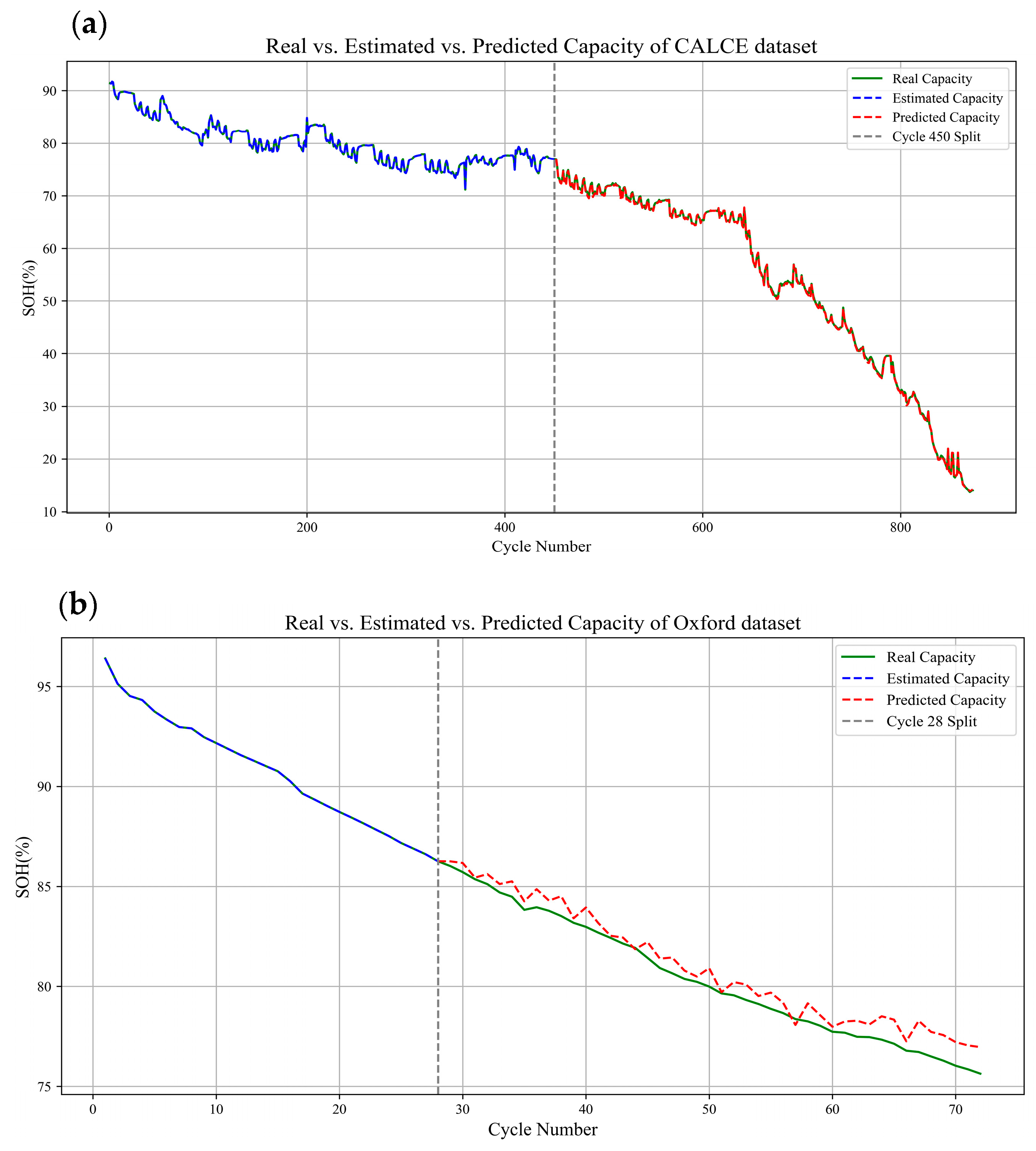
As shown in Figure 14, the predicted SOH is compared with the actual and expected values, thereby demonstrating the effectiveness of the suggested approach in forecasting or estimating the capacity of the Feature Accretion Method (FAM) for both the CALCE and Oxford datasets. The data presented underscores the efficacy and reliability of the FAM in accurately forecasting outcomes across diverse datasets, thereby highlighting its robustness and versatility in predictive modeling applications.
The bar plot depicted in Figure 15 elucidates the error values observed during phases two and three. Notably, it is evident that the combined approach of individual models consistently exhibits lower error rates across all stages and health indicators. Furthermore, the application of FAM results in a discernible reduction in the error rate, thus providing compelling evidence regarding the validity of the chosen approach.

5. Conclusions

While building on established feature fusion techniques, FAM’s innovations in systematic signal repurposing and empirical HI selection provide a practical advancement for SOH estimation, as validated on CALCE and Oxford datasets. In summary, the Feature Accretion Method (FAM) employed in this study offers an efficient approach for predicting battery health. Specifically, FAM achieved RMSE = 0.09%, MAE = 0.07%, and R2 = 0.9999 on the CALCE dataset and RMSE = 0.33%, MAE = 0.24%, and R2 = 0.9962 on the Oxford dataset. These values represent substantial improvements, with the CALCE case corresponding to an ≈87% relative reduction in RMSE compared with the best prior method (Table 7). By leveraging the complete data for each feature, FAM eliminates the necessity for complex preprocessing steps, thereby streamlining analysis and resource allocation. We extracted four health indicators pivotal for SOH estimation and utilized them to train our models individually. In the forward step, these HIs were accreted and utilized as new features for model training, with the main step applying this new training set in an ensemble model. The findings of this research provide a robust foundation for future advancements in battery health assessment. Moving forward, the integration of cutting-edge techniques such as dimensionality reduction and deep learning models holds promise for further improving predictive accuracy. Additionally, exploring refined fitting functions offers opportunities to optimize the reliability and efficiency of energy storage technologies. As we embark on future research endeavors, embracing these advancements will undoubtedly contribute to the evolution of battery health prediction, leading to more robust and effective solutions for the industry.

Supplementary Materials

The following supporting information can be downloaded at: https://www.mdpi.com/article/10.3390/en18195171/s1, Figure S1: GPR ±2σ prediction intervals. Gaussian Process Regression (GPR) results showing ±2σ prediction intervals around SOH trajectories; intervals consistently encompass ground truth, confirming calibration; Figure S2: Correlation heatmap. Heatmap of correlation coefficients among voltage samples, IC features, and polynomial coefficients, revealing clustering of related features; Figure S3: PCA cumulative variance plot. Cumulative explained variance of principal components, with >90% variance captured by a limited number of PCs, indicating effective dimensionality reduction; Figure S4: VIF values across feature sets highlighting multicollinearity among contiguous voltage samples; Figure S5: Ranked feature importance scores demonstrating distributed predictive contributions across heterogeneous HI families; Figure S6: Stepwise ΔMSE per accretion step. Mean squared error (MSE) changes as HI families are progressively added, quantifying incremental predictive value of each HI type; Figure S7: Ablation comparison (full vs. reduced feature sets). RMSE/MSE results before and after removal of correlated feature groups, confirming only modest loss in predictive accuracy.

Author Contributions

Conceptualization, L.A.; methodology, L.A.; software, L.A.; validation, L.A.; formal analysis, L.A.; investigation, L.A.; resources, A.S.; data curation, L.A.; writing—original draft preparation, L.A. and Y.V.; writing—review and editing, L.A., Y.V. and A.S.; visualization, L.A.; supervision, A.S.; project administration, L.A.; funding acquisition, A.S. All authors have read and agreed to the published version of the manuscript.

Funding

This research received no external funding.

Data Availability Statement

The original contributions presented in this study are included in the article/Supplementary Materials. Further inquiries can be directed to the corresponding authors.

Acknowledgments

We thank Sadegh Soleimany (University of Kurdistan) for their kind assistance.

Conflicts of Interest

The authors declare no conflicts of interest.

Abbreviations

The following abbreviations are used in this manuscript:
ETRExtra Trees Regression
FAMFeature Accretion Model
SOHState of Health
GPRGaussian Process Regression
RFRRandom Forest Regression
SVRSupport Vector Regression
ICIncremental Capacity
IC/QCoefficients of polynomial fit functions on IC
Q/VCoefficients of polynomial fit functions on capacity
CALCECenter for Advanced Life Cycle Engineering
BMSBattery Management System

References

  1. Nanaki, E.A.; Koroneos, C.J. Climate Change Mitigation and Deployment of Electric Vehicles in Urban Areas. Renew. Energy 2016, 99, 1153–1160. [Google Scholar] [CrossRef]
  2. Jeffry, L.; Ong, M.Y.; Nomanbhay, S.; Mofijur, M.; Mubashir, M.; Show, P.L. Greenhouse Gases Utilization: A Review. Fuel 2021, 301, 121017. [Google Scholar] [CrossRef]
  3. Ritchie, H.; Roser, M.; Rosado, P. CO2 and Greenhouse Gas Emissions. In Our World in Data; University of Oxford: Oxford, UK, 2020. [Google Scholar]
  4. Khatua, A.; Kumar, R.R.; De, S.K. Institutional Enablers of Electric Vehicle Market: Evidence from 30 Countries. Transp. Res. Part A Policy Pract. 2023, 170, 103612. [Google Scholar] [CrossRef]
  5. Costa, E.; Wells, P.; Wang, L.; Costa, G. The Electric Vehicle and Renewable Energy: Changes in Boundary Conditions that Enhance Business Model Innovations. J. Clean. Prod. 2022, 333, 130034. [Google Scholar] [CrossRef]
  6. Rouholamini, M.; Wang, C.; Nehrir, H.; Hu, X.; Hu, Z.; Aki, H.; Strunz, K. A Review of Modeling, Management, and Applications of Grid-Connected Li-Ion Battery Storage Systems. IEEE Trans. Smart Grid 2022, 13, 4505–4524. [Google Scholar]
  7. Sun, H.; Yang, D.; Du, J.; Li, P.; Wang, K. Prediction of Li-Ion Battery State of Health Based on Data-Driven Algorithm. Energy Rep. 2022, 8, 442–449. [Google Scholar]
  8. Han, X.; Garrison, J.; Hug, G. Techno-Economic Analysis of PV-Battery Systems in Switzerland. Renew. Sustain. Energy Rev. 2022, 158, 112028. [Google Scholar]
  9. See, K.W.; Wang, G.; Gandoman, T.S.; Van Mierlo, J.; Omar, A.; Van Den Bossche, F.; Omar, N. Critical Review and Functional Safety of a Battery Management System for Large-Scale Lithium-Ion Battery Pack Technologies. Int. J. Coal Sci. Technol. 2022, 9, 36. [Google Scholar] [CrossRef]
  10. Tran, M.K.; Panchal, S.; Khang, T.D.; Panchal, K.; Fraser, R.; Fowler, M. Concept Review of a Cloud-Based Smart Battery Management System for Lithium-Ion Batteries: Feasibility, Logistics, and Functionality. Batteries 2022, 8, 19. [Google Scholar] [CrossRef] [PubMed]
  11. Feng, X.; Weng, C.; He, X.; Han, X.; Lu, L.; Ren, D.; Ouyang, M. Online State-of-Health Estimation for Li-Ion Battery Using Partial Charging Segment Based on Support Vector Machine. IEEE Trans. Veh. Technol. 2019, 68, 8583–8592. [Google Scholar]
  12. Yang, S.; Liu, X.; Li, S.; Zhang, C. Advanced Battery Management System for Electric Vehicles; Springer Nature: Berlin/Heidelberg, Germany, 2022. [Google Scholar]
  13. Lin, C.; Xu, J.; Mei, X. Improving State-of-Health Estimation for Lithium-Ion Batteries via Unlabeled Charging Data. Energy Storage Mater. 2023, 54, 85–97. [Google Scholar] [CrossRef]
  14. Jiang, Y.; Chen, Y.; Yang, F.; Peng, W. State of Health Estimation of Lithium-Ion Battery with Automatic Feature Extraction and Self-Attention Learning Mechanism. J. Power Sources 2023, 556, 232466. [Google Scholar] [CrossRef]
  15. Yu, Z.; Liu, N.; Zhang, Y.; Qi, L.; Li, R. Battery SOH Prediction Based on Multi-Dimensional Health Indicators. Batteries 2023, 9, 80. [Google Scholar] [CrossRef]
  16. Gong, D.; Gao, Y.; Kou, Y.; Wang, Y. State of Health Estimation for Lithium-Ion Battery Based on Energy Features. Energy 2022, 257, 124812. [Google Scholar] [CrossRef]
  17. Wang, F.; Zhao, Z.; Zhai, Z.; Shang, Z.; Yan, R.; Chen, X. Explainability-Driven Model Improvement for SOH Estimation of Lithium-Ion Battery. Reliab. Eng. Syst. Saf. 2023, 232, 109046. [Google Scholar] [CrossRef]
  18. Lipu, M.S.H.; Hannan, M.A.; Hussain, A.; Hoque, M.M.; Ker, P.J.; Saad, M.H.M.; Ayob, A. A Review of State of Health and Remaining Useful Life Estimation Methods for Lithium-Ion Battery in Electric Vehicles: Challenges and Recommendations. J. Clean. Prod. 2018, 205, 115–133. [Google Scholar] [CrossRef]
  19. Vennam, G.; Sahoo, A.; Ahmed, S. A Survey on Lithium-Ion Battery Internal and External Degradation Modeling and State of Health Estimation. J. Energy Storage 2022, 52, 104720. [Google Scholar] [CrossRef]
  20. Singh, S.P.; Singh, P.P.; Singh, S.N.; Tiwari, P. State of Charge and Health Estimation of Batteries for Electric Vehicles Applications: Key Issues and Challenges. Glob. Energy Interconnect. 2021, 4, 145–157. [Google Scholar] [CrossRef]
  21. Kim, T.; Adhikaree, A.; Pandey, R.; Kang, D.-W.; Kim, M.; Oh, C.-Y.; Baek, J.-W. An On-Board Model-Based Condition Monitoring for Lithium-Ion Batteries. IEEE Trans. Ind. Appl. 2019, 55, 1835–1843. [Google Scholar] [CrossRef]
  22. Schmitt, J.; Rehm, M.; Karger, A.; Jossen, A. Capacity and Degradation Mode Estimation for Lithium-Ion Batteries Based on Partial Charging Curves at Different Current Rates. J. Energy Storage 2023, 59, 106517. [Google Scholar] [CrossRef]
  23. Ang, E.Y.M.; Paw, Y.C. Linear Model for Online State of Health Estimation of Lithium-Ion Batteries Using Segmented Discharge Profiles. IEEE Trans. Transp. Electrif. 2022, 9, 2464–2471. [Google Scholar] [CrossRef]
  24. Huang, Z.; Xu, F.; Yang, F. State of Health Prediction of Lithium-Ion Batteries Based on Autoregression with Exogenous Variables Model. Energy 2023, 262, 125497. [Google Scholar] [CrossRef]
  25. Hoque, M.A.; Nurmi, P.; Kumar, A.; Varjonen, S.; Song, J.; Pecht, M.G.; Tarkoma, S. Data Driven Analysis of Lithium-Ion Battery Internal Resistance Towards Reliable State of Health Prediction. J. Power Sources 2021, 513, 230519. [Google Scholar] [CrossRef]
  26. Jiang, B.; Zhu, J.; Wang, X.; Wei, X.; Shang, W.; Dai, H. A Comparative Study of Different Features Extracted from Electrochemical Impedance Spectroscopy in State of Health Estimation for Lithium-Ion Batteries. Appl. Energy 2022, 322, 119502. [Google Scholar] [CrossRef]
  27. Lombardo, T.; Duquesnoy, M.; El-Bouysidy, H.; Årén, F.; Gallo-Bueno, A.; Jørgensen, P.B.; Bhowmik, A.; Demortière, A.; Ayerbe, E.; Alcaide, F.; et al. Artificial Intelligence Applied to Battery Research: Hype or Reality? Chem. Rev. 2022, 122, 10899–10969. [Google Scholar] [CrossRef] [PubMed]
  28. Zhao, J.; Xuebin, L.; Daiwei, Y.; Jun, Z.; Wenjin, Z. Lithium-Ion Battery State of Health Estimation Using Meta-Heuristic Optimization and Gaussian Process Regression. J. Energy Storage 2023, 58, 106319. [Google Scholar] [CrossRef]
  29. Shu, X.; Chen, Z.; Shen, J.; Shen, S.; Guo, F.; Zhang, Y.; Liu, Y. Ensemble Learning and Voltage Reconstruction Based State of Health Estimation for Lithium-Ion Batteries with Twenty Random Samplings. IEEE Trans. Power Electron. 2023, 38, 5538–5548. [Google Scholar] [CrossRef]
  30. Meng, J.; Cai, L.; Stroe, D.-I.; Ma, J.; Luo, G.; Teodorescu, R. An Optimized Ensemble Learning Framework for Lithium-Ion Battery State of Health Estimation in Energy Storage System. Energy 2020, 206, 118140. [Google Scholar] [CrossRef]
  31. Khaleghi, S.; Hosen, M.S.; Van Mierlo, J.; Berecibar, M. Towards Machine-Learning Driven Prognostics and Health Management of Li-Ion Batteries. A Comprehensive Review. Renew. Sustain. Energy Rev. 2024, 192, 114224. [Google Scholar]
  32. von Bülow, F.; Meisen, T. A Review on Methods for State of Health Forecasting of Lithium-Ion Batteries Applicable in Real-World Operational Conditions. J. Energy Storage 2023, 57, 105978. [Google Scholar] [CrossRef]
  33. Park, S.; Lee, P.; Kim, D.; Hong, S.; Na, W.; Kim, J. A SOH Estimation Method Based on ICA Peaks on Temperature-Robust and Aging Mechanism Analysis Under High Temperature. In Proceedings of the 2021 IEEE Applied Power Electronics Conference and Exposition (APEC), Phoenix, AZ, USA, 14–17 June 2021; pp. 2646–2649. [Google Scholar]
  34. Li, X.; Wang, Z.; Zhang, L.; Zou, C.; Dorrell, D.D. State-of-Health Estimation for Li-Ion Batteries by Combing the Incremental Capacity Analysis Method with Grey Relational Analysis. J. Power Sources 2019, 410, 106–114. [Google Scholar] [CrossRef]
  35. Lin, C.; Xu, J.; Shi, M.; Mei, X. Constant Current Charging Time Based Fast State-of-Health Estimation for Lithium-Ion Batteries. Energy 2022, 247, 123556. [Google Scholar] [CrossRef]
  36. He, Y.; Yang, J.; Chen, L.; Chen, Y.; Xu, B.; Hong, S.; Zhang, C.; Chen, N. State of Health Estimation of Lithium-Ion Battery Aging Process Based on Time-Frequency Fusion Characteristics. J. Power Sources 2024, 596, 234002. [Google Scholar] [CrossRef]
  37. Ji, S.; Zhu, J.; Lyu, Z.; Yuan, Y.; Yang, H.; Chen, Z.; Yang, X.; Li, P.; Shen, Y.; Hu, Y. Deep Learning Enhanced Lithium-Ion Battery Nonlinear Fading Prognosis. J. Energy Chem. 2023, 78, 565–573. [Google Scholar] [CrossRef]
  38. Wang, C.; Su, Y.; Ye, J.; Xu, P.; Xu, E.; Ouyang, T. Enhanced State-of-Charge and State-of-Health Estimation of Lithium-Ion Battery Incorporating Machine Learning and Swarm Intelligence Algorithm. J. Energy Storage 2024, 83, 110755. [Google Scholar] [CrossRef]
  39. Hu, W.; Zhang, C.; Liu, S.; Jin, L.; Xu, Z. Multi-Objective Optimization Estimation of State of Health for Lithium-Ion Battery Based on Constant Current Charging Profile. J. Energy Storage 2024, 83, 110785. [Google Scholar] [CrossRef]
  40. Li, X.; Yu, D.; Vilsen, S.B.; Stroe, D.-I. Accuracy Comparison and Improvement for State of Health Estimation of Lithium-Ion Battery Based on Random Partial Recharges and Feature Engineering. J. Energy Chem. 2024, 92, 591–604. [Google Scholar] [CrossRef]
  41. Zhang, Y.; Zhang, M.; Liu, C.; Feng, Z.; Xu, Y. Reliability Enhancement of State of Health Assessment Model of Lithium-Ion Battery Considering the Uncertainty with Quantile Distribution of Deep Features. Reliab. Eng. Syst. Saf. 2024, 245, 110002. [Google Scholar] [CrossRef]
  42. Bai, J.; Huang, J.; Luo, K.; Yang, F.; Xian, Y. A Feature Reuse Based Multi-Model Fusion Method for State of Health Estimation of Lithium-Ion Batteries. J. Energy Storage 2023, 70, 107965. [Google Scholar] [CrossRef]
  43. Zhang, Z.; Cao, R.; Zheng, Y.; Zhang, L.; Guang, H.; Hong, S. Online State of Health Estimation for Lithium-Ion Batteries Based on Gene Expression Programming. Energy 2024, 294, 130790. [Google Scholar] [CrossRef]
  44. Ye, J.; Xie, Q.; Lin, M.; Wu, J. A Method for Estimating the State of Health of Lithium-Ion Batteries Based on Physics-Informed Neural Network. Energy 2024, 294, 130828. [Google Scholar] [CrossRef]
  45. Cai, L.; Stroe, D.-I.; Li, J.; Jiang, Y.; Li, X.; Yin, X.; Wu, J. Automatically Constructing a Health Indicator for Lithium-Ion Battery State-of-Health Estimation via Adversarial and Compound Stacked Autoencoder. J. Energy Storage 2024, 84, 110711. [Google Scholar] [CrossRef]
  46. Wang, L.; Jiang, S.; Mao, Y.; Li, Z.; Zhang, Y.; Li, M. Lithium-Ion Battery State of Health Estimation Method Based on Variational Quantum Algorithm Optimized Stacking Strategy. Energy Rep. 2024, 11, 2877–2891. [Google Scholar] [CrossRef]
  47. Zhang, Y.; Hu, Z.; Wu, T. A State-of-Health Estimation Method for Lithium Batteries under Multi-Dimensional Features. World Electr. Veh. J. 2024, 15, 68. [Google Scholar] [CrossRef]
  48. Ma, C.; Zhai, X.; Wang, Z.; Wang, H.; Yang, X. State of Health Prediction for Lithium-Ion Batteries Using Multiple-View Feature Fusion and Support Vector Regression Ensemble. Int. J. Mach. Learn. Cybern. 2019, 10, 2269–2282. [Google Scholar] [CrossRef]
  49. Tian, J.; Xiong, R.; Shen, W. State-of-Health Estimation Based on Differential Temperature for Lithium Ion Batteries. IEEE Trans. Power Electron. 2020, 35, 10363–10373. [Google Scholar] [CrossRef]
  50. Liu, G.; Zhang, X.; Liu, Z. State of Health Estimation of Power Batteries Based on Multi-Feature Fusion Models Using Stacking Algorithm. Energy 2022, 259, 124851. [Google Scholar] [CrossRef]
  51. Lin, M.; Wu, D.; Meng, J.; Wu, J.; Wu, H. A Multi-Feature-Based Multi-Model Fusion Method for State of Health Estimation of Lithium-Ion Batteries. J. Power Sources 2022, 518, 230774. [Google Scholar] [CrossRef]
  52. Chen, J.; Liu, Y.; Yong, J.; Yang, C.; Yan, L.; Zheng, Y. State of Health Estimation of Lithium-Ion Batteries Using Fusion Health Indicator by PSO-ELM Model. Batteries 2024, 10, 380. [Google Scholar] [CrossRef]
  53. Cai, X.; Liu, T. State of Health Prediction for Lithium-Ion Batteries Using Transformer–LSTM Fusion Model. Appl. Sci. 2025, 15, 3747. [Google Scholar] [CrossRef]
  54. Zhou, Y.; Zhang, C.; Zhang, X.; Zhou, Z. Lithium-Ion Battery SOH Estimation Method Based on Multi-Feature and CNN-BiLSTM-MHA. World Electr. Veh. J. 2024, 15, 280. [Google Scholar] [CrossRef]
  55. Yang, X.; Ma, B.; Xie, H.; Wang, W.; Zou, B.; Liang, F.; Hua, X.; Liu, X.; Chen, S. Lithium-Ion Battery State of Health Estimation with Multi-Feature Collaborative Analysis and Deep Learning Method. Batteries 2023, 9, 120. [Google Scholar] [CrossRef]
  56. Center for Advanced Life Cycle Engineering (CALCE), University of Maryland. Battery Data. Available online: https://calce.umd.edu/battery-data (accessed on 17 August 2025).
  57. Howey, D.; Birkl, C. Long term battery ageing tests of 8 Kokam (SLPB533459H4) 740 mAh lithium-ion pouch cells. In Oxford Battery Degradation Dataset 1; University of Oxford: Oxford, UK, 2017. [Google Scholar]
  58. Wang, Z.; Feng, G.; Zhen, D.; Gu, F.; Ball, A.D. State of Health Estimation of Lithium-Ion Batteries from Charging Data: A Machine Learning Method. In Proceedings of the IncoME-VI and TEPEN 2021; Mechanisms and Machine Science, Tianjin, China, 20–23 October 2021; Springer: Cham, Switzerland, 2023; Volume 117, pp. 707–719. [Google Scholar]
  59. Goh, H.H.; Lan, Z.; Zhang, D.; Dai, W.; Kurniawan, T.A.; Goh, K.C. Estimation of the State of Health (SOH) of Batteries Using Discrete Curvature Feature Extraction. J. Energy Storage 2022, 50, 104646. [Google Scholar] [CrossRef]
  60. Kostenko, G.; Zaporozhets, A. Transition from electric vehicles to energy storage: Review on targeted lithium-ion battery diagnostics. Energies 2024, 17, 5132. [Google Scholar] [CrossRef]
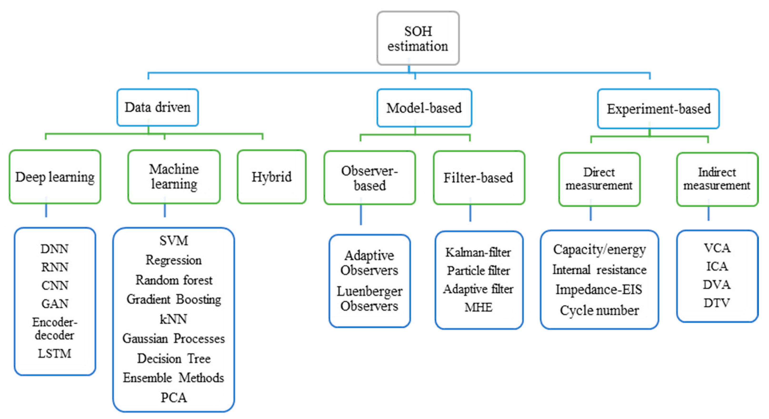
Figure 1. The classification of methods used to estimate SOH in Li-ion batteries (LIBs).
Energies 18 05171 g001
Figure 2. General pipeline of SOH estimation in Li-ion batteries with machine learning methods.
Energies 18 05171 g002
Figure 3. The workflow of SOH estimation based on the feature accretion method (FAM).
Energies 18 05171 g003
Figure 4. The capacity degradation curves: (a) CALCE dataset; (b) Oxford dataset.
Energies 18 05171 g004
Figure 5. Voltage variation over the life cycle: (a) CALCE dataset; (b) Oxford dataset.
Energies 18 05171 g005
Figure 6. Incremental capacity variations with voltage: (a) CALCE dataset; (b) Oxford dataset.
Energies 18 05171 g006
Figure 7. Polynomial fit function curve of charge capacity–voltage (Q.V) on CALCE dataset (Cells CS2-35 to CS2-38) in cycle 1.
Energies 18 05171 g007
Figure 8. Polynomial fit function curve of incremental capacity–voltage (IC.V) on Oxford dataset (cell 1 to cell 8) in cycle 1.
Energies 18 05171 g008
Figure 9. Pseudocode of the Feature Accretion Method (FAM). The algorithm details how health indicators (HIs) are concatenated, base learners are trained and weighted, and cross-validation is implemented to select the optimal ensemble.
Energies 18 05171 g009
Figure 10. Individual health indicator-based battery capacity prediction.
Energies 18 05171 g010
Figure 11. Dynamic hybrid model health indicator-based battery capacity prediction.
Energies 18 05171 g011
Figure 12. Feature Accretion Method (FAM)-based battery capacity prediction.
Energies 18 05171 g012
Figure 13. Comparison of the used models and FAM: (a) CALCE dataset; (b) Oxford dataset.
Energies 18 05171 g013
Figure 14. Comparison of the actual, expected, and predicted SOH: (a) CALCE dataset; (b) Oxford dataset.
Energies 18 05171 g014
Figure 15. The error values obtained in single models and the hybrid model on the CALCE dataset.
Energies 18 05171 g015
Table 1. An overview of the recently published literature related to SOH estimation, emphasizing employed algorithms, datasets, health indicators (HIs) and the best resulting performances.
MethodDatasetHIsBest PerformanceNumber of HIsRef.
KNN, SVR, NASA; CALCE; XJTU-EVCΔVstd, ΔVcharge-time; ΔVskewRMSE = 0.13%; MAE = 0.18%3[13]
RFROxford, CALCECCCTRMSE = 0.52%; MAE = 3.30%1[35]
GPR, SSGPR, BRR, LSSVRZenodoTime domain aging featuresRMSE = 0.58%, MAE = 0.70%13[36]
LR, RT, SVMNASA, CALCE, MITMechanistic feature empowerment of IC/QV/DV/ICDRMSE = 0.10%4[37]
CGM, SOA, GWO, IFA, PSONASA, Experimental datasetI, V, TRMSE = 0.92%, MAE = 0.75%3[38]
MOWOA-ELM, WOA-ELM, ALO-SVROxford, CALCEPolynomial fitting of constant current charging curvesRMSE = 0.58%, MAE = 0.44%4[39]
MLR, SVR, GPRExperimental datasetExtracted statistic features from partial recharging profilesRMSE = 0.29%15[40]
LSTM, DenseNet, CNN, ResNetNASACV, CCRMSE = 8.85; MAE = 7.92%2[41]
KNNR, ERTR, LoR, RFROxford, CALCEPIVT, TCCD, SampEn, TSVCRMSE = 0.16%, MAE = 0.14%4[42]
EN, LR, SVR, GPROxford, NASA, CALCE, MITEnergy-based features in CC, CV and EDVIRMSE = 0.06%, MAE = 0.05%3[16]
GEP, SVR, LSTMMITICA, DTVRMSE = 0.70%, MAE = 0.63%2[43]
PIFNN, FNN, CNN, RNNOxfordIC and DT based featuresRMSE ≥ 1%, MAE ≥ 0.5%2[44]
CNN, RNN, SVR, EVO-GPR, Encoder-DecoderNASA, MIT, Experimental dataReconstructed VRMSE = 0.63%, MAE = 0.51%1[45]
SVR, RF, XGBoost, Ridge, VQA-optimized stackingNASACapacity declined based HIsRMSE = 0.71%, MAE = 0.77%8[46]
POA-DELMNASAI, T, dQ/dVRMSE = 2.95%, MAE = 2.08%3[47]
AdaBoost and Stacking algorithmsNASADischarge-based features extracted based on SWBFERMSE = 0.29%, MAE = 0.31%12[48]
SVROxford, NASADT and ICA based extracted HIsRMSE = 0.23%, MAE = 0.90%21[49]
SVR, LSTM, Sta-ModelNASAExtracted HIs from CC-CV charging dataRMSE = 0.47%, MAE = 0.57%9[50]
MLR, SVR, GPROxfordV, T, and IC based HIsRMSE = 0.32%, MAE = 0.42%7[51]
PSO-ELMNASAvoltage interval time, avg voltage rise, CCCT, current diff, ICRMSE = 0.43%, MAE = 0.31%7[52]
Transformer-LSTMMITtime to cut-off V, CCCT, energy in CC discharge, EDVIRMSE = 0.13%, MAE = 0.10%10[53]
CNN-BiLSTM-MHAExperimental datasetIE, peak value, avg value, std, avg charging TRMSE = 0.21%, MAE = 0.17%5[54]
LSTMNASA, OxfordMulti-feature collaboration from DTV, SVD, ICA, TVCRMSE = 0.32%, MAE = 0.28%6[55]
Inputs: CCCT—Constant Current Charging Time; CCDC—constant current drop capacity; CCDT—Constant current drop time; CV—Constant voltage; CC—Constant current; PIVT—partial integration of voltage in time; TCCD—Time of constant current mode duration; SampEn—Sample entropy of discharge voltage; TSVC—The specific voltage band of the charging phase; EDVI—Equal Discharge Voltage Interval; ΔVstd—the standard deviation of voltage; ΔVskew—the skewness of voltage distribution; DT—Differential temperature; SWBFE—Sliding-window-based feature extraction technology; Models: RFR—Random Forest Regression; SSGPR—Sparce Spectrum Gaussian Process Regression; BRR—Bayesian Ridge Regression; LSSVR—Least Squares Support Vector Regression; LR—Linear Regression; LoR RT—Regression Tree; SVM—Support Vector Machine; SVR—Support Vector Regression; SOA—Seagull Optimization Algorithm; GWO—Grey Wolf Optimization; IFA—Improved Firefly Algorithm; MOWOA—Multi-Objective Whale Search Algorithm; ELM—Extreme Learning Machine; ALO—Ant Lion Optimizer; ResNet—residual Network; DenseNet—densely connected-convolutional networks; KNNR—K-Nearest Neighbor Regression; ERTR—Extremely Randomized Trees Regression; EN—Elastic Net; GEP—Gene Expression Programming; PIFNN—Physics-Informed Neural Network; FNN—Feedforward Neural Network; POA—Pelican Optimization Algorithm; GS—Grid Search; Sta-Model—Stacking Model.
Table 2. The overview of two battery datasets.
DatasetOxfordCALCE CS2
Number of cells84
From factorPouchPrismatic
CathodeLiCo2/LiNiMnCoO2LiCoO2
Capacity rating740 mAh1100 mAh
Voltage ranges2.7 V–4.2 V2.7 V–4.2 V
Depth of discharge 27.5 %   ±   0.5 %   to   21 %   ± 1% 100 %   to   69 %   ± 6%
ChargeCC (2C)CC-CV (1C)
DischargeArtemis urban driving cycleCC (1C)
Temperature 40   25  
Table 3. Individual and combined performance of models on CALCE data.
HIModelRMSEMAER2
VSVR0.03520.03070.9691
RFR0.00180.00110.9999
GPR0.00040.00021
Lasso0.00870.0070.9983
ETR0.00120.00061
Hybrid0.00020.00010.9999
ICSVR0.06120.05570.9065
RFR0.00630.00390.999
GPR0.01190.00710.9964
Lasso0.02470.01480.9848
ETR0.00480.00330.9994
Hybrid0.00080.00050.9999
C (Q.V)SVR0.01950.01530.9901
RFR0.01670.01090.9871
GPR0.02170.01780.9927
Lasso0.02820.02250.9792
ETR0.01590.01050.9934
Hybrid0.00430.0030.9995
C (IC.V)SVR0.02050.01580.9893
RFR0.01520.01020.9942
GPR0.02310.01880.9865
Lasso0.01860.02280.9869
ETR0.01530.010.9941
Hybrid0.01180.00950.9964
Table 4. Individual and combined performance of models on Oxford data.
HIModelRMSEMAER2
VSVR0.00390.00330.9946
RFR0.00310.00260.9961
GPR0.00170.00150.9999
Lasso0.00420.00330.993
ETR0.00360.00290.9946
Hybrid0.00160.00140.9989
ICSVR0.01640.01460.8943
RFR0.00760.00450.9772
GPR0.03570.02910.5022
Lasso0.02970.02530.6548
ETR0.00760.00450.9771
Hybrid0.00740.00430.9784
C (Q.V)SVR0.00560.00490.9898
RFR0.00440.00360.9936
GPR0.00230.00190.9983
Lasso0.00290.00230.9973
ETR0.00450.00350.9934
Hybrid0.0020.00160.9986
C(IC.V)SVR0.00570.00510.9893
RFR0.00460.00370.9931
GPR0.00260.00210.9978
Lasso0.01940.00610.993
ETR0.00450.00360.9931
Hybrid0.00260.00220.9976
Table 5. Performance of the Feature Accretion Method (FAM) on the CALCE dataset.
MethodModelRMSEMAER2
Feature Accretion Method
(FAM)
SVR0.00410.00290.9995
RFR0.00170.00110.9999
GPR0.00150.00100.9821
Lasso0.01000.00680.9973
ETR0.00130.00070.9999
Hybrid0.00090.00070.9999
Table 6. The performance of the Feature Accretion Method (FAM) on the Oxford dataset.
ModelModelRMSEMAER2
Feature Accretion Method
(FAM)
SVR0.01810.01170.8930
RFR0.00380.00270.9962
GPR0.03920.03140.4962
Lasso0.01060.00900.9633
ETR0.00380.00260.9951
Hybrid0.00330.00240.9962
Table 7. The 10-fold cross-validation was used to evaluate the robustness of the proposed FAM model on both the Oxford and CALCE datasets.
CALCE DatasetOxford Dataset
Fold NumberMSEMSE
F10.00066510.0009689
F23.2977 × 10−52.2845 × 10⁻⁶
F31.0361 × 10−51.8900 × 10⁻⁶
F43.6715 × 10−51.1490 × 10⁻⁶
F54.2694 × 10−57.7102 × 10⁻⁷
F61.9333 × 10−51.4898 × 10⁻⁵
F72.4105 × 10−51.4238 × 10⁻⁵
F82.0036 × 10−51.9672 × 10⁻⁵
F91.7701 × 10−57.3050 × 10⁻⁵
F109.9613 × 10−50.0203830
Table 8. Model performance comparison with other models on the CALCE dataset.
MethodRMSE (%)MAE (%)R2
FAM0.090.070.9999
[53]0.690.38-
[35]1.301.020.9425
[42]0.800.60-
Table 9. Comparison with other models on the Oxford dataset.
MethodRMSE (%)MAE (%)R2
FAM0.330.240.9962
[13]0.550.470.9646
[53]0.600.52-
[35]0.471.22 *-
[42]0.440.43-
* Maximum Absolute Error.
Disclaimer/Publisher’s Note: The statements, opinions and data contained in all publications are solely those of the individual author(s) and contributor(s) and not of MDPI and/or the editor(s). MDPI and/or the editor(s) disclaim responsibility for any injury to people or property resulting from any ideas, methods, instructions or products referred to in the content.