Article

Stochastic Markov-Based Modelling of Residential Lighting Demand in Luxembourg: Integrating Occupant Behavior and Energy Efficiency

Interdisciplinary Centre for Security, Reliability and Trust (SnT), University of Luxembourg, 1511 Luxembourg, Luxembourg
*
Author to whom correspondence should be addressed.
Energies 2025, 18(19), 5133; https://doi.org/10.3390/en18195133
Submission received: 5 September 2025 / Revised: 20 September 2025 / Accepted: 23 September 2025 / Published: 26 September 2025

Abstract

This study presents a stochastic Markov-based modeling framework for occupant behavior and residential lighting demand in Luxembourg. Integrating demographic data, time-use surveys, Markov chains, and dual-layer optimization, the model enhances the accuracy of non-HVAC energy demand simulations. The Harmonized European Time Use Surveys (HETUS) provide a detailed activity-based energy modeling approach, while Bayesian and constraint-based optimization improve data calibration and reduce modeling uncertainties. A Luxembourg-specific stochastic load profile generator links occupant activities to energy loads, incorporating occupancy patterns and daylight illuminance calculations. This study quantifies lighting demand variations across household types, validating results against empirical TUS data with a low mean squared error (MSE) and a minor deviation of +3.42% from EU residential lighting demand standards. Findings show that activity-aware dimming can reduce lighting demand by 30%, while price-based dimming achieves a 21.60% reduction in power demand. The proposed approach provides data-driven insights for energy-efficient residential lighting management, supporting sustainable energy policies and household-level optimization.

1. Introduction

More countries are trying to modify their energy systems to emit less greenhouse gases and run more sustainably, while still the global effort to combat climate change remains a critical concern. According to estimates, the building sector, comprising residential and commercial buildings, contributes a great deal to global consumption of energy and carbon emissions. In fact, buildings have been reported to account for an alarming 39% of all energy-related carbon emissions. In that percentage, the operational emissions from energy needed to heat, cool, and power the building make up the bulk, 28%, whereas the remaining 11% is contributed by materials and construction [1]. This significant effect underlines the necessity for action toward transforming built environments. Consequently, policy responses are oriented towards frameworks that focus on energy efficiency and sustainability [2]. Correspondingly, the European Union (EU) is committed to ambitious climate and energy targets in this regard. The EU has already enacted a greenhouse gas emission cut of at least 55% before 2030, in the context of its “Fit for 55” package, in contrast to 1990 levels, and a long-term goal is achieving climate neutrality by 2050 [3]. Attaining this goal will be supported by an EU building code encouraging energy effectiveness in buildings and forwarding an approach of net-zero energy buildings (nZEB) across the member states [4]. Each EU member country formulated its local, tailor-made action plans for the building sector aligned with different national conditions and tailored strategies meeting specific economic, climatic, and social contexts indigenous to each country. Decarbonization activities are targeted toward the introduction of renewable energy, electrification, and demand-side management (DSM) as primary strategies to meet these goals [2,3,4,5].

1.1. A Brief Review of Luxembourg’s Efforts in Residential Energy Efficiency and Sustainability

As a member of the European Union, Luxembourg is focused on regional energy objectives to alleviate households as well as making them as energy efficient as possible [6,7]. Public administration renovations would constantly involve the largest gap in the energy efficiency of existing building stock. Therefore, the government has acted to fast-track the renovation and to introduce smart technologies [8,9]. These are part and parcel of the future competition and climate-neutral economy [6,7,9,10]. In addition, Luxembourg has taken forward steps and introduced very strict laws to ensure that all new building construction must be nZEB compliant. A reflection of this commitment is “The Luxembourg Regulation on Building Energy Efficiency Update of June 2021,” which stipulates strict energy efficiency and decarbonized-heated systems, mostly heat pumps, for all new buildings [6]. The edict has changed since 2007 for houses and from 2010 for functional buildings, and this offers Luxembourg the luxury of positioning itself at the head of the pack in energy-efficient construction in Europe [6,7,9]. Recent statistics state that residential buildings consume about 21% of general energy consumption in the country [9]. For Luxembourg, the most important energy efficiency scheme is the Energy Efficiency Obligation Scheme (EEOS) [6], which was one of the strategic initiatives from Luxembourg to impart on energy efficiency. The scheme was established in 2015 and requires specific energy savings target achievements from energy suppliers. The cumulative energy savings target envisioned through the EEOS for the time period 2021–2030 is 42.54 GWh, or approximately 87.3% of the average final energy consumption in the country per the figures of 2016, 2017, and 2018 [6]. The “Klimabonus Wunnen” program, like the EEOS, incentivizes energy-efficient renovations in homes. The “Klimabonus Wunnen” program is a scheme offering financial incentives for energy-efficient renovations of residential buildings. It encourages homeowners to switch from fossil to renewable energy sources and improve the efficiency of their buildings [6]. An important aspect of the scheme is the introduction of pre-financing for climate subsidies, which just means citizens only pay for the portion of the investment that is not funded through the subsidy, thus making renovations easy, particularly for property owners who may not have the upfront capital necessary [6]. However, in addition to regulatory measures, understanding the behavior and energy usage patterns of household residents is crucial to designing effective, tailored policies [11,12]. In Luxembourg, besides other efforts, various initiatives have been developed to include building occupants in taking energy efficiency actions; one of the more prominent initiatives is the “LetzPower” project. Enabling residential consumers to have access to dynamic real-time energy data, including hourly prices and emission factors, “LetzPower” therefore empowers citizens to optimize their energy usage and align this with renewable generation, such as wind power. It reduces carbon footprints but, most importantly, instills a culture of informed and sustainable decision-making among consumers [13,14]. Effective policies for the energy transition require occupant-centric knowledge to bridge critical gaps in understanding residential energy behaviors. Technologies of metering and monitoring can provide insights into “how much” energy is used but not “why” or “how”, and thus, they leave large blind spots in household habits, socioeconomic characteristics, and the stochastic nature of energy use. This challenge is even more difficult because of privacy concerns and poor access to granular utility data, especially in Luxembourg, where most studies have been based on aggregated data or technical metrics, ignoring occupant-driven subtle energy behaviors [15,16]. The goal of achieving energy-efficient buildings in Luxembourg poses serious challenges due to a lack of holistic understanding in residential energy behaviors [6,7,9]. To tackle these issues, it becomes pertinent to have accurate modeling of household energy use that integrates diverse and dynamic habits of occupants. Accordingly, the next sub-section elaborates on how occupants can create energy demands and emphasizes on the role of behavior in energy simulation strategies.

1.2. The Role of Occupants in Building Energy Management

Continuing from the previous section, it will be important to note that in addition to the regulations, the occupant’s behavior is also crucial in formulating practical energy efficiency measures. Optimizing energy efficiency increasingly depends on the habits of occupants within the buildings [17]. Actions such adjusting of thermostats [18,19], opening window panes [20,21,22], or appliances’ usage [23,24], have their immediate effect on heating, ventilation, and air conditioning, indoor air quality, and energy consumption. The variability and unpredictability of occupant behaviors pose significant challenges for energy modeling and management, as they greatly influence the demands for heating, cooling, lighting, and ventilation [25]. Therefore, accurate simulation of such activities is a necessity for effective energy optimization [26]. Advanced sensing technology and real-time data-collecting gadgets could contribute to maximum understanding of the states and behavior of occupancy, while machine learning and stochastic approaches provide better predictions of these activities, resulting in more accurate simulation for energy management and better outcomes [11,21,27,28]. Moreover, integrating physiological and psychological aspects into simulations ensures that occupant comfort and satisfaction have been adequately sorted or taken into account [11]. As an example, including behavioral nuance gives more realistic consideration of conditions in simulation, enabling dynamic system adjustments that balance energy efficiency and occupant well-being [29,30]. Table 1 below compares three major modeling techniques: Stochastic Models, Deterministic Models, and Agent-Based Modelling (ABM). These techniques differ significantly in terms of complexity, predictability, data requirements, realism, general use cases, and computational burden, as well as their applicability across various scenarios. Deterministic models offer a simpler approach with low complexity and computational demands [31,32]. Fixed assumptions and schedules make such models capable of producing predictable results, which support simple simulation and building code compliance [32]. Deterministic models require minimal data and are thus efficient in computation, but they cannot formalize the dynamic, subtle interactions of occupants with their environment [32].
At a moderate to high complexity, stochastic models are designed to yield a number of different outcomes as a result of the incorporation of random elements [11,33]. These models, however, are the best at capturing occupant behavior’s variability and uncertainty and are therefore realistic [11,29,30,33]. The stochastic model consumes lots of data and also calls for intensive computation, hence limiting its practicality in certain situations [11].
Agent-based modeling (or ABM) is the most advanced and realistic modeling approach that simulates dynamic interactions between individual occupants and their environment [31,34]. It is highly realistic and covers different scenarios, but this would be achieved ideally in situations where occupants interact in a very complex way, such as during emergency evacuations or using spaces collaboratively [31]. Even though the above statements perhaps give a hint of the lengthiness of the required data and computational input, it can be possible that it may be resource-intensive for usage [31,34]. Choosing a modeling approach also depends on the simulation’s goals and limitations. For this work, we attempt to justify and utilize stochastic approaches to model occupant behavior, bringing in elements of inherent variability and uncertainty from what people do. By stochastic modelling, we aim to capture some of the more important contributions of occupant actions to variability regarding the energy performance of buildings while keeping the computational complexity manageable.

1.3. Relevant Studies

Stochastic models proffer reliable forecasts for building energy primarily predicated on occupancy behavior patterns. Most stochastic approaches (see Table 2) use Markov chains, which are the basic modelling approaches for occupancy behavior [35,36,37,38]. These methods have been well employed to construct high-resolution domestic activity and energy demand profiles, exploiting Time Use Survey (TUS) data to offer realistic representations of occupancy states [33]. Hence, the models not only represent daily variations and differentiate between and among different houses but also activity patterns through simulating probable transitions among the possible behavioral states [39]. The simplicity of the computation of Markov Chains makes them effective in capturing the stochasticity and time dependency associated with the behavior of the occupants [11,37,39]. TUS has also found a marked utility in stochastic models, particularly those involving Markov chains, as evidenced in the ample literature [40]. Markov chains apply probabilities of transition to emulate changes in behavioral states over time, while time-use data serve as the prime resource to calibrate these probabilities [11,40]. Capturing the detailed temporal pattern of daily activity, TUS is instrumental in creating models that simulate occupant behavior, including periods of activity, inactivity, and absence [12,33].
The TUS incorporates socio-demographic data such as age, income level, employment status, household size, and education level [40]. Social demographics in the TUS model energy-related behavior differences, for instance, household income differences, that exist within populations, for example, between low-income and high-income households [11,33,40,46]. One study uses American Time Use Survey (ATUS) data-based models that focus on occupancy schedules and occupant-driven energy simulations for city and national scales. The models are based on Markov chains and probabilistic methods that enable large-scale residential stock energy analysis within the United States [37,41]. Other studies integrated Canadian TUS data into stochastic load profile models of varying household archetypes [12,33]. These studies focus on lighting and domestic shower energy consumption, excluding energy used for space heating, such as cool or warm air [12,33]. For fine-grained predictions of space transitions and activity patterns at room levels, Danish TUS data are supplemented with Hidden Markov Models (HMM) in their development [38]. An example is undertaken in Belgium: TUS datasets have also been put to use for developing daily-to-day occupancy sequences with the intent of ensuring consistency in predictions for energy modeling through hierarchical clustering as proposed in [42]. Research in the United Kingdom shows examples of the applications that have been developed for state-transition modeling with Markov Chains (as in the Four-State Occupancy Model) and shows studies on the impact of temporal resolution for model accuracies for heating load and activity pattern simulations [35,43]. TUS are therefore an important set of data because they are regularly updated [40], thus ensuring that they would be valuable and useful for any research [11,40]. In addition, their national representative nature provides availabilities from a range of population categories, thereby presenting samples that can capture a considerable application area [5,21,35,36]. It spans various fields, including public health, transport, and economics, utilizing the data derived from the TUS [5]. It also enabled new applications such as demand flexibility modeling, mega cultural trend extrapolation studies, and energy policy formulation [12,33,46]. A common observation in the referenced studies is the simplification of the number of occupant states in modeling (normally reducing the number of states), often aimed at reducing the complexity of the analysis.
Markov chains and TUS data have also been used in the literature to support demand response. A mathematical model based on the Canadian profile generator was developed that looks at how household characteristics, among other factors, influence energy use and demand response [12]. It was also demonstrated how household diversity affects energy utilization, load cutting, and the advantages of the energy efficiency program. Furthermore, the Smart Grid Smart City (SGSC) trial, which was a large-scale trial project in Australia, was used to model DR participation by predicting household responses with the application of machine learning technology and stressing significant features and time series relations, thus highlighting the drivers of DR participation and enhancing program design through predictive models [45]. The socio-demographic data captured in TUS help in developing realistic, high-resolution simulations of daily activities that can be converted into energy. With its efficiency in capturing occupant behavior variability, Markov chains make the parties (households or energy providers) amenable to energy modeling, demand-side management, and energy policy decisions across the globe. But the use of this technique in measuring DR potential and residential power load flexibility is still fairly exploratory, probably because it requires too much data.

1.4. Research Contributions

The current study aims to close several gaps that exist in stochastic occupant modeling and for a more realistic DR and energy efficiency activities evaluation by combining a number of demographic datasets with stochastic models (Markov chain). The research enables the development of targeted energy strategies and paves the way for more inclusive, precise, and effective demand-side management practices. Important gaps include:
  • Most occupant modeling approaches reduce the number of occupant states. Even though such a simplification reduces the complexity of the computations involved, it decreases the possibility to formulate advanced power management strategies based on detailed, activity-based prioritization. Simplified models might fail in energy consumption optimization while cooking or during leisure activities, hence reducing their applicability and effectiveness. Therefore, such models may not handle complex energy needs of various occupant activities and hence provide less efficiency in general power management.
Contribution of the study:
Our primary contribution is a novel dual-layer optimization framework that enhances the behavioral realism of TUS-driven occupant profiles. The first layer uses Bayesian calibration to improve data alignment, while the second, constraint-based optimization layer enforces empirical time-use boundaries (e.g., plausible sleep or work durations). This integrated approach improves the accuracy of the generated profiles while maintaining the computational tractability of the Markov chain framework, addressing a key limitation of prior models.
2.
Few studies have explored the compatibility of TUS data with demand response (DR) and energy efficiency strategies, despite TUS being one of the most promising resources for advancing occupant modeling. This gap underscores the need for further research to fully characterize and design effective DR programs that harness the full potential of TUS data.
Contribution of the Study:
To address this gap, this study implements and analyzes several DR and energy efficiency programs using TUS data. The performance of these strategies in bridging the demand-supply gap of energy consumption is evaluated in conjunction with TUS-based occupant modeling. Especially with strategies like peak load period management and activity prioritization that match well with the developed model. Activity prioritization involves using lighting only during necessary activity and minimizing the energy use for nonessential activities to prioritize efficiently using TUS-derived activity patterns.
3.
Studies in Luxembourg have measured energy program participation by household type, ignoring the demographic and behavioral heterogeneity underlying energy consumption. Moreover, no comprehensive study in the literature creates a stochastic load profile generator that ties TUS data to final energy loads using available open-access data sources in Luxembourg. This gap shows the need for tailored, occupant-centric models that can precisely capture the complexities of residential energy behaviors in the region.
Contribution of the Study:
Our study tries to develop a holistic framework for the stochastic load profile generator by mapping occupant activities to final energy loads using open-access data for Luxembourg in Harmonized European Time Use Surveys (HETUS). We provide a Luxembourg-specific, data-driven method to improve local energy modeling accuracy.
4.
Our motivation for this research is to come up with a method of simplifying the constraints required so that TUS data can be directly loaded into a Markov-based model. Most conventional means of establishing stochastic occupant profiles with Markov chains showcase many demerits, like lack of flexibility to accommodate varying occupant behavior and extremely laborious manual intervention to match with real-world data.
Contribution of the Study:
Our contribution addresses this gap by introducing a dual-layer optimization approach that integrates with Markov-based models. By incorporating transition probability calibration and constraint-based optimization, our method enhances both data alignment with observed TUS patterns and behavioral realism in occupant profiles. This approach reduces the need for extensive manual adjustments, improves the model’s adaptability to varying occupant behaviors, and maintains computational efficiency.

1.5. Scope of the Work

This study develops a stochastic framework for modelling occupant behaviors and energy demand, focusing on residential buildings in Luxembourg and lighting power demand. We define the work scope and our initial assumption to define a clear work structure and give reader a true view about expected results and interpretation of developed method and results:
  • This work builds upon the methodologies of three seminal manuscripts [12,33,37] that address similar concepts and research questions, representing the forefront of knowledge in this field. While inspired by these studies, we have provided detailed explanations of all assumptions, methods, and results to ensure transparency and originality.
  • The term “stochasticity” in this context refers to the inherent variability in occupant behaviours over time, capturing day-to-day and week-to-week fluctuations. By employing a stochastic model, we can effectively represent both temporal variability and household heterogeneity, ensuring a more realistic depiction of behavioral dynamics, while accounting for demographic influences where applicable.
  • For the validation of power consumption, we referenced reported measured data from Eurostat [47] for annual lighting power demand across various countries, as well as available data specific to Luxembourg. Following established validation methods in the literature, we utilized average values to align with the assumptions underlying our stochastic simulation framework.
  • For the application of the proposed stochastic model, we focus on lighting power demand modelling in residential buildings. The model accounts for different lighting technologies, including LED, CFL, and incandescent bulbs, each with distinct energy consumption characteristics. To evaluate potential energy-saving opportunities, we investigate two energy efficiency measures: reducing lighting power based on occupant activities and daylight availability and dimming based on electricity price signals.
  • The applied household typology and demographic representation is in line with the existing literature, we define five major household types to capture the diversity of residential living arrangements in Luxembourg. To ensure accurate representation, we utilize data from the Luxembourgish census to estimate the relative share of each household type within the population.
  • We maintain relying on measured data from HETUS for Luxembourg and look to avoid self-assumptions when determining occupant behavior.
The rest of this work is structured as follows. Section 2 provides details about the applied datasets and essential definitions. Section 3 outlines the methodology, including the stochastic approach and DR strategies. Section 4 discusses the results obtained, and in Section 5 we will discuss the methodology, results, and work limitations. Section 6 draws conclusions of the main outcomes of this paper.

2. Harmonized European Time Use Surveys

The Harmonized European Time Use Surveys (HETUSs), in this study, are a procedure that is used in order to get information on what people are doing each day [48]. Through sketches, questionnaires, or interviews, HETUS acquires systematic data on activities such as personal care, occupation, recreation, housework, and travelling. These polls are used to understand human behavior, socio-economic trends, and lifestyle models, thus being a greatly important tool for sociology, economics, and urban planning investigations [33]. HETUS captures activity duration (spent time) and initiation time (start time), providing a structured view of daily routines [5].

2.1. Activity Classification and Coding Logic for Time Use Analysis

The actual activity of classification for time use analysis is a systematic activity and a hierarchical one: it attempts to bring about universal cross-comparability across datasets in terms of thematic alignment and consistency [5]. The activity classification made in “Detailed activity taxonomy for time use classification” (see Table S1) is derived from a framework complete in the sense of capturing all human activities in a structured manner.
HETUS classifies daily activities into broad themes like personal care, work, household tasks, and leisure, ensuring consistency across datasets (see Table S2) [5,48]. For example, the bulk activities category includes essential activities like “Sleeping” (AC01) and “Personal grooming” (AC0). In the household and family care category, activities like “Dishwashing” (AC31A), “Ironing” (AC331), and “Childcare” comprise (AC38A, AC38B) [5]. Each of the categories in the high-level taxonomy is made such that it groups activities meaningfully and coherently:
  • “Personal care except eating” includes activities dedicated to self-care, excluding food consumption. Tasks such as grooming, hygiene, and sleeping reflect foundational aspects of personal maintenance.
  • “Eating” represents a single, essential activity focused solely on food consumption, highlighting its central role in daily life.
  • “Work and study” encompass professional and academic pursuits, including employment tasks, studying, and related travel. These activities share a structured purpose, emphasizing their role in skill development and socio-economic engagement.
  • “Household and family care and related travel” groups activities aimed at managing and maintaining households, supporting family members, and associated mobility. Tasks such as cleaning, shopping, childcare, and related travel reflect the breadth of household responsibilities.
  • “Leisure, social and associative life except TV and video” highlights recreational activities, hobbies, and cultural participation that do not involve television. It includes active and social pursuits such as sports, games, and visiting with friends, showcasing the diverse ways people engage in leisure.
  • “Television and video” is a distinct category focused exclusively on screen-based entertainment, reflecting its unique role in modern recreational habits.
  • “Travel to/from work/study” includes commuting and academic travel, emphasizing the functional purpose of mobility in daily routines.
  • “Unspecified time use and travel” serves as a flexible grouping for undefined activities or ambiguous time use, ensuring comprehensive coverage of all recorded tasks.

2.2. Applied Datasets Overview

Continuing from Section 2.1, the discussed HETUS categories are available for different demographic groups in the HUTUS framework. These groups are presented in Table 3. Households are classified based on size, employment status, and education levels, ensuring demographic representation in the model.

2.3. Luxembourg CENCUS Overview

The 2021 census in Luxembourg revealed significant trends in employment and economic activity [49]. Among the 591,630 respondents, 48.5% were employed, up from 43.2% in 2011, indicating a relatively active labor market. Employment among those aged 15–64 rose from 63.8% to 72.3%, with higher rates for males (51.9%) than females (45.2%) [49]. Most young adults (15–24 years) remain students, with less than a third working, while nearly 90% of those aged 25–49 are employed. Employment drops to 63.1% for the 50–64 age group, with 22.8% retired [49,50]. Retires now constitute 19.5% of the population, up from 13.2% in 2011, reflecting an aging population. The number of households increased by 20% since 2011, with couples being the predominant structure [50]. Based on available reports and data, households in Luxembourg were grouped into five categories: Single Working (28.4%), Couple Working (18.7%), Family Working (26.4%), Single Retired (17.4%), and Couple Retired (9.1%) [50,51]. This refined distribution accurately reflects the relationship between employment status and household composition and will be used in the subsequent energy analysis [49,50]. This refined distribution accurately represents the interplay of employment status and household composition in Luxembourg. These household categories will be used in the energy analysis later.

3. Methodological Workflow

The methodology begins with data gathering, processing, and clustering (Section 1 in Figure 1). Data is collected from Eurostat, HETUS, and census sources, including probability matrices, time spent, and demographic details [5]. This data is harmonized to ensure consistent formatting, followed by classification of time-use survey data into the eight major HETUS activity groups.
Key household types are identified to define occupant clusters. The process continues with stochastic occupant profile generation, where a profile generator is developed based on time-use survey data (Section 2 in Figure 1). The time structure and steps for analysis are established, and the Transition Probability Matrix (TPM) is initialized. A cost function is designed to align synthetic probability data with observed data, and TPM values are iteratively refined to improve accuracy. Occupant profiles are generated, and probability matrices are extracted to calculate Mean Squared Error (MSE). If the MSE meets the required threshold, the process concludes; otherwise, the loop continues with further TPM adjustments until validation is achieved. The final phase involves modelling lighting and energy efficiency measures (Section 3 in Figure 1). Daylight data is integrated, and baseline lighting demand is defined for different household types. Dimming strategies are implemented based on household characteristics and dynamic electricity price signals (see Section 3.4). The methodology concludes with an assessment of energy efficiency, evaluating the impact of occupant participation in energy-saving programs. As shown in Figure 1, Sections 1 and 2 have been conducted in MATLAB [51], and we have used IDA ICE (EQUA) [52] for Section 3.

3.1. Stochastic Modeling of Occupant Behavior Using Transition Probability Matrices

The model household activities using TUS are among the activities defined as follows by eight activity categories (see Table S2). A finite set of domestic actions S = S 1 , S 2 , , S 8 . An activity has to be defined in time-dependent terms and represented as a discrete time series for the tracking of the activities [27]. Activities here are states that can be tracked over time to study user behavior. This necessitates using the Markov chain models, which involve discrete states with associated probabilities for the transitions between states. Markov chains are indeed important from a statistical point of view in modeling a stochastic process applied in such a course. The future state of the system relies solely on the present and does not consider the events that preceded it; this is known as the Markov property, which makes Markov chains wonderful and effective in building modeling in applications predicting users’ behavior [17,27,28,42]. Markov chains generally predict occupant presence in buildings [33,53]. Moving now to the case at hand, the state-transition probability will be defined as:
P S k + 1 =   j   S k =   i =   P i j ( k )
Here
S k : The current state at time step k .
S k + 1 : The state at the next time step k + 1 .
P i j ( k ) : The conditional probability of transitioning from state i to state j at time step k .
Next state S k + 1 , depends solely on the present state S k and shows independence concerning all prior states. This property is encapsulated in a transition probability matrix (TPM), a square matrix of dimensions N × N , where N is the number of possible states. Each entry P i j ( k ) in the matrix represents the probability of transitioning from state i to state j at time step k . he rows of the matrix represent the current states, while the columns represent the possible next states [35,39].
P k = P 11 k     P 12 k P i N k P N 1 k     P N 2 k P N N k
Each row sum needs to be 1:
j = 1 N P i j ( k ) = 1   i
If there are 3 states, as ( S 1 , S 2 ,   S 3 ) , the TPM might look like this:
P k = P 11 k P 12 k P 13 k P 21 k P 22 k P 23 k P 31 k P 32 k P 33 k
For example,
P k = 0.6 0.1 0.3 0.2 0.7 0.1 0.4 0.4 0.2
Here:
-
P 11 k = 0.6: Probability of staying in S 1
-
P 12 k = 0.3: Probability of transitioning from S 1 to S 2
-
P 12 k = 0.1: Probability of transitioning from S 1 to S 3
-
Each row adds up to 1, e.g., 0.6 + 0.3 + 0.1 = 1.
For the sake of more clarification, considering a case involving two possible states, that is, “sleeping” and “awake,” the transition probabilities P a w a k e , s l e e p ( k ) and P s l e e p , a w a k e ( k ) dictate the likelihood for a human to switch from one state to another at time step k . If a person is in the “sleeping” state, there is some probability P s l e e p , a w a k e ( k ) that he/she transitions to the “awake” state in the next time interval. On the contrary, again, with some probability P s l e e p , s l e e p ( k ) he/she remains in the “sleeping” state [39]. Simultaneously, if that is the only state, then also the probabilities of transitioning from the current state of “awake” are captured. The transition probabilities P a w a k e , s l e e p ( k ) and P a w a k e , a w a k e ( k ) quantify the likelihood of a person going from an “awake” state to a “sleeping” state or of him/her still remaining in the “awake” state, respectively. These transition probabilities are derived from observation data such as:
P i j k = n i j ( k ) n i k
where n i j ( k ) is the count of transitions from state i to state j at time step k , and n i k is the total occurrences of state i at time step k [39]. To address instances where certain transitions are unobserved, leading to zero probabilities, Laplace smoothing is applied:
P ^ i j k = n i j k + 1 n i k + N
This process of transitioning between states is captured in the TPM, which organizes all the probabilities of transitions between states at any given time step [33,35,39]. To estimate the probability of transitioning from one state i to another state j at time step k + 1 , we calculate the ratio of the number of times users transition from i to j ( n i j k + 1 k ) to the total number of times users were in state ii at time step k ( n j ( k ) ) :
P i j k = n i j k + 1 k n i k
We used Bayesian updating using Dirichlet priors which is computationally efficient, especially when transition counts are aggregated over time steps. The key formula for modification is:
P i j k = n i j k + µ i j n i k + j = 1 N µ i j
where µ i j is the prior parameter, representing the strength of prior belief in the transition from i to j . This parameter controls the influence of prior information relative to the observed data. Efficient Dirichlet-based calibration that updates transition probabilities without heavy computational overhead. While Bayesian calibration aligns transition probabilities with observed data, it does not inherently prevent the generation of unrealistic activity patterns. To address this, we incorporate Constraint-Based Optimization, leveraging measured time spent on activities from HETUS to enforce behavioural plausibility in the generated profiles. The optimization problem is formulated to adjust the sequence of activities S = S 1 , S 2 , , S 8 over applied time steps, ensuring compliance with empirical constraints. The objective is to minimize the deviation from the calibrated TPMs while satisfying behavioral constraints:
m i n k = 1 T 1 log ( P i j k + ψ ( s )
The first term ensures that the generated sequences are statistically consistent with the calibrated TPMs. ψ is the penalty function which represents constraint violations, such as unrealistic sleep durations, excessive working hours, or implausible activity transitions.
ψ s = k = 1 T 1 max 0 , L O i d i s + m a x ( 0 , d i ( s ) U P i )
where d i S is the total time spent in activity, L O i and U P i are lower and upper bounds from HETUS data. We can implement an Iterative Adjustment Algorithm, which generates initial profiles using calibrated TPMs. Then we check for constraint violations and adjust transitions to modify transitions locally to reduce penalties (e.g., extend sleep by shifting adjacent inactive periods). We repeat until convergence and stop when penalties are minimized, or a maximum iteration count is reached. Although traditional stochastic models with Markov chains often forgo optimization, this dual-layer approach strengthens both data alignment (via calibration) and behavioural realism (via constraints), all while ensuring computational feasibility. Thus, framing it as a methodology with two integrated optimization layers is both accurate and methodologically sound.

3.2. Applied Clustering Method

Two very general approaches for clustering, k-means clustering and hierarchical clustering, are used in the study. Both approaches process data into compact clusters or homogeneous groupings of similar points, but they do so use different algorithms and methodological considerations [54,55,56]. K-means clustering is one of the most invoked unsupervised machine learning algorithms so far, which is supposed to segment the dataset into kk different clusters. This algorithm initializes with kk random or heuristic methods of cluster centroids. The core of the algorithm iterates into two main steps: assignment and update. Assignment shows the criterion where every data point is assigned to the nearest cluster centroid according to the given distance metric, such as squared Euclidean distance. While in the update phase, the cluster centroid is redefined using the average of all points belonging to that cluster [56]. This continues in alternate repetition until the centroids have converged, indicating they no longer move significantly, or it reaches a fixed number of iterated values. The K-means algorithm pursues the minimization of Within Cluster Sum of Squares (WCSS), which is mathematically expressed as
W C S S = i = 1 k x C i x μ i 2
where C i is the set of points in cluster i , μ i is the centroid of cluster i , and x μ i 2 is the squared distance between a point x and its cluster centroid [56]. Hierarchical clustering, unlike the former, does not require the pre-specification of the number of clusters but constructs a tree structure of clusters in a dendrogram [56]. Above all, there are two ways to hierarchical cluster: agglomerative and divisive. In this type of clustering, the initial scenario starts with a separate cluster for every data point. Then successively, the closest two clusters are merged. This merger continues until a termination is met. For example, in single linkage, a termination condition could be defined as maintaining an average minimum distance relationship between clusters [56]. In total linkage, the maximum distance is maintained between clusters for termination. Average linkage relies on the distance between clusters being determined by the mean distance. Divisive clustering can be considered to run exactly the opposite of agglomerative clustering. It begins with all data points present in a single cluster and recursively splits the clusters until every data point is in its own individual cluster. The dendrogram is a representation of the actual clustering hierarchy, and by cutting it at the appropriate level, one can extract the number of desired clusters [56].
To analyze and decide on clustering outcomes from using the different methods, the Silhouette Score is used [54,55,56]. The silhouette score for an individual data point quantifies how well the point fits within its assigned cluster compared to the next closest cluster. Mathematically, it is defined as:
s i = b i a i max a i , b i
where a i is the average intra-cluster distance, and b i is the average nearest-cluster distance. In principle, the silhouette score will fall between −1 and 1; thus, the nearer the score is to 1, the more it indicates that the point is closely grouped within a well-defined cluster; nearer to 0, it indicates that the point cannot be assigned easily; and negative indicates that the point is probably placed in the wrong cluster [54,55,56]. This leads to measurement of overall clustering performance, which is the average silhouette score across all the data points:
A v e r a g e   S i l h o u e t t e   S c o r e = 1 n i = 1 n s i
where n is the total number of data points, and s i is the silhouette score for point i . The configuration with the highest Average Silhouette Score is considered optimal, as it reflects the most cohesive and well-separated clusters. To ensure robustness, the clustering algorithm is replicated multiple times for each k , reducing the influence of random initialization on the results. The silhouette plots for k = 2 to k = 5 are generated to visualize the clustering quality and individual point assignments. Before applying K-means or Hierarchical clustering, preprocessing is essential to ensure that all features are scaled appropriately. In the dataset analyzed here, the features represent the time spent T S on various activities for different groups [56]. Since the total time available for all activities in a day is fixed at 1440 min, each activity’s time is normalized relative to this total. This Feature Normalization is expressed as:
N o r m a l i z e d   ( T S a c t i v i t y ) = T S a c t i v i t y T o t a l   T S
where T S a c t i v i t y is the time spent on a specific activity, and T o t a l   T S is the total time available (1440 min). This normalization step ensures that all features lie within a comparable range, eliminating potential biases caused by varying magnitudes of raw data and improving the algorithm’s ability to identify meaningful patterns [56].
This feature matrix is constructed under consideration of a normalized dataset corresponding to each row of groups and each column denoting a normalized activity, and then it is clustered by different configurations of K-means and hierarchical clustering [56]. For K-means with varying k , this is as follows: k takes values from 2 to 5. For a given k , silhouette score is computed for every data point, and then average silhouette score is calculated to evaluate clustering quality. The configuration with the maximal average silhouette score is selected then as the optimum number of clusters. To determine an appropriate number of clusters based on data structure, the dendrogram can be inspected for hierarchical clustering [56].

3.3. Energy Consumption in Luxembourgish Households: Appliances, Lighting, and Behavioral Insights

Based on occupancy status/activity and the irradiance annual profile [57] the present study intends to make a stochastic model for household lighting demand estimation inspired by different lighting models in the literature [12,33]. Unlike traditional approaches, which tend to lump states under very broad categories, like absence, active presence, and inactive/sleeping, this model permits an elaborate classification of activities as state components to correspond better with the diversity in occupants’ behavior. The defined states are personal care except eating, eating, working and study; household and family care and travel-related; leisure; social and associative life except TV and video; television and video; travel to/from work/study; and unspecified time use and travel. Such differentiation embraces the various contexts within which lighting usage occurs, thus simulating more realistically household lighting demand in Luxembourg [5]. For purposes of this study, lighting is assumed to be on when occupants are doing activities like eating, household and family care, leisure activities, or watching television and video. Electricity consumed by light in Luxembourg would be among the lowest in the EU, with an average value of 154 kWh for a dwelling per year, representing around 0.42 kWh per day. The figures are remarkably below the EU average of 251 kWh per year. Low lighting consumption in Luxembourg is due to the adoption of energy-efficient lighting technologies such as LED, which have very few lighting hours as compared with the Nordic countries [47]. The average household energy consumption in Luxembourg by appliances is about 1800 kWh per year in terms of electricity and is precisely like the EU mean. This is in view of how the impact of energy efficiency regulations in appliances has counterbalanced the increasing number of appliances in households as well. When grouped with the 154-kWh lighting-use figure, total electricity consumption for appliances and lighting comes to roughly 1954 kWh per household annually in Luxembourg. Annual household electricity consumption in Luxembourg typically falls between 3500 and 4000 kWh per year on average, while device-specific demand really varies with efficiencies and the dwellers’ usage behavior [47]. This falls in line with an average of 3586 kWh consumption of electricity in 2020 for households in Luxembourg, which is a −10.03% decrease from 2010 (3986 kWh) according to the European statistics agency Eurostat [47]. Lighting represents 9% of overall energy use and varied by bulb type, irradiance levels, and household occupancy patterns [58].

3.4. Eenergy Efficiency Strategies

This study focuses on using voluntary energy-saving in managing lighting energy consumption with/without dynamic pricing. It features methodologies predicated on pre-specified rules and fixed assumptions to affect consumer behavior towards minimizing power demand, improving grid stability, and ensuring occupants’ comfort. The assumption that lighting is primarily used during activities such as eating, household care, and leisure is a common simplification in residential energy modeling, as these activities are most likely to require artificial illumination when daylight is insufficient.

3.4.1. Activity-Priority-Based Lighting Control

The method of activity-priority-based lighting control allows using light most during critical activities such as dining or cooking while switching off or reducing light availability for non-critical activities, like entertainment. Priority setting helps manage energy demand without compromising occupant comfort.
P a c t i v i t y t = P a c t i v i t y t   α , i f   A c t i v i t y   i s   N o n C r i t i c a l P a c t i v i t y t , i f   A c t i v i t y   i s   C r i t i c a l
where
-
P a c t i v i t y t : Probability of lighting activation for an activity.
-
α : Scaling factor for non-critical activities (0 ≤ α ≤ 1).
For the analysis in this study, this principle is applied by implementing a dimming strategy specifically during the non-critical activities of leisure and television viewing.

3.4.2. Price-Based Lighting Control

In a dynamic pricing scheme, electricity rates vary over time to reflect grid conditions. During peak hours, prices rise, incentivizing occupants to reduce energy use (including lighting). During off-peak hours, lower rates encourage normal or even increased usage.
P l t = P l t f P r i c i n g
where
-
f P r i c i n g : Scaling factor based on electricity rates ( f P r i c i n g   1 / C ( t ) , where C ( t ) is the electricity cost at time t ).

3.4.3. Combining Both Strategies

Using Priority-Based Lighting Control and Dynamic Pricing Signals simultaneously can amplify demand response and energy savings. Priority-based scaling (α) provides a baseline control by turning off or dimming non-critical lighting. The dynamic pricing factor ( f P r i c i n g ) provides real-time adjustments based on cost.
P a c t i v i t y t = P a c t i v i t y t   α   f P r i c i n g , i f   A c t i v i t y   i s   N o n C r i t i c a l   P a c t i v i t y t f P r i c i n g , i f   A c t i v i t y   i s   C r i t i c a l
Here, non-critical activities are still downscaled by α , and both critical and non-critical are further scaled by the dynamic pricing factor f P r i c i n g . As electricity cost rises, f P r i c i n g drops, further reducing the probability or intensity of lighting usage for all activities. Prioritization ensures occupant comfort is preserved during critical activities and dynamic pricing ensures an overall downward pressure on usage when costs are high.

3.5. Hourly Daylight Illuminance Modeling in Luxembourg

This section presents the methodology for calculating hourly daylight illuminance in Luxembourg and its impact on residential lighting demand. The model integrates geographic parameters, radiation data, and empirical coefficients to estimate indoor illuminance levels dynamically. IDA ICE [52] is used to simulate daylight penetration and assess its influence on artificial lighting usage, ensuring alignment with real-world conditions. Luxembourg, located at 49.617° N, 6.217° E [59], experiences seasonal variations in daylight availability, which significantly affect indoor illuminance and artificial lighting demand. To capture these effects, the model applies annual radiation data and daylight metrics specific to Luxembourg. The Radiance-based daylight calculation method in IDA ICE is used due to its high accuracy in predicting direct and diffuse illuminance levels. The simulation accounts for building orientation, window characteristics, and shading effects, incorporating historical weather data to refine illuminance predictions. The computed hourly daylight illuminance is integrated into the lighting demand model, dynamically adjusting artificial lighting usage based on daylight availability. This enables precise estimation of energy savings, particularly during high daylight hours, and improves the model’s accuracy in predicting household lighting demand. By integrating hourly daylight modeling into occupant-driven lighting demand predictions, this study improves the accuracy of residential energy modeling and highlights the potential for daylight-aware energy-saving strategies in Luxembourg households.
The daylight analysis was conducted using the IDA ICE simulation environment, which utilizes the Radiance lighting simulation engine. To determine the indoor daylight illuminance, a CIE Overcast sky model was selected, representing a standard diffuse daylight condition. The simulation was run at high precision. The building model assumed vertical windows (0° tilt) with an area of 1.5 m2 each, where the frame constitutes 10% of the total area. The internal surfaces, including the floor, ceiling, and walls, were assigned a uniform reflectance of 0.5 to model light distribution within the space. Illuminance was measured on a horizontal plane set at a standard work-surface height of 0.8 m above the floor. The artificial lighting system was then modeled with an on/off logic activated when the calculated indoor daylight illuminance fell below a 300 lux threshold. The lighting technology mix was assumed to be 80% LED and 20% CFL, with rated powers of 10 W and 15 W, respectively, and a linear dimming curve.

3.6. Implementation

The Activity Sequence Generator is implemented in two modules using MATLAB R2023b [51]. The activity training module now uses dubbed data handling and machine learning toolboxes in MATLAB for computing important components, such as transition probability matrices and probability density functions. Precomputed activity models are built by aggregating, filtering, and smoothing the data with Gaussian kernels for fast retrieval and reduced computation time during the sequence generation process. The second module, called Sequence Generator, reads those precomputed models and develops activity sequences based on input parameters such as type of household and the count of required sequences. This module efficiently uses MATLAB’s parallel computing for multitasking execution while using random number seeding for reproducibility and different output. Thus, the system runs on a Dell laptop (Dell Inc., Round Rock, TX, USA) powered by a 13th Gen Intel Core i7-13800H processor, 32 GB of RAM, and a 64-bit Windows environment. The IDA ICE is employed to integrate occupant profiles with daylight data and simulate baseline lighting demand across different household types.
The constraint-based optimization was solved using a Genetic Algorithm (GA) implemented in MATLAB. Key parameters for the GA were set as follows: a population size of 100, a crossover fraction of 0.8, and a mutation rate of 0.01. The algorithm’s stopping criterion was a maximum of 250 generations. Generating 1000 annual profiles for a single household type required an average computational time of 40 min on the specified hardware.

3.7. Evaluation

Evaluation of the system comprises five aspects: statistical nature, time-dependent characteristics, state transition characteristics, autoregression with time series, and mean square error (MSE). The generated synthetic data is compared to the empirical data in order to evaluate statistical accuracy. Aggregation hourly activity patterns are calculated and visualized in both datasets with the MATLAB software application. The comparison indicates whether the temporal distribution of activities replicated in synthetic data was observed in empirical data. A slight deviation is expected due to Laplace smoothing, which gives a non-zero transition probability between states where none exists in the original data. This makes the approach efficient from the computational perspective and accurate in modeling household activity patterns for energy consumption analysis with respect to application.
M S E = 1 / N ( i = 1 N ( Y i ^ Y i ) 2 )
whereas Y i signifies empirical/reference state/activity probabilities at a given time step t, the term Y i ^ means the simulated probability values for the associated time step. Y i ^ is the average probability value and refers to N as the total number of data points. Y i comes from the TUS dataset, which acts as the base for activity models. Time-use data are recorded in minutes, with 10 min intervals on randomly selected days throughout the week as well as on non-weekdays (see Tables S1 and S2).

4. Results

The analysis starts by reproducing empirical time of use from the HETUS, with a focus on activity start times and defined spent durations. It then categorizes and clusters occupant profiles based on distinct activity patterns across various demographic groups. Finally, the model connects these activity profiles to residential energy consumption, estimating the demand for lighting with temporal precision.

4.1. Validation

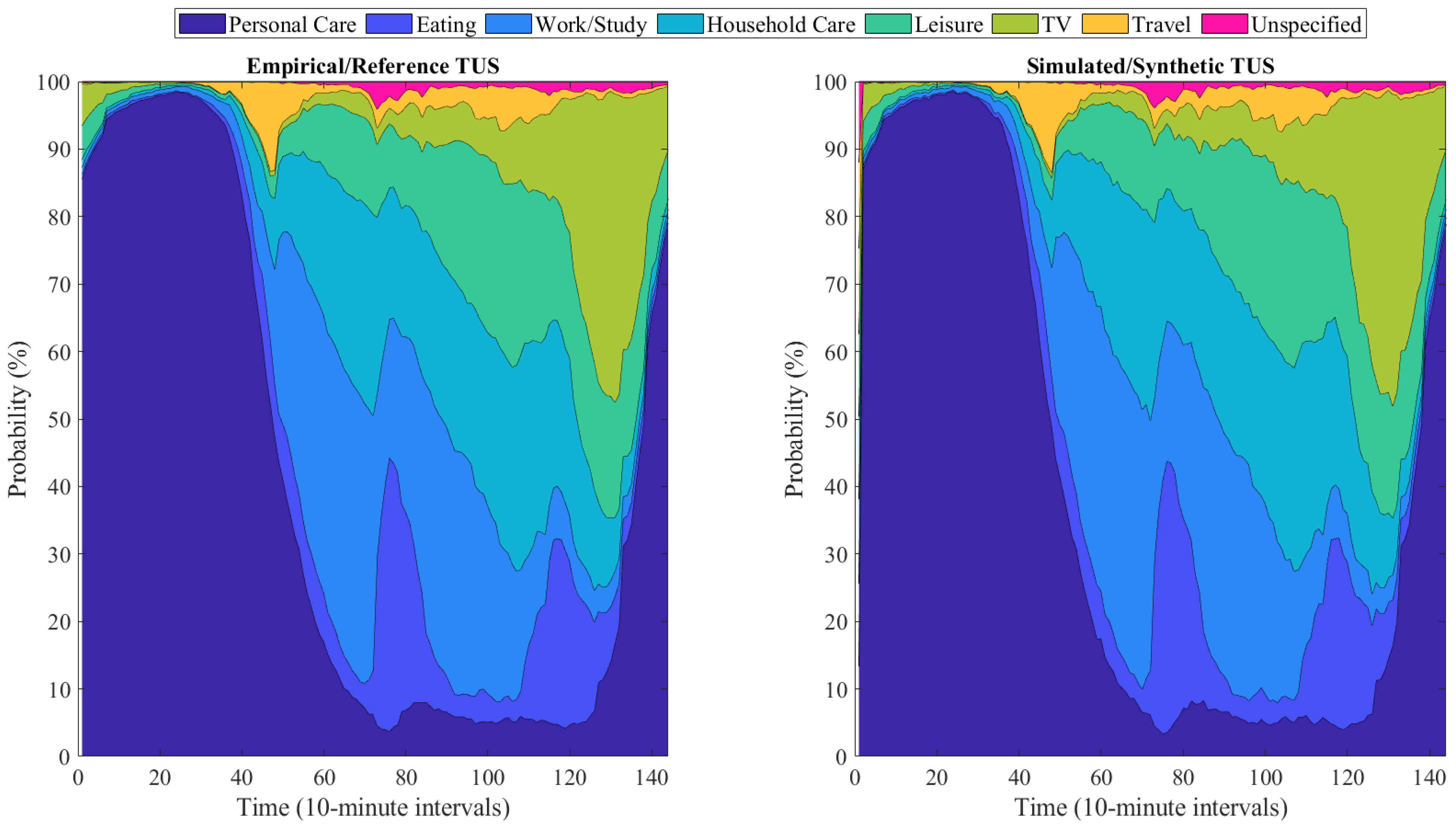
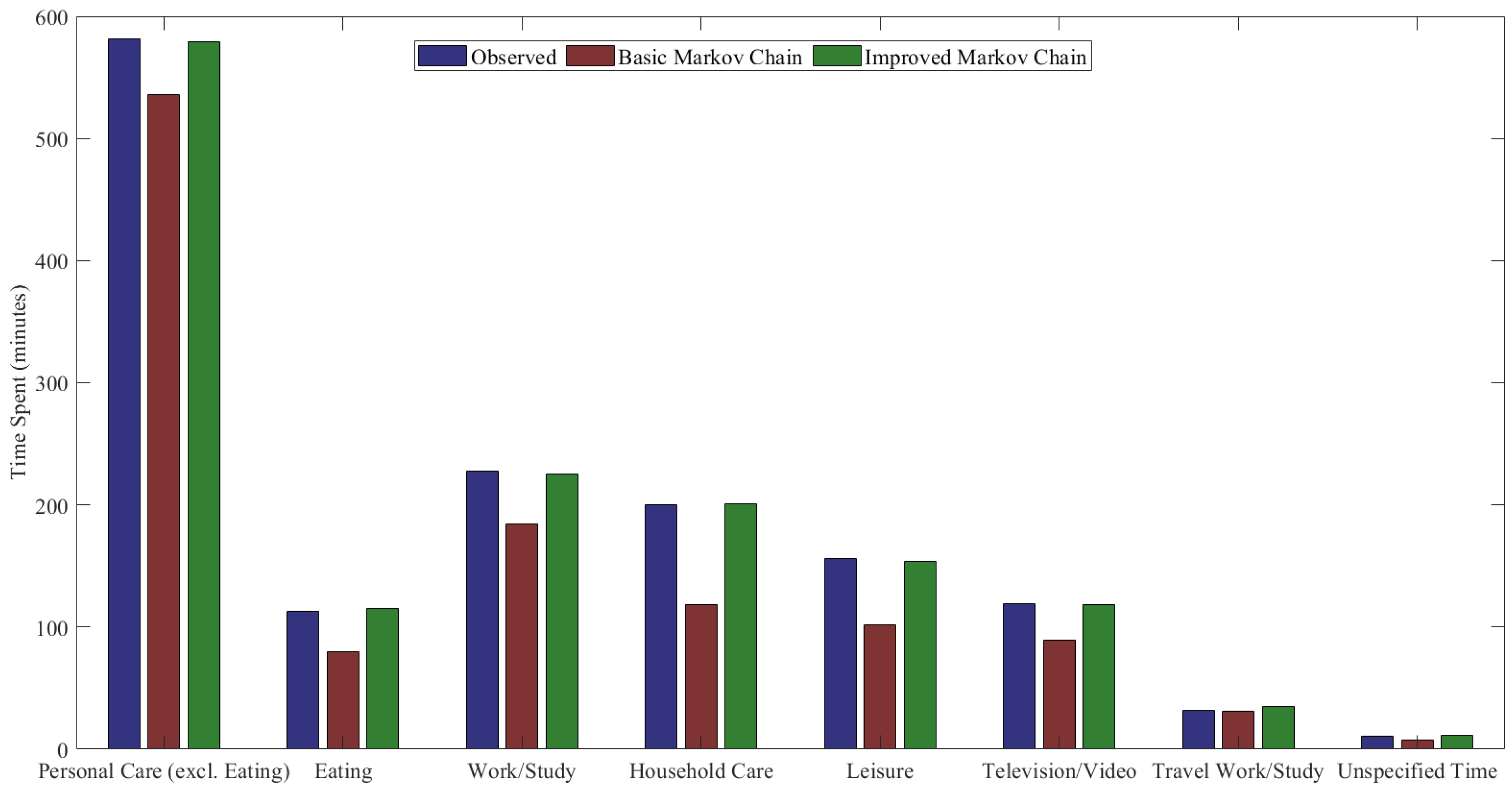
The model successfully reproduces empirical TUS activity patterns, with high agreement in activity durations and transitions (see further in Figure 2). The plots of probability distribution reveal that both the databases show an almost similar pattern and capture the transition from activity to activity at various times of the day. Personal care, including sleeping, dominates early hours and decreases as the day progresses. All work and study activities peak during the standard hours of the day, and leisure, watching TV, and household care all begin to peak later in the evening. Because of the much closer match between empirical data as well as synthetic data, it can be inferred that this model has well captured what is occurring. Comparison of times for different activities gave nearly consistent interpretation between the datasets. Most time was spent on personal care, averaging approximately 500 min in total spent per day, followed by work/study and household care. Importance was given to leisure, TV watching, and travel, which showed relatively shorter times but had a consistent profile over datasets. Minor variations were observed in most activities. Higher discrepancies were established for household care and leisure, which are due to inherent randomness in the simulation process. As shown in Table 4, the MSE values present some further evidence regarding the accuracy of simulating activities, like eating or unspecified activities, with very little deviation, MSE values near 0.
MSE values were a bit higher under household care and travel to work/study, showing some difficulty in simulation modeling for activities. Higher MSE in household care and leisure is expected due to their flexible and irregular nature. These activities vary significantly across household types and are often affected by personal preferences, making them more difficult to model precisely. However, error values at a low overall are a good indication of simulation in reproducing empirical patterns. In the end, as shown above, there is good correspondence between empirical and simulated data with respect to activity probabilities and durations. The reliability of the synthetic model is further reinforced by the low error rates, even though some minor discrepancies observed are identified for specific activities that warrant further improvement in future editions. Overall, the simulation achieves a high-level performance showing real-world activity trends and their durations. To quantify the benefit of our proposed framework, we compare our ‘Improved Markov Chain’ against a Basic Markov Chain baseline. This basic model is defined as a standard first-order Markov chain where transition probabilities are derived directly from empirical TUS frequencies using Equation (7), without the subsequent Bayesian calibration and constraint-based optimization layers. This baseline represents a common approach in the literature and serves to isolate the performance gains attributable to our dual-layer optimization method.
The comparison between the basic and improved Markov chain models highlights the improved model’s superior performance in replicating empirical activity patterns. Figure 3 illustrates a closer alignment between observed data and the improved model, particularly for activities like leisure, household care, and TV watching, where the basic model showed noticeable discrepancies. This visual improvement is supported by the MSE values in Table 4, where substantial reductions are evident: leisure decreases from 0.24 to 0.050, work/study from 0.50 to 0.011, and personal care from 0.91 to 0.038. The improved model exhibits enhanced accuracy in capturing activity transitions and time-use probabilities, effectively minimizing over- and underestimations observed in the basic model. The percentage improvements range from −87.78% (for eating, reflecting a minor discrepancy) to an impressive 97.8% for work/study, confirming the model’s robustness. While slight deviations persist due to inherent data variability, the improved model significantly enhances reliability across most activities.

4.2. Clustering

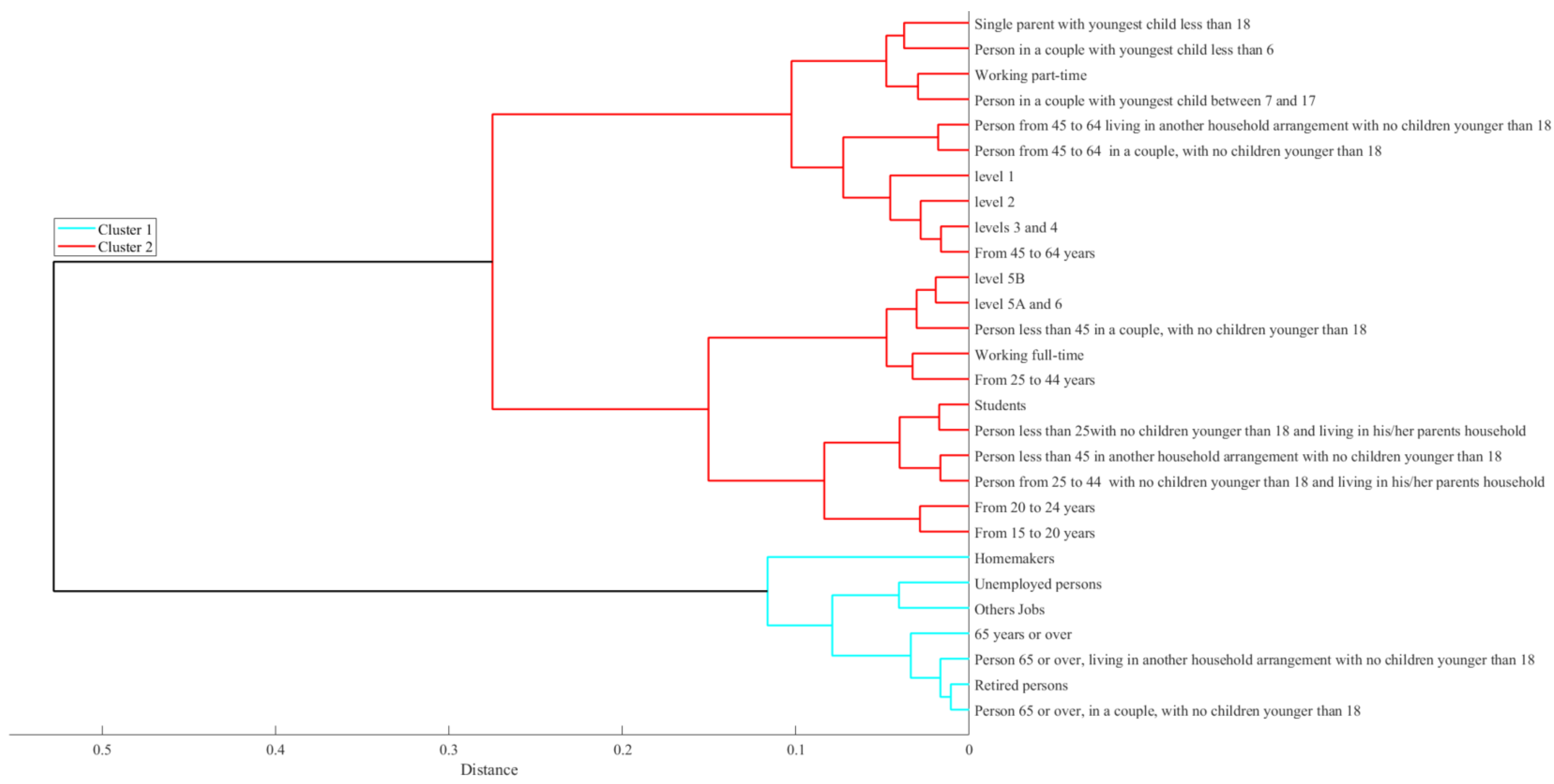
The aim of the clustering analysis is to differentiate demographic groups according to how individuals spend their time in various activities, such as personal care, eating, working, or studying, housework, leisure time, watching TV or movies, travel related to work or school, and other unspecified activities. We have used the silhouette method to determine the best number of clusters, which evaluates whether clusters can be established and remain consistent. The study ultimately pointed to two clusters as the best number, exposing strong differences in time use patterns between demographically differing people. The silhouette assessment indicates that k = 2 is the best configuration, since the two clusters have largely high scores, little overlap, and distinct separation between the two. Though, increased numbers of clusters (k = 3, k = 4, k = 5) would typically show greater overlap and less defined edges; all indicating poorer clustering.
Cluster 1 (See Table 5 and Figure 4) consists mostly of older adults, retirees, housewives, and unemployed individuals. They exhibit minimal or no work or academic obligations throughout the day. The time spent categories are as follows: Personal Care: They dedicate a large chunk of their day (580.86 min) to personal care. Household Tasks: They spend significant time on domestic duties (240.09 min). Leisure Activities: Recreational activities are a big part of their day, taking up 222.24 min. Watching TV/Videos: They also watch a lot of TV or videos, averaging 169.95 min daily. Work or Study: This group spends minimal time, just 30 min a day, on work or study, reflecting their lack of work or academic commitments. It is during life’s stage, or by the nature of employment, that these groups have customarily more flexible schedules and place importance on self-care and household maintenance and leisure. Cluster 2 includes young people, students, working people who do both full-time and part-time work, and those who take care of the family. The time-Use Patterns are: Higher allocation of time to work or study (231.41 min) and travel for work or study (31.38 min). Less time spent on household activities (153.98 min) and leisure activities (171.02 min) compared to cluster 1. Lower engagement in television/video consumption (113.64 min). These groups are primarily engaged in work or educational responsibilities and have tighter schedules, which reduces the time available for leisure and household maintenance. While the groups and clusters formed by using k-means and hierarchical methods are identical, they also support the compatibility of the two methods on this data. Time-use patterns of the two clusters have not altered much. Higher engagement in personal care, leisure activities, and household tasks is indicated in cluster 1, while cluster 2 spends more time on work/study and travel. While broad agreements exist in clustering results, the dendrogram allows for exploring groups and subgroups considering proximity. This will allow for further presentation of hierarchical relationships amongst cluster members not possible in k-means clustering.
The developed model allows family or household to be defined by sketching its members as different classes in the HUTUS data set, coupled with specific probability matrices defining activities separately for weekdays and weekends. These specific activity patterns are used to construct occupant profiles. The profiles can be aggregated for combined lighting demand, which shows how different behaviors interact dynamically with collective activities in the household. This study focuses on analyzing the impact of various household types on lighting power consumption and their potential for demand response strategies. The household types include single full-time working, single retired, couple full-time working, couple retired, and couple full-time working with two student children. Similar household archetypes have been commonly used in related studies in the literature.

4.3. Lighting Power Analysis

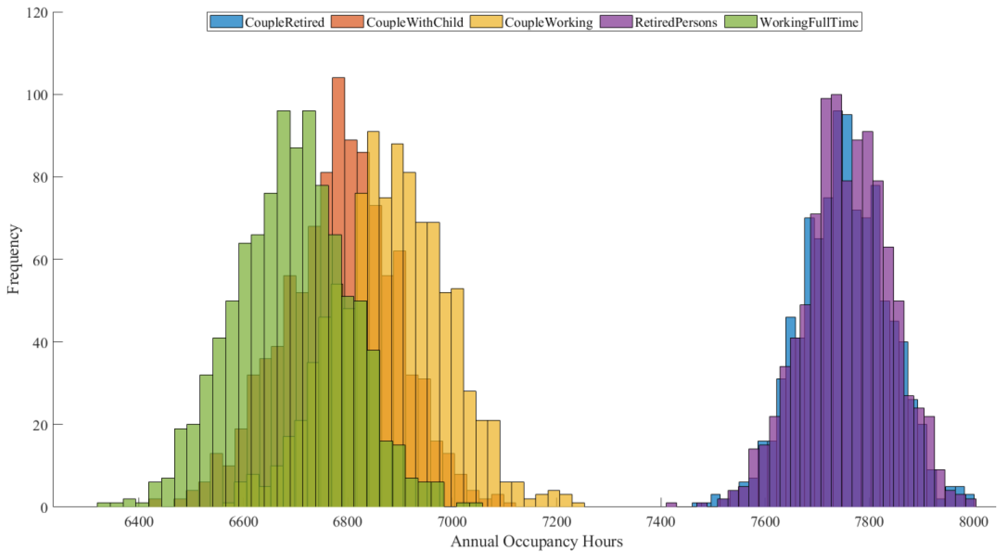
The results (see Figure 5 and Table 6) reveal two distinct clusters in the histogram: one around 7750–7800 h, representing “Retired Persons” and “Couple Retired”, and another around 6600–6900 h, representing “Working Full-Time”, “Couple with Child”, and “Couple Working”. The clear gap suggests that home presence is primarily driven by employment status rather than other lifestyle factors. This distinction aligns with expectations, as retired individuals spend significantly more time at home. The stochastic model captures this trend, reflecting the reduced home presence of employed individuals due to work or study commitments. Clustering analysis supports these findings, showing that retirees and older adults spend significantly more time at home, dedicating substantial time to personal care and household tasks. In contrast, working individuals and students allocate more time to work, study, and travel, reducing their home presence. Statistical measures reinforce this trend: “Couple Retired” averages 7752 h/year (IQR: 113 h), while “Retired Persons” average 7757 h/year (IQR: 113 h). The relatively low standard deviations (84 for both groups) indicate stable home presence.
“Couple with Child” and “Couple Working” exhibit distinct yet close occupancy patterns, averaging 6785 and 6884 h/year, respectively. While childcare responsibilities might suggest higher home occupancy for “Couple with Child”, the results indicate otherwise, likely due to structured childcare arrangements. The IQR for “Couple with Child” is 145 h, compared to 144 h for “Couple Working”, indicating a slightly broader spread in home time among working couples. Their standard deviations (109 vs. 110) suggest similar variability in occupancy patterns. The minimal difference between “Couple Retired” (7752 h, IQR: 113 h) and “Retired Persons” (7757 h, IQR: 113 h) suggests similar home presence patterns, likely influenced by social synchronization. The identical standard deviations (84) support the notion of a stable routine among retirees. Among working individuals, “Working Full-Time” averages 6692 h/year (IQR: 148 h), equating to 18.3 h/day at home. While a full-time job typically requires 8–9 h/day, this estimate might appear high unless remote work or long commutes are considered. The higher standard deviation (109) suggests greater variability, likely to be influenced by flexible work schedules. The distribution of home occupancy hours varies across household types. Working groups exhibit wider distributions (higher IQR values), reflecting variability due to overtime, travel, and social commitments. Retired groups show more concentrated patterns, consistent with stable routines. If the model does not explicitly account for out-of-home leisure activities, it may overestimate evening home occupancy. To improve accuracy, survey-based validation could help ensure stochastic profiles align with real-world time-use data.
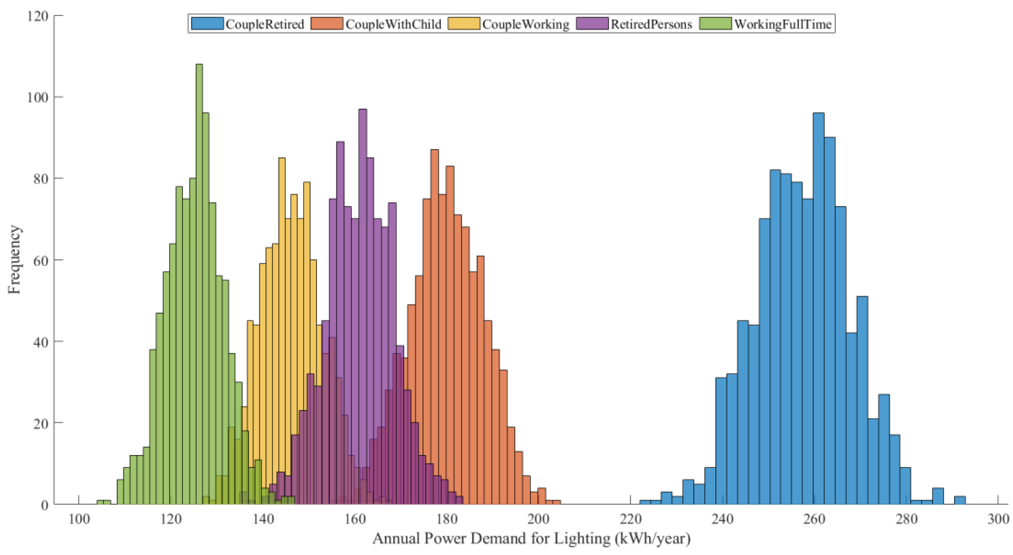
Extending the results, the histogram (see Figure 6) reflects distinct clusters for each household type in power consumption for lighting. The “Couple Retired” group exhibits the highest annual power demand (258 kWh), while “Working Full-Time” has the lowest (126 kWh). The separation between groups aligns with expected behavioral patterns: retired groups spend more time at home, leading to higher lighting demand, whereas working individuals have lower home occupancy, resulting in reduced demand. The occupancy-based modeling approach correctly differentiates between lifestyle-dependent lighting demand, confirming the validity of the stochastic approach. The shape of the distributions makes sense in terms of variability. Retired groups (“Couple Retired” & “Retired Persons”) have more concentrated distributions, meaning their demand is more stable. Working groups (“Couple Working” & “Working Full-Time”) show wider distributions, suggesting higher variability. Retired individuals follow routine home occupancy, whereas working individuals have varying schedules (overtime, flexible hours, commuting), leading to a broader spread. The statistical values further illustrate these points. For “Couple Retired”, the mean annual power demand is 258.21 kWh with a standard deviation of 10.96 kWh, indicating a stable demand. “Couple With Child” has a mean of 180.20 kWh and a standard deviation of 8.03 kWh, while “Couple Working” has a mean of 146.60 kWh and a standard deviation of 7.41 kWh. “Retired Persons” show a mean of 160.96 kWh with a standard deviation of 7.63 kWh, and “Working Full-Time” has the lowest mean demand at 125.53 kWh with a standard deviation of 6.63 kWh. These values highlight the variability in power demand across different household types. The power demand range is reasonable compared to expected lighting needs. A 258 kWh/year demand for retired households translates to about 29 W continuously used for 8760 h, which is realistic given evening lighting usage. A 126 kWh/year demand for full-time workers suggests much lower use (~14 W continuously), which aligns with reduced home presence.
Table 7 confirms that retired groups have the highest and most stable lighting demand, while working households show lower and more variable consumption. “Couple Retired” has the highest mean (258.21 kWh) with a low IQR (14.14 kWh), indicating consistent use. “Retired Persons” follow a similar trend (160.96 kWh, IQR 10.46 kWh). In contrast, working households have lower means and wider variability. “Couple Working” (146.60 kWh, IQR 9.95 kWh) and “Working Full-Time” (125.53 kWh, IQR 9.05 kWh) show greater fluctuations due to irregular schedules and reduced home presence. “Couple With Child” (180.20 kWh, IQR 11.11 kWh) falls in between, influenced by childcare routines.
Minimum and maximum values further highlight stability differences. Retired households exceed 250 kWh, while working groups rarely go beyond 150–180 kWh, reinforcing the model’s accuracy in reflecting real-world household behavior. For Luxembourg, based on EU data, the average household consumed 154 kWh of electricity for lighting over a year in 2022. In 2020, the average electricity consumption per household in Luxembourg was 3586 kWh. Given that lighting typically accounts for 8% to 10% of household electricity use, this translates to approximately 358 kWh. This data supports the model’s estimates, validating the reasonableness of the power demand range for different household types. The developed stochastic model for household lighting power demand demonstrates a logical and structured validation approach, ensuring robust assessment of energy consumption patterns. The unit conversions from kWh to GWh are accurately handled, allowing meaningful comparisons with real-world benchmarks. By integrating household distribution shares, the model effectively represents variations across different household types. Validation against EU residential lighting demand standards shows a minor deviation of +3.42%, confirming that the model closely aligns with empirical data. This small overestimation suggests that the model reliably captures household lighting behavior, making it a credible tool for energy analysis and policy planning.

4.4. Energy Efficiency Strategies

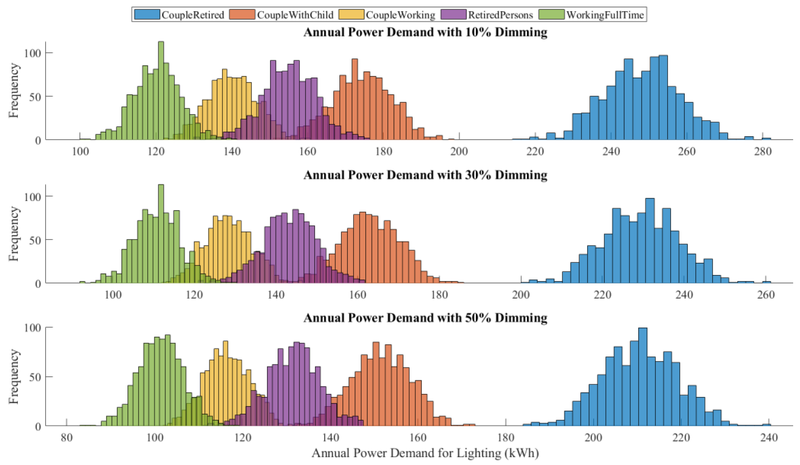
As dimming increases from 10% to 50%, the peak values of the histograms shift leftward, indicating a clear reduction in overall lighting energy demand (see Figure 7). This shift occurs because the dimming strategy reduces power consumption during activities like leisure and television viewing, which are frequent, leading to a notable impact on annual consumption. The demand reduction is non-linear, with a greater relative impact at higher dimming levels. For example, “Couple Retired” has a mean annual lighting demand of 248.79 kWh at 10% dimming, which decreases to 229.96 kWh at 30% dimming and 211.13 kWh at 50% dimming, corresponding to reductions of 3.65%, 10.94%, and 18.23%, respectively. Different household groups exhibit varying distributions in annual power demand. “Working Full-Time” has the lowest mean demand, starting at 120.77 kWh at 10% dimming and reducing to 101.75 kWh at 50% dimming (reductions of 3.79% and 18.94%), while “Retired Persons” has a higher mean demand, decreasing from 155.09 kWh to 131.63 kWh, showing reductions of 3.64% to 18.22%. These differences reflect household composition and daily routines, where working households rely more on artificial lighting during later evening hours, while retired households utilize more daylight, reducing their artificial lighting needs.
The spread of lighting demand, as reflected in standard deviation (StdDev) and interquartile range (IQR), also differs across groups. For “Couple Working”, the standard deviation decreases from 7.03 kWh at 10% dimming to 5.77 kWh at 50% dimming, indicating a more uniform reduction as dimming levels increase. Similarly, “Couple with Child” exhibits a narrowing demand range, with minimum values reducing from 149.36 kWh to 132.84 kWh, while maximum values drop from 198.24 kWh to 173.34 kWh at 50% dimming. Despite these reductions, maximum demand values remain relatively high, as some households have longer leisure/TV time, leading to less pronounced dimming effects. The non-linear reduction is due to the unequal distribution of dimmable activities, where dimming is only applied to two activity states and does not fully represent household lighting demand. Overlap in minimum values suggests partial dimming effectiveness, with some homes already exhibiting low baseline lighting demand. For example, “Couple with Child” shows a mean reduction from 174.51 kWh at 10% dimming to 151.71 kWh at 50% dimming, corresponding to reductions of 3.16%, 9.49%, and 15.81%. Similarly, “Couple Working” starts at 140.63 kWh and reduces to 116.73 kWh, with reductions of 4.08%, 12.23%, and 20.38%. The “Working Full-Time” group remains on the higher end of the scale, with mean values ranging from 120.77 kWh at 10% dimming to 101.75 kWh at 50% dimming, suggesting that automated dimming or occupancy-based lighting control might be more effective for them. Overall, the “Retired Persons” group shows a larger relative reduction in demand, suggesting they spend more time in dimmable activities. Some groups, such as “Couple Retired” and “Couple with Child”, have similar lighting demand profiles, indicating that dimming policies could be more effective when customized based on activity type rather than household composition. The higher standard deviations in working groups suggest greater variability in occupant behavior, making flexible dimming strategies crucial for optimizing energy savings. Higher participation rates significantly reduce total lighting demand, with variations across household types (see Figure 8).
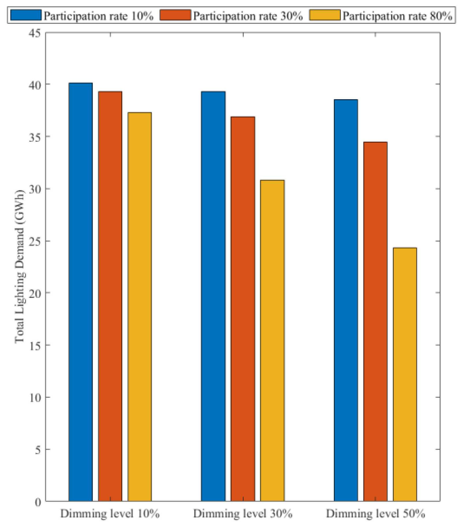
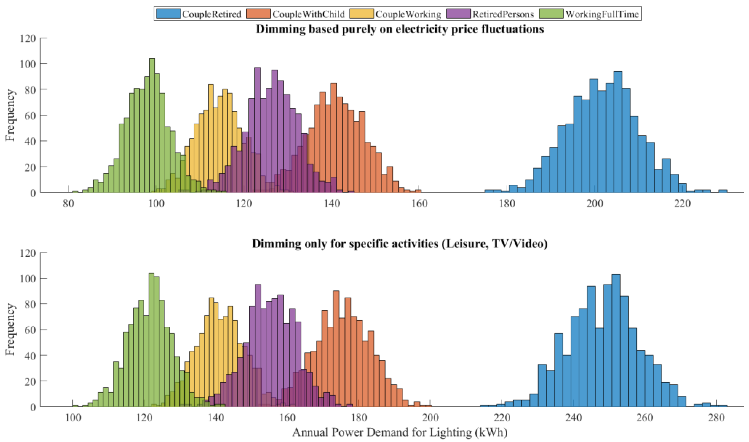
“Working Full-Time” (28.4%) and “Couple with Child” (26.4%) contribute the most to total demand, while “Couple Retired” (9.1%) has the lowest impact due to lower home presence. At 10% dimming, increasing participation from 10% to 80% lowers demand from 40.14 GWh to 37.30 GWh, showing modest savings. At 30% dimming, demand drops from 39.32 GWh to 30.79 GWh, showing greater efficiency as more homes participate. The largest reduction occurs at 50% dimming, where demand falls from 38.54 GWh to 24.34 GWh, confirming that higher dimming levels maximize savings. However, diminishing returns emerge beyond 30% dimming, meaning additional participation has less impact at higher reductions. Households with irregular schedules, like “Working Full-Time”, may benefit more from automated strategies, while retired groups respond better to voluntary participation. These findings highlight the importance of tailored participation incentives and policy interventions to optimize savings across different household types. The analysis of lighting demand under different dimming strategies compares two approaches: dimming based on electricity price fluctuations and dimming for specific activities such as leisure and TV/video (see Figure 9). Dimming based on electricity price fluctuations achieves the highest reduction in power demand, with an average decrease of approximately 21.6% across all household types compared to no dimming. For example, the “Couple Retired” group sees a reduction from 257.50 kWh to 201.84 kWh (21.61%), while the “Working Full-Time” group experiences a decrease from 125.22 kWh to 98.07 kWh (21.68%). This method is most effective because it dynamically adjusts lighting use based on cost changes, affecting all activities. In contrast, dimming only for leisure and TV/video activities has a much smaller impact, reducing demand by only around 3% across most groups. For instance, the “Couple Retired” group’s demand decreases to 248.29 kWh (3.58%), and the “Working Full-Time” group’s demand drops to 121.51 kWh (2.96%). The limited savings are due to dimming, affecting only specific activities, leaving other high-consumption activities unchanged. Overall, price-based dimming is significantly more effective than activity-based dimming, as it covers all household activities rather than just selecting ones. Households with higher lighting demand, such as retirees, benefit more from price-based dimming because they spend more time at home.
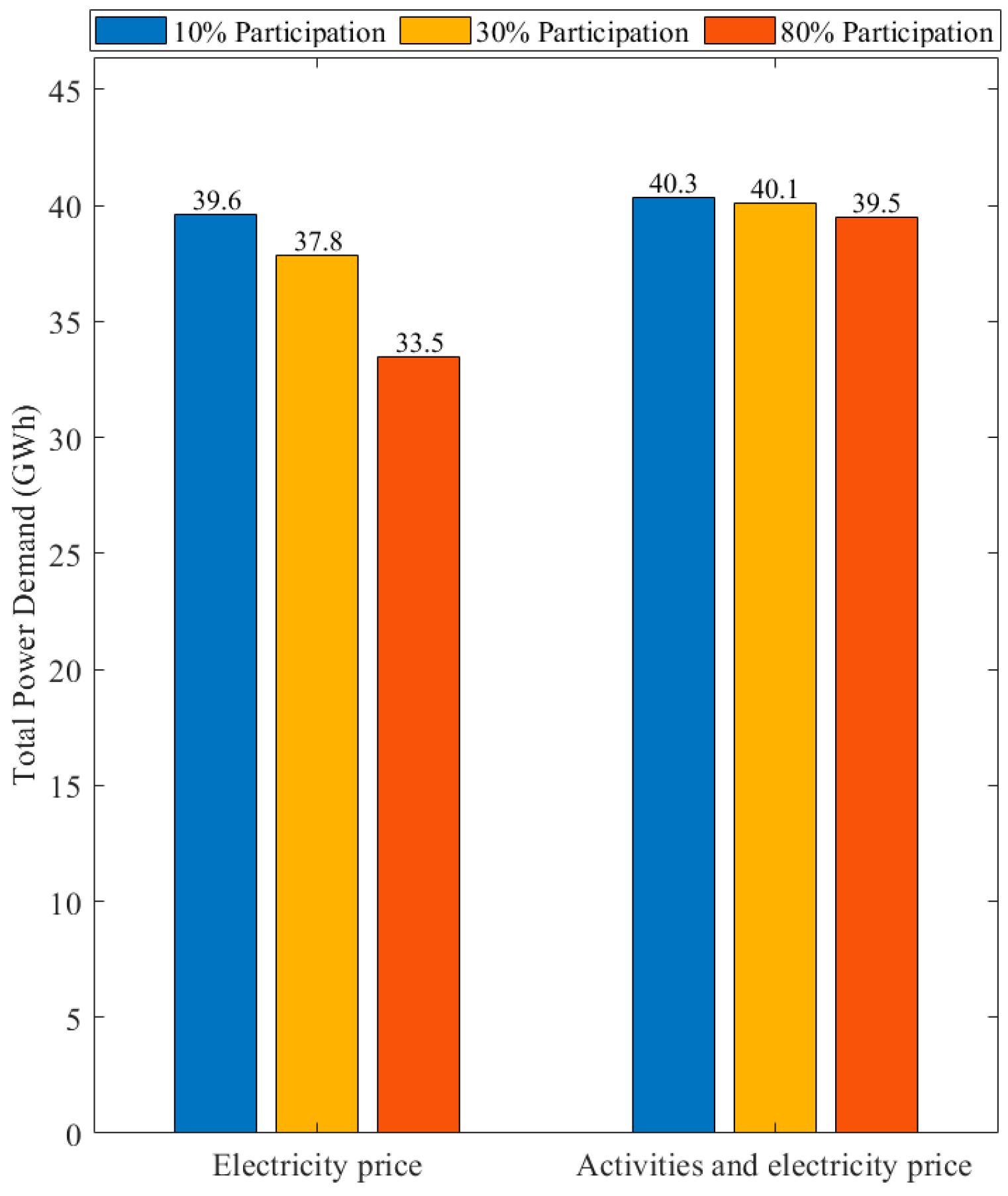
Working households show smaller reductions, as they already have lower lighting use due to time spent outside. These results highlight that dynamic pricing-based dimming strategies are more effective than fixed activity-based dimming for reducing residential lighting demand. The analysis of the effect of participation rate on total lighting demand compares two dimming strategies (price-based and activity-based dimming) under different participation rates (10%, 30%, and 80%). The results highlight the varying effectiveness of each method in reducing total lighting demand (GWh) (see Figure 10).
Dimming based on electricity price fluctuations achieves a significant reduction in demand, with higher participation leading to greater savings. The baseline demand is 40.47 GWh, which decreases to 39.59 GWh (10% participation), 37.84 GWh (30%), and 33.46 GWh (80%). The reduction is progressive and substantial, confirming that dynamic price-driven dimming is an effective strategy for managing household lighting consumption. In contrast, dimming only during specific activities (Leisure, TV/Video) results in minimal reductions. The baseline demand remains nearly unchanged, reducing only from 40.47 GWh to 40.34 GWh (10%), 40.09 GWh (30%), and 39.47 GWh (80%). This limited effect suggests that targeting only a subset of household activities does not fully optimize savings. Price-based dimming is far more effective than activity-based dimming, as it impacts all household lighting use rather than specific activities. Even at 80% participation, activity-based dimming achieves only a 2.47% reduction, whereas price-based dimming reduces demand by 17.34%. Encouraging higher participation rates is crucial, but the type of dimming strategy plays a more significant role in determining energy savings. These findings suggest that policy measures should focus on price-based dimming strategies to maximize household lighting efficiency while promoting participation.

5. Discussion

This study develops a stochastic framework for modeling occupant behavior and lighting demand in Luxembourg’s residential sector. It integrates empirical HETUS data with an enhanced Markov chain model, using Bayesian calibration and constraint-based optimization to improve transition accuracy and behavioral realism. This study develops a stochastic framework for modeling occupant behavior and lighting demand in Luxembourg’s residential sector, aligning with LetzPower’s goal of consumer-driven energy optimization through data-driven insights and efficiency strategies [13]. Unlike prior studies [33,39], it explicitly links occupant activity to lighting power demand and evaluates dimming strategies for energy savings. Such validated, high-resolution occupant profiles are crucial inputs for advanced control strategies like Model Predictive Control (MPC), where predicting future loads is essential for optimizing building energy performance.
A key methodological innovation is the dual-layer optimization approach, which enhances the realism and accuracy of occupant profiles by calibrating transition probabilities and enforcing behavioural constraints. Bayesian updating with Dirichlet priors aligns transition probabilities with observed data, while constraint-based optimization ensures empirical plausibility by correcting unrealistic activity patterns. This approach enforces realistic sleep durations and work hours, minimizing deviations from calibrated TPMs. The iterative adjustment algorithm fine-tunes activity sequences efficiently, reducing computational costs. These refinements enhance the model’s ability to generate accurate occupant-driven lighting demand profiles, improving its application for energy demand simulations and demand response analysis.
The clustering analysis differentiates demographic groups based on time-use patterns using the silhouette method, identifying K = 2 as optimal due to minimal intra-cluster variation and distinct group separation. Cluster 1 (older adults, retirees, homemakers, unemployed) spends more time on personal care and leisure, while Cluster 2 (working individuals, students) allocates more time to work/study and travel. Both k-means and hierarchical methods yield consistent results, confirming the robustness of classification. These clusters provide critical insights into household lighting demand and demand response strategies. Cluster 1 households exhibit higher artificial lighting use, as occupants remain home for longer periods, whereas Cluster 2 relies more on natural daylight due to structured work schedules. The ability to differentiate occupant groups enhances energy consumption modeling accuracy, enabling more effective demand-side management strategies tailored to specific household types.
Section 4.3 and Section 4.4 present the results of lighting power analysis and energy efficiency strategies, respectively. Annual home occupancy analysis reveals that retired individuals spend significantly more time at home, leading to higher lighting power consumption (258 kWh for Couple Retired, compared to 126 kWh for Working Full-Time). The stochastic model effectively captures home presence variability, demonstrating its influence on energy demand. Dimming strategies significantly reduce lighting energy consumption, with price-based dimming achieving a 21.6% demand reduction, outperforming activity-based dimming, which is limited to leisure-related activities. Price-based dimming impacts all activities, leading to greater overall reductions. In this study, price-based dimming is assumed to be an automated response to dynamic electricity price signals, adjusting lighting power in real-time based on cost variations. This approach ensures that households optimize their lighting consumption without manual intervention, maximizing energy savings. The analysis further shows that higher participation rates in dimming programs enhance savings, though the type of dimming strategy remains the dominant factor.
These findings highlight the potential of demand-side management strategies to optimize residential lighting consumption and inform future energy efficiency policies. Home-based individuals, such as retirees and homemakers, should be prioritized for dimming-based demand response programs, as they have higher lighting consumption and greater flexibility in adjusting usage patterns. In contrast, working individuals and students would benefit more from automated lighting control systems that optimize energy use during occupied hours. To further enhance energy efficiency in residential buildings, policymakers should mandate smart lighting systems in new constructions, particularly for households with predictable occupancy patterns. Additionally, retrofitting subsidies and financial incentives should be introduced to encourage the adoption of dimmable and sensor-based lighting systems in existing homes, ensuring cost-effective energy savings. Public awareness programs and behavioral nudges could further drive adoption, reinforcing the role of occupant behavior in optimizing energy efficiency.
While this model was specifically calibrated for Luxembourg, the framework is generalizable. The use of the Harmonized European Time Use Surveys (HETUS) as a data source means the methodology could be readily applied to other EU member states, provided local census data is used to define household archetypes. However, the specific quantitative results (e.g., kWh demand) are context-dependent and would vary with local climate (affecting daylight), building stock, and cultural time-use patterns.

Limitations

Several limitations of this study stem from the reliance on HETUS data and methodological simplifications. This study specifically focuses on lighting demand, excluding other household energy uses such as heating, cooling, and appliance consumption. Future work will address this limitation by extending the approach to include these high-consumption appliances and evaluating whole-home energy demand. Additionally, the focus on eight major activities excludes minor but energy-intensive behaviors, such as brief high-power tasks (e.g., boiling water, reheating food, or charging electronic devices), which could contribute to short-term peak demand. Several sources of uncertainty should be acknowledged. First, the HETUS data, while comprehensive, is based on self-reported diaries, which may contain reporting biases. Second, uncertainty exists in the physical parameters of the lighting model, such as the assumed lighting technology mix and lux thresholds, which can vary significantly between households. Finally, the stochastic nature of the model itself means that any single generated profile is one realization of a probabilistic process; therefore, conclusions are drawn from aggregated results over many simulations.
A further limitation is the choice of an enhanced Markov chain over other advanced techniques. While methods like Hidden Markov Models (HMMs) and Agent-Based Models (ABMs) can offer a richer state representation or simulate complex agent interactions, they often require more extensive data and entail a significantly higher computational burden. Our dual-layer optimization approach was chosen as a practical and scalable solution that provides a robust balance between behavioral realism and computational efficiency for this study’s scope.
Furthermore, our lighting activation rule, while based on common modeling practices, simplifies behavior by excluding lighting use during other potential activities, which could be a focus for future refinement.

6. Conclusions

This study developed a stochastic framework for modeling occupant behavior and lighting energy demand in residential buildings, focusing on Luxembourg. Using HETUS data, Markov chains, and dual-layer optimization approach, the framework minimized assumptions, providing realistic occupant profiles and energy demand simulations. The study revealed several key insights:
  • The study introduces a novel dual-layer optimization approach, combining Bayesian updating with Dirichlet priors for transition probability calibration and constraint-based optimization to enhance the realism of occupant profiles. This approach improves data alignment with observed Time Use Survey (TUS) patterns and behavioral realism. The model demonstrates a minor deviation of +3.42% when validated against EU residential lighting demand standards
  • Household types significantly influence energy consumption. The study found that “Couple Retired” groups exhibit the highest annual power demand at 258 kWh, while “Working Full-Time” groups show the lowest at 126 kWh. This is largely due to the differences in time spent at home and the presence of work or study obligations.
  • Increased participation in dimming programs leads to greater savings. However, the study also emphasizes that the type of dimming strategy (price-based vs. activity-based) has a greater influence on energy savings than the participation rate
This work advances occupant-centric energy modeling by providing insights into energy-saving behaviors and their influence on lighting demand. The findings lay a foundation for tailored energy policies and sustainable building design strategies, highlighting the critical role of occupant behavior in achieving energy efficiency goals. In future studies, the model’s application will be expanded to include equipment usage, thermal load analysis, Power to Heat, the evolving role of occupants as both consumers and prosumers and considering the integration of electric vehicle usage.

Supplementary Materials

The following supporting information can be downloaded at: https://www.mdpi.com/article/10.3390/en18195133/s1, Table S1: Detailed activity taxonomy for time use classification; Table S2: High-level categorization framework for activity clustering in time use analysis.

Author Contributions

V.A. and R.F.; methodology, V.A. and R.F.; validation, V.A.; investigation, V.A.; data curation, V.A.; writing—original draft preparation, V.A.; writing—review and editing, R.F.; visualization, V.A.; supervision, R.F.; funding acquisition, R.F. All authors have read and agreed to the published version of the manuscript.

Funding

This research was supported by the Luxembourg National Research Fund (FNR) and PayPal (PEARL grant 13342933/Gilbert Fridgen) and by the Fondation Enovos in the frame of the “LetzPower” research project.

Data Availability Statement

Data is contained within the article or Supplementary Material.

Conflicts of Interest

The authors declare no conflicts of interest.

Abbreviations

Nomenclature
Greek Symbols Subscript
τ ω Transmittance of the window i Current state/activity
θ Z Solar zenith angle j Transition state/activity
δ Solar declination k Time step
ψ Penalty functionAcronym
µ i j Prior parameter for the transition from i to jABMAgent-Based Modelling
Latin Symbols ACLActivity Coding List
E T i Expected time spent in activity iATUSAmerican Time Use Survey
E d i f f u s e Diffuse illuminanceDSMDemand-Side Management
E d i r e c t Direct illuminanceDRDemand Response
F Fitness functionEEOSEnergy Efficiency Obligation Scheme
F b Illuminance coefficient for direct radiation W/m2GAGenetic Algorithm
F d Illuminance coefficient for diffuse radiation W/m2HETUSHarmonized European Time Use Surveys
G d i f f u s e Diffuse horizontal radiation W/m2HMMHidden Markov Models
G d i r e c t Direct normal radiation W/m2HVACHeating, ventilation, and air conditioning
L Total daylight illuminanceIQRInterquartile Range
L o i Lower bound from HETUS datanZEBNet-Zero Energy Buildings
U P i Upper bound from HETUS dataPDFProbability Density Function
N Number of states/activitiesMSEMean Square Error
P i j k Probability of transitioning from state i to state j at time step kSGSCSmart Grid Smart City
S k Current state at time step kTPMTransition Probability Matrix
T i t a r g e t Target time for activity i TSTime Spent on activities
Y i Empirical/reference state TUSTime Use Survey
d i Total time spent in activityWCSSWithin Cluster Sum of Squares
a i Average intra-cluster distance
b i Average distance from a data point i

References

  1. World Green Building Council. Bringing Embodied Carbon Upfront: Coordinated Action for the Building and Construction Sector to Tackle Embodied Carbon; World Green Building Council: Toronto, ON, Canada; London, UK, 2019; Available online: https://www.worldgbc.org/ (accessed on 1 January 2025).
  2. Levine, D.Ü.-V.M.; Blok, K.; Geng, L.; Harvey, D.; Lang, S.; Levermore, G.; Mehlwana, A.M.; Mirasgedis, S.; Novikova, A.; Rilling, J.; et al. (Eds.) Residential and Commercial Buildings; Cambridge University Press: Cambridge, UK; New York, NY, USA, 2007. [Google Scholar]
  3. Luxembourg’s Integrated National Energy and Climate Plan for 2021–2030. 2020. Available online: https://energy.ec.europa.eu/system/files/2020-07/lu_final_necp_main_en_0.pdf (accessed on 1 December 2024).
  4. European Commission. 2050 Long-Term Strategy. Available online: https://climate.ec.europa.eu/eu-action/climate-strategies-targets/2050-long-term-strategy_en (accessed on 1 March 2025).
  5. European Union Eurostat. Harmonised European Time Use Surveys (HETUS): 2018 Guidelines (Re-Edition); Eurostat: Luxembourg, 2020; Available online: https://ec.europa.eu/eurostat (accessed on 1 December 2024).
  6. Long-Term Renovation Strategy for Luxembourg. 2020. Available online: https://energy.ec.europa.eu/system/files/2020-09/lu_2020_ltrs_official_en_translation_0.pdf (accessed on 1 December 2024).
  7. Frank, R. Review and Growth Prospects of Renewable Energy in Luxembourg: Towards a Carbon-Neutral Future. In Proceedings of the 4th International Conference on Smart Grid and Renewable Energy, Doha, Qatar, 8–10 January 2024. Available online: https://ieeexplore.ieee.org/document/10428765 (accessed on 1 December 2024).
  8. Arabzadeh, V.; Frank, R. Creating a renewable energy-powered energy system: Extreme scenarios and novel solutions for large-scale renewable power integration. Appl. Energy 2024, 374, 124088. [Google Scholar] [CrossRef]
  9. The Luxembourg Government. Luxembourg’s Integrated National Energy and Climate Plan for the Period 2021–2030 (PNEC). Available online: https://gouvernement.lu/en/dossiers/2023/2023-pnec.html (accessed on 1 November 2024).
  10. Ville de Luxembourg (VDL). Luxembourg City Facts and Figures. Available online: https://www.vdl.lu/en/city/a-glance/facts-and-figures (accessed on 1 September 2024).
  11. Osman, M.; Ouf, M. A comprehensive review of time use surveys in modelling occupant presence and behavior: Data, methods, and applications. Build. Environ. 2021, 196, 107785. [Google Scholar] [CrossRef]
  12. Osman, M.; Saad, M.M.; Ouf, M.; Eicker, U. From buildings to cities: How household demographics shape demand response and energy consumption. Appl. Energy 2024, 356, 122359. [Google Scholar] [CrossRef]
  13. LetzPower! Interdisciplinary Centre for Security, and Trust (SnT). Power System Information Transparency for Households in Lëtzebuerg. Available online: https://www.uni.lu/snt-en/research-projects/letzpower/ (accessed on 4 January 2025).
  14. Andolfi, L.; Baima, R.L.; Burcheri, L.M.; Pavić, I.; Fridgen, G. Sociotechnical design of building energy management systems in the public sector: Five design principles. Appl. Energy 2025, 377, 124628. [Google Scholar] [CrossRef]
  15. Fernández, J.D.; Menci, S.P.; Lee, C.M.; Rieger, A.; Fridgen, G. Privacy-preserving federated learning for residential short-term load forecasting. Appl. Energy 2022, 326, 119915. [Google Scholar] [CrossRef]
  16. Körner, M.-F.; Sedlmeir, J.; Weibelzahl, M.; Fridgen, G.; Heine, M.; Neumann, C. Systemic risks in electricity systems: A perspective on the potential of digital technologies. Energy Policy 2022, 164, 112901. [Google Scholar] [CrossRef]
  17. Zhou, X.; Mei, Y.; Liang, L.; Mo, H.; Yan, J.; Pan, D. Modeling of occupant energy consumption behavior based on human dynamics theory: A case study of a government office building. J. Build. Eng. 2022, 58, 104983. [Google Scholar] [CrossRef]
  18. Luo, M.; Zheng, Q.; Zhao, Y.; Zhao, F.; Zhou, X. Developing occupant-centric smart home thermostats with energy-saving and comfort-improving goals. Energy Build. 2023, 299, 113579. [Google Scholar] [CrossRef]
  19. Kaspar, K.; Nweye, K.; Buscemi, G.; Capozzoli, A.; Nagy, Z.; Pinto, G.; Eicker, U.; Ouf, M.M. Effects of occupant thermostat preferences and override behavior on residential demand response in CityLearn. Energy Build. 2024, 324, 114830. [Google Scholar] [CrossRef]
  20. Pereira, P.F.; Ramos, N.M.M.; Almeida, R.M.S.F.; Simões, M.L. Methodology for detection of occupant actions in residential buildings using indoor environment monitoring systems. Build. Environ. 2018, 146, 107–118. [Google Scholar] [CrossRef]
  21. Jones, R.V.; Fuertes, A.; Gregori, E.; Giretti, A. Stochastic behavioural models of occupants’ main bedroom window operation for UK residential buildings. Build. Environ. 2017, 118, 144–158. [Google Scholar] [CrossRef]
  22. Andersen, R.; Fabi, V.; Toftum, J.; Corgnati, S.P.; Olesen, B.W. Window opening behaviour modelled from measurements in Danish dwellings. Build. Environ. 2013, 69, 101–113. [Google Scholar] [CrossRef]
  23. Carmenate, T.; Inyim, P.; Pachekar, N.; Chauhan, G.; Bobadilla, L.; Batouli, M.; Mostafavi, A. Modeling Occupant-Building-Appliance Interaction for Energy Waste Analysis. Procedia Eng. 2016, 145, 42–49. [Google Scholar] [CrossRef]
  24. Rafsanjani, H.N.; Ghahramani, A. Towards utilizing internet of things (IoT) devices for understanding individual occupants’ energy usage of personal and shared appliances in office buildings. J. Build. Eng. 2020, 27, 100948. [Google Scholar] [CrossRef]
  25. Laaroussi, Y.; Bahrar, M.; El Mankibi, M.; Draoui, A.; Si-Larbi, A. Occupant presence and behavior: A major issue for building energy performance simulation and assessment. Sustain. Cities Soc. 2020, 63, 102420. [Google Scholar] [CrossRef]
  26. Su, S.; Li, G.; Ding, Y.; Sun, A.; Xu, M. A dynamic simulation model for building cooling and heating energy considering climate-building system-occupant interactions. Case Stud. Therm. Eng. 2024, 61, 105145. [Google Scholar] [CrossRef]
  27. Tsang, T.-W.; Wong, L.-T.; Lung, H.-T.; Mui, K.-W. Stochastic behavioral models of bedroom window operation in sub-tropical residential buildings. Build. Environ. 2024, 262, 111784. [Google Scholar] [CrossRef]
  28. Virote, J.; Neves-Silva, R. Stochastic models for building energy prediction based on occupant behavior assessment. Energy Build. 2012, 53, 183–193. [Google Scholar] [CrossRef]
  29. Fabi, V.; Andersen, R.K.; Corgnati, S. Verification of stochastic behavioural models of occupants’ interactions with windows in residential buildings. Build. Environ. 2015, 94, 371–383. [Google Scholar] [CrossRef]
  30. Carlucci, S.; Causone, F.; Biandrate, S.; Ferrando, M.; Moazami, A.; Erba, S. On the impact of stochastic modeling of occupant behavior on the energy use of office buildings. Energy Build. 2021, 246, 111049. [Google Scholar] [CrossRef]
  31. Yun, G.Y.; Tuohy, P.; Steemers, K. Thermal performance of a naturally ventilated building using a combined algorithm of probabilistic occupant behaviour and deterministic heat and mass balance models. Energy Build. 2009, 41, 489–499. [Google Scholar] [CrossRef]
  32. Mylonas, A.; Tsangrassoulis, A.; Pascual, J. Modelling occupant behaviour in residential buildings: A systematic literature review. Build. Environ. 2024, 265, 111959. [Google Scholar] [CrossRef]
  33. Osman, M.; Ouf, M.; Azar, E.; Dong, B. Stochastic bottom-up load profile generator for Canadian households’ electricity demand. Build. Environ. 2023, 241, 110490. [Google Scholar] [CrossRef]
  34. Mosteiro-Romero, M.; Quintana, M.; Stouffs, R.; Miller, C. A data-driven agent-based model of occupants’ thermal comfort behaviors for the planning of district-scale flexible work arrangements. Build. Environ. 2024, 257, 111479. [Google Scholar] [CrossRef]
  35. McKenna, E.; Krawczynski, M.; Thomson, M. Four-state domestic building occupancy model for energy demand simulations. Energy Build. 2015, 96, 30–39. [Google Scholar] [CrossRef]
  36. Jang, H.; Kang, J. A stochastic model of integrating occupant behaviour into energy simulation with respect to actual energy consumption in high-rise apartment buildings. Energy Build. 2016, 121, 205–216. [Google Scholar] [CrossRef]
  37. Chen, J.; Adhikari, R.; Wilson, E.; Robertson, J.; Fontanini, A.; Polly, B.; Olawale, O. Stochastic simulation of occupant-driven energy use in a bottom-up residential building stock model. Appl. Energy 2022, 325, 119890. [Google Scholar] [CrossRef]
  38. Wolf, S.; Calì, D.; Alonso, M.J.; Li, R.; Andersen, R.K.; Krogstie, J.; Madsen, H. Room-level occupancy simulation model for private households. J. Phys. Conf. Ser. 2019, 1343, 012126. [Google Scholar] [CrossRef]
  39. Liu, X.; Yang, Y.; Li, R.; Nielsen, P.S. A Stochastic Model for Residential User Activity Simulation. Energies 2019, 12, 3326. [Google Scholar] [CrossRef]
  40. Vosoughkhosravi, S.; Jafari, A.; Zhu, Y. Application of American time use survey (ATUS) in modelling energy-related occupant-building interactions: A comprehensive review. Energy Build. 2023, 294, 113245. [Google Scholar] [CrossRef]
  41. Mitra, D.; Steinmetz, N.; Chu, Y.; Cetin, K.S. Typical occupancy profiles and behaviors in residential buildings in the United States. Energy Build. 2020, 210, 109713. [Google Scholar] [CrossRef]
  42. Aerts, D.; Minnen, J.; Glorieux, I.; Wouters, I.; Descamps, F. A method for the identification and modelling of realistic domestic occupancy sequences for building energy demand simulations and peer comparison. Build. Environ. 2014, 75, 67–78. [Google Scholar] [CrossRef]
  43. Buttitta, G.; Finn, D.P. A high-temporal resolution residential building occupancy model to generate high-temporal resolution heating load profiles of occupancy-integrated archetypes. Energy Build. 2020, 206, 109577. [Google Scholar] [CrossRef]
  44. Zhou, Y.; Yu, Z.; Li, J.; Huang, Y.; Zhang, G. The Effect of Temporal Resolution on the Accuracy of Predicting Building Occupant Behaviour based on Markov Chain Models. Procedia Eng. 2017, 205, 1698–1704. [Google Scholar] [CrossRef]
  45. Antonopoulos, I.; Robu, V.; Couraud, B.; Flynn, D. Data-driven modelling of energy demand response behaviour based on a large-scale residential trial. Energy AI 2021, 4, 100071. [Google Scholar] [CrossRef]
  46. Ouf, M.M.; Osman, M.; Bitzilos, M.; Gunay, B. Can you lower the thermostat? Perceptions of demand response programs in a sample from Quebec. Energy Build. 2024, 306, 113933. [Google Scholar] [CrossRef]
  47. Eurostat. Energy Consumption in Households; European Union: Brussels, Belgium, 2024; Available online: https://ec.europa.eu/eurostat/statistics-explained/index.php?title=Energy_consumption_in_households/ (accessed on 27 December 2024).
  48. European Union. An Official Website of the European Union. Available online: https://ec.europa.eu/eurostat/en/ (accessed on 19 November 2024).
  49. What Is the Situation with Regard to Economic Activity? Between Work, Study and Retirement. 2021. Available online: https://statistiques.public.lu/fr/recensement.html (accessed on 1 December 2024).
  50. Louis Chauvel, E.L.B. Households and Family Types: Gradual Diversification; Statistiques: Luxembourg, 2024; Available online: https://statistiques.public.lu/dam-assets/recensement/publication-16/docs/16-02-en.pdf (accessed on 1 December 2024).
  51. The MathWorks, Inc. MATLAB—MathWorks. Available online: https://www.mathworks.com (accessed on 27 December 2024).
  52. IDA Indoor Climate and Energy (IDA ICE). 2024. Available online: https://www.equa.se/en/ida-ice (accessed on 1 December 2024).
  53. Yan, D.; Feng, X.; Jin, Y.; Wang, C. The evaluation of stochastic occupant behavior models from an application-oriented perspective: Using the lighting behavior model as a case study. Energy Build. 2018, 176, 151–162. [Google Scholar] [CrossRef]
  54. Chen, Y.; Lin, C.; Liu, J.; Yu, D. One-hour-ahead solar irradiance forecast based on real-time K-means clustering on the input side and CNN-LSTM. J. Atmos. Sol.-Terr. Phys. 2025, 266, 106405. [Google Scholar] [CrossRef]
  55. Ouyang, J.; Chu, L.; Chen, X.; Zhao, Y.; Zhu, X.; Liu, T. A K-means cluster division of regional photovoltaic power stations considering the consistency of photovoltaic output. Sustain. Energy Grids Netw. 2024, 40, 101573. [Google Scholar] [CrossRef]
  56. Aggarwal, C.C.; Reddy, C.K. Data Clustering: Algorithms and Applications; CRC Press, Taylor & Francis Group: Boca Raton, FL, USA, 2014. [Google Scholar]
  57. Weather Data for Luxembourg. MeteoLux. Available online: https://meteolux.lu (accessed on 27 December 2024).
  58. Klima-Agence. Saving Electricity at Home. Available online: https://klima-agence.lu/en/saving-electricity-home (accessed on 26 December 2024).
  59. CountryReports. Geography of Luxembourg. Available online: https://www.countryreports.org/country/Luxembourg/geography.htm (accessed on 9 January 2025).
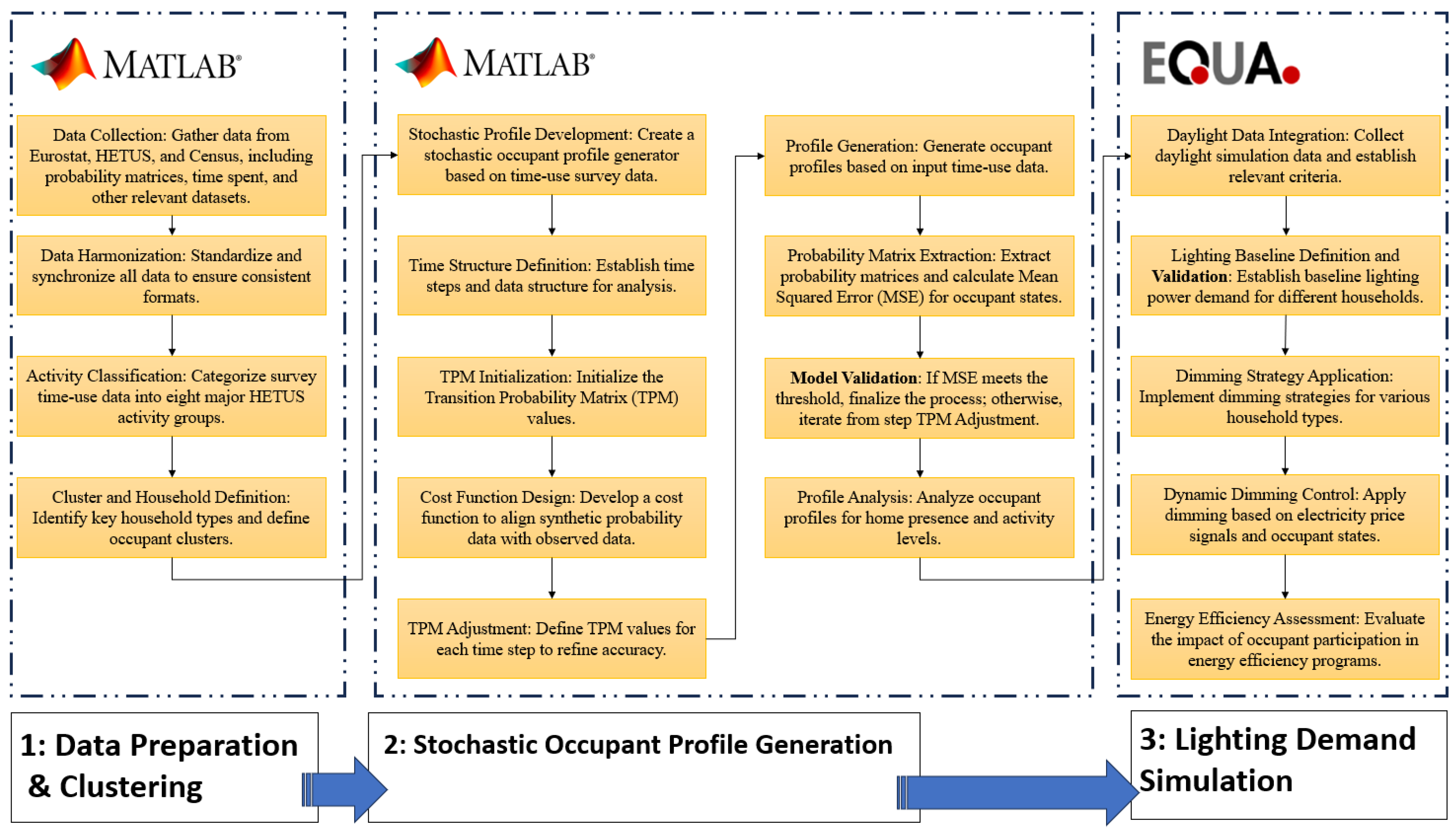
Figure 1. Framework for Stochastic Occupant Modeling and Energy Demand Simulation.
Energies 18 05133 g001
Figure 2. Comparison of activity probability patterns over time for empirical/reference TUS and simulated synthetic TUS data, showcasing the alignment of activity transitions throughout the day.
Energies 18 05133 g002
Figure 3. Comparison of time spent on daily activities: observed data vs. Markov chain models.
Energies 18 05133 g003
Figure 4. Dendrogram Representing Hierarchical Clustering of Groups.
Energies 18 05133 g004
Figure 5. Distribution of annual home occupancy hours across household groups.
Energies 18 05133 g005
Figure 6. Stochastic simulation of annual power demand for lighting by household type (kWh/year).
Energies 18 05133 g006
Figure 7. Impact of dimming strategies on annual household lighting demand (kWh).
Energies 18 05133 g007
Figure 8. Total lighting demand reduction under different dimming and participation levels (GWh).
Energies 18 05133 g008
Figure 9. Impact of price-based and activity-specific dimming on annual household lighting demand.
Energies 18 05133 g009
Figure 10. Impact of participation rate on total lighting demand under price-based and activity-based dimming.
Energies 18 05133 g010
Table 1. Comparison of Occupant Behavior Modelling Methods [11,32].
AspectDeterministic ModelsStochastic ModelsAgent-Based Modelling
ComplexityLowModerate to HighHigh
PredictabilityFixed outcomesGenerates a range of outcomesDynamic interactions
Data RequirementsLowHighModerate to High
RealismModerateHighVery High
Common Use CasesBasic and code complianceSensitivity analysis, DSMInteraction-heavy scenarios
Computational EffortLowHighVery High
Table 2. Summary of key studies on residential occupancy modelling and energy applications.
TitleYearCountryApplicationMethodUnique
Contribution
Typical occupancy profiles and behaviors in residential buildings in the United States [41]2020United StatesOccupancy schedulesProbabilisticU.S. homes energy modeling
Stochastic bottom-up load profile generator for Canadian households’ electricity demand [33]2023CanadaLoad profilesMarkov ChainsNon-HVAC load modeling
Room-level occupancy simulation model for private households [38]2020DenmarkRoom-level patternsHidden Markov ModelsFine-grained simulation
Four-state domestic building occupancy model for energy demand simulations [35]2018United KingdomOccupancy statesMarkov ChainsFour-state simulation
A Stochastic Model for Residential User Activity Simulation [39]2020DenmarkUser activityMarkov ChainsTUS data sequences
A method for the identification and modelling of realistic domestic occupancy sequences for building energy demand simulations and peer comparison [42]2019BelgiumRealistic patternsHierarchical ClusteringDaily consistency
A high-temporal resolution residential building occupancy model to generate high-temporal resolution heating load profiles of occupancy-integrated archetypes [43]2020United KingdomHeating load profilesMarkov ChainsStochastic diversity
Stochastic simulation of occupant-driven energy use in a bottom-up residential building stock model [37]2022United StatesEnergy usageMarkov Chains + SamplingATUS data integration
The Effect of Temporal Resolution on the Accuracy of Predicting Building Occupant behavior based on Markov Chain Models [44]2017United KingdomTemporal resolutionMarkov ChainsPrediction accuracy
Demand response included
From buildings to cities: How household demographics shape demand response and energy consumption [12]2024CanadaDemand responseMarkov ChainsImpact household types on demand response
Data-driven modelling of energy demand response behavior based on a large-scale residential trial [45]2021Australia
(SGSC data)
Demand responseMarkov ChainsPrediction of the households’ response behavior
Table 3. Demographic Categories: Household Composition, Employment, Education, and Age Groups [5].
Household & Family CompositionEmployment StatusEducationAge Groups
Couple 45 to 64 with no childrenPerson from 25 to 44 with no children (parents’ household)StudentsPrimary education (level 1)Age 15–20
Couple 45 with no childrenPerson—25 with no children (parents’ household)Full-time workersLower secondary education (level 2)Age 20–44
Couple +65 with no childrenPerson from 45 to 64 years old, not married and no childrenPart-time workersUpper secondary & post-secondary non-tertiary (3 & 4)Age 45–64
Couple with youngest child—6Person—45 in Not married and no childrenHomemakersFirst stage tertiary education (level 5A)Age 45–64
Couple with youngest child between 7 and 17Person +65, Not married and no childrenRetiredSecond stage tertiary education (level 6)Age 65+
Single parent with youngest child—18 UnemployedFirst stage tertiary education (level 5B)
Table 4. Mean Squared Error (MSE) values for activity categories, reflecting the accuracy of simulated synthetic data in replicating empirical patterns.
ActivityMSE
(Basic Markov Chain)
MSE
(Improved Markov Chain)
Personal Care0.910.038
Eating0.090.011
Work/Study0.500.011
Household Care0.320.098
Leisure0.240.050
TV0.520.035
Travel to Work/Study0.100.099
Unspecified0.080.011
Table 5. Demographic Groups and Their Assigned Clusters Based on Time-Use Patterns.
Group_1Cluster GroupCluster Group ClusterGroupCluster
65 years or over1From 20 to 24 years2Person under 25, no children under 18, living with parents2Level 2 education2
Homemakers1From 25 to 44 years2Person under 45 in a couple, no children under 182Levels 5A and 6 educations2
Other Jobs1From 45 to 64 years2Person under 45 in another household arrangement, no children under 182Level 5B education2
Retired persons1Person 25 to 44, no children under 18, living with parents2Single parent with youngest child under 182Levels 3 and 4 educations2
Unemployed persons1Person 45 to 64 in a couple, no children under 182Students2From 15 to 20 years2
Person 65 or over, in a couple, with no children younger than 181Person 45 to 64 in another household arrangement, no children under 182Working full-time2Person in a couple, youngest child under 62
Person 65 or over, living in another household arrangement, no children under 181Person in a couple, youngest child between 7 and 172Working part-time2Level 1 education2
Table 6. Descriptive statistics of annual home occupancy hours for different household groups.
GroupMean (Hour)StdDev (Hour)Min. (Hour)Max. (Hour)IQR (Hour)
Couple Retired77528474627999113
Couple with Child678510964237120145
Couple Working688411065647251144
Retired Persons77578474158004113
Working Full Time669210963347057148
Table 7. Statistical summary of annual power demand for lighting by household type.
GroupMean (kWh)StdDev (kWh)Min. (kWh)Max. (kWh)IQR (kWh)
Couple Retired2581122229514
Couple with Child180815320511
Couple Working147712316710
Retired Persons161813818610
Working Full Time12671071509
Disclaimer/Publisher’s Note: The statements, opinions and data contained in all publications are solely those of the individual author(s) and contributor(s) and not of MDPI and/or the editor(s). MDPI and/or the editor(s) disclaim responsibility for any injury to people or property resulting from any ideas, methods, instructions or products referred to in the content.