Enhanced Short-Term Photovoltaic Power Prediction Through Multi-Method Data Processing and SFOA-Optimized CNN-BiLSTM

Abstract

The increasing global demand for renewable energy poses significant challenges to grid stability due to the fluctuation and unpredictability of photovoltaic (PV) power generation. To enhance the accuracy of short-term PV power prediction, this study proposes an innovative integrated model that combines Convolutional Neural Networks (CNN) and Bidirectional Long Short-Term Memory (BiLSTM), optimized using the Starfish Optimization Algorithm (SFOA) and integrated with a multi-method data processing framework. To reduce input feature redundancy and improve prediction accuracy under different conditions, the K-means clustering algorithm is employed to classify past data into three typical weather scenarios. Empirical Mode Decomposition is utilized for multi-scale feature extraction, while Kernel Principal Component Analysis is applied to reduce data redundancy by extracting nonlinear principal components. A hybrid CNN-BiLSTM neural network is then constructed, with its hyperparameters optimized using SFOA to enhance feature extraction and sequence modeling capabilities. The experiments were carried out with historical data from a Chinese PV power station, and the results were compared with other existing prediction models. The results demonstrate that the Root Mean Square Error of PV power generation prediction for three scenarios are 9.8212, 12.4448, and 6.2017, respectively, outperforming all other comparative models.

1. Introduction

As the world places greater importance on environmental protection and sustainable development, the share of renewable energy in the energy mix has been growing steadily. Solar energy, acclaimed as a clean, emission-free, and sustainable resource, is an optimal choice for green energy development [1]. Photovoltaic (PV) power generation, the principal means of harnessing solar energy, is experiencing rapid growth. Nevertheless, PV output is affected by multiple factors, making it fluctuating and unpredictable. This variability challenges grid stability and dispatch [2]. Consequently, improving PV power forecasting and mitigating its grid impacts have become key to ensuring dependable and efficient system operation [3].

Traditional PV power prediction methods include physical models and statistical approaches, which have been widely studied [4]. Physical models rely on detailed meteorological and environmental factors, but they often suffer from high computational complexity and sensitivity to input accuracy [5]. Statistical methods like exponential smoothing [6], auto-regressive moving average [7], and autoregressive integrated moving average [8] capture historical patterns but struggle with nonlinear and complex relationships, degrading accuracy.

Deep learning techniques have garnered considerable attention for PV power prediction in recent years due to their powerful feature extraction and nonlinear modeling capabilities [9]. Many scholars have applied Convolutional Neural Networks (CNN) [10], gated recurrent units [11], and Long Short-Term Memory (LSTM) [12] to improve forecasting accuracy. Building on this, many studies adopt hybrid architectures. Zang et al. [13] proposed a spatiotemporal hybrid CNN-LSTM model for short-term solar radiation prediction and evaluated its performance in different seasons and weather conditions, showing its superior predictive ability. Limouni et al. [14] proposed an LSTM-TCN-based forecasting model to improve prediction accuracy, and the results demonstrated that the proposed model outperforms baseline and conventional models in forecasting accuracy. Li et al. [15] introduced a Stacking ensemble of optimized Neural Prophet, LSTM, and Informer models, which achieved good performance by delivering lower errors, improved stability across different forecasting horizons, and better adaptability to seasonal changes in solar power generation. However, deep learning models often face hyperparameter selection challenges, significantly affecting their performance.

To address this problem, scholars have explored various optimization algorithms to meet the challenge of optimizing deep learning parameters. Hou et al. [16] used the whale optimization algorithm (WOA) to optimize the training iterations, learning rate, and number of hidden neurons of the LSTM to enhance the prediction accuracy of the model. Li et al. [17] proposed a short-term PV power generation prediction method by combining the sparrow search algorithm (SSA) and BiLSTM, and verified its effectiveness by comparing it under different seasons and weather. Zhou et al. [18] utilized the RIME optimization algorithm (RIME) to modify the hyperparameters of neural networks and proved the capability of RIME in short-term photovoltaic power prediction. Zhang et al. [19] introduced a short-term PV forecasting model based on a secondary decomposition method, and optimized the BiLSTM hyperparameters using the Crested Porcupine Optimization algorithm (CPO). The results showed that CPO effectively tuned the model parameters, leading to improved forecasting performance. However, these algorithms still have some drawbacks, such as long optimization times and the risk of falling into local optima, resulting in suboptimal performance.

Further, data quality is another key factor that directly affects the accuracy of power prediction. The power generation data series is a non-smooth, non-linear signal with various time scales and contains numerous hidden patterns. Integrating signal decomposition and dimensionality reduction methods with deep learning can improve the accuracy of power predictions. Wang et al. [20] proposed a PCA-SSA-VMD-based hybrid model to enhance offshore wind power forecasting for economic scheduling and demonstrated that the proposed model effectively enhances prediction precision and validates its effectiveness. Zhang et al. [21] proposed a combined model that combines Empirical Mode Decomposition (EMD) and Kernel Principal Component Analysis (KPCA) for data preprocessing with a deep learning framework for wind power forecasting, achieving superior prediction accuracy compared to benchmark models. Peng et al. [22] developed a hybrid model that combines symplectic geometry model decomposition, KPCA, and an optimized BiLSTM, achieving highly accurate forecasts of wind and photovoltaic power. However, this method is rarely used for PV power forecasting.

Based on the analysis above, this research proposes a hybrid prediction framework that combines data classification, selection, and optimization algorithms with neural networks. The main contributions and innovations are summarized as follows:

(1)

Classify the data into multiple categories by using clustering and construct differentiated prediction models for various weather conditions to improve the model’s adaptability to complex weather.

(2)

The feature data are decomposed by using EMD and downscaled by using KPCA to extract key features, reduce redundancy, and improve computational efficiency. The processed model is then compared with the unprocessed counterpart to verify its advantages in improving the stability of PV power forecasting and its adaptability to complex meteorological conditions.

(3)

The SFOA is first introduced into the field of photovoltaic forecasting to automatically optimize the hyperparameters of models. It is compared with other optimization algorithms, demonstrating its advantage in improving the generalization ability of photovoltaic forecasting models.

The rest of the paper is arranged as follows: Section 2 describes the principle behind each method employed. Section 3 introduces the prediction model and details the experimental steps. Section 4 shows the experimental data along with the analysis methodology. Section 5 shows the numerical results and compares them with alternative methods. Section 6 provides the conclusions and points out issues for further research.

2. Principle

2.1. K-Means Clustering Algorithm

K-means is a widely used clustering algorithm that divides a dataset into $K$ clusters by minimizing within-cluster variance. The specific procedure is as follows:

Step 1: Given data $D=\{x_1,x_2,\dots ,x_N\}$, randomly initialize $K$ centroids $\{c_1,c_2,\dots ,c_K\}$.

Step 2: For each data point $x_i\in D$, compute its Euclidean distance from each cluster centroids ${c }_j$ by using the formula $d(x_i,{c }_j)=\parallel x_i-{c }_j \parallel$. Each data point is then allocated to the cluster corresponding to the nearest centroid. This results in $K$ clusters, where each data point $x_i$ is assigned to the cluster whose centroid is closest.

Step 3: After assigning all data points to their respective clusters, the centroids of the clusters are recalculated. The new centroid ${c }_j$ for each cluster ${C }_j$ is computed as the mean of the data points in that cluster:

$${c }_j={\displaystyle \frac{1}{\left|C_j\right|}}\sum _{x_i\in C_j}{x}_i$$

(1)

where ${c }_j$ is the set of data points in cluster $j$, and $\left|{C }_j\right|$ is the number of points in the cluster.

Step 4: Steps 2 and 3 are repeated until the cluster centroids stabilize, or the maximum number of iterations is reached, indicating the algorithm’s convergence.

2.2. Empirical Mode Decomposition

EMD is a decomposition method for nonlinear, non-smooth signals, breaking the signal into intrinsic modal functions (IMFs) that capture oscillatory components at different time scales. The specific decomposition process is as follows:

Step 1: Given a signal $x(t)$, the first step is to identify the local extrema. These extrema points are used to construct the lower and upper envelopes of the signal, denoted as $u(t)$ and $l(t)$, respectively.

Step 2: The local mean $m(t)$ is calculated as the average of these envelopes. The first component is $h_1(t)=x(t)-m(t)$. If $h_1(t)$ satisfies the stopping criteria, which requires equal numbers of extrema and zero-crossings, it is considered the first IMF.

Step 3: The residual $r_1(t)=x(t)-h_1(t)$ becomes the new signal, and the procedure repeats to find further IMFs, continuing until the residual $r_n(t)$ meets the termination condition.

Step 4: The decomposition stops when the residual signal $r_n(t)$ becomes monotonic or reaches a predefined threshold $\delta (t)$. The final decomposition is:

$$x(t)=h_1(t)+h_2(t)+\cdots +h_n(t)+r_n(t)$$

(2)

where $h_1(t)$, $h_2(t)$,…, $h_n(t)$ are the IMFs, and $r_n(t)$ is the residual.

2.3. Kernel Principal Component Analysis

After signal decomposition, the increased input dimension can complicate the model and reduce its generalization ability. KPCA employs a kernel function to transform data into a high dimensional feature space for nonlinear dimensionality reduction. In this space, principal component analysis is applied to extract the key features of the data. Unlike traditional PCA, KPCA enables nonlinear feature extraction by leveraging the kernel function, which avoids high-dimensional mapping. The specific procedure is as follows:

Step 1: Select a kernel function and map the original data into a high-dimensional space, obtaining the corresponding data matrix. The polynomial kernel function is defined as:

$$K(x_i,x_j)=\phi {(x_i)}^d\phi (x_j)$$

(3)

where $x_i$, $x_j$ are original data samples, and $d$ is the degree of the highest-order term.

Step 2: Center the kernel matrix and obtain the centered kernel matrix $K_c$. The equation is presented below:

$$K_c=K-I_{N}K-K{I}_N+I_{N}K{I}_N$$

(4)

where $I_N$ represents an $N\times N$ matrix whose elements are all $1/N$.

Step 3: Calculate the eigenvalues and eigenvectors of the centered kernel matrix.

Step 4: The cumulative contribution of the eigenvalues $r_1,r_2,\dots ,r_n$ is calculated to quantify the contribution of each eigenvalue to the total variability of the data. When the cumulative contribution $r_t$ reaches a predefined threshold $p$, the top $t$ principal components $a_1,a_2,\dots ,a_t$ are selected as the reduced-dimensional representation of the data.

2.4. SFOA-CNN-BiLSTM Model

2.4.1. CNN-BiLSTM Neural Network Model

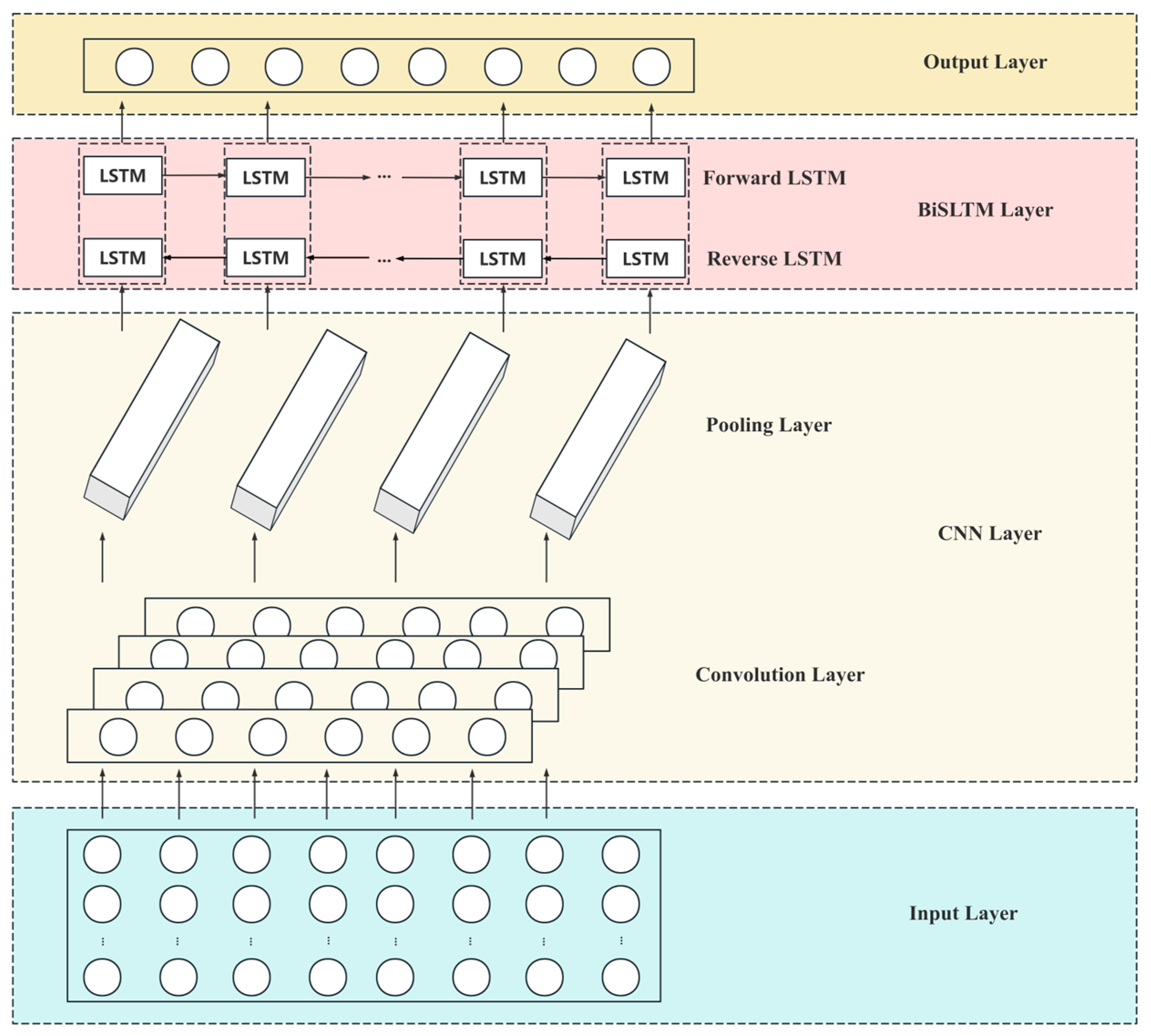
The CNN-BiLSTM model is a hybrid architecture combining Convolutional Neural Networks and Bidirectional Long Short-Term Memory Networks. This architecture leverages the strengths of both models, making it particularly effective for tasks like sequential data analysis.

(1)

CNN Layer

In the CNN layer, multiple convolutional layers are used to automatically capture spatial hierarchies and local patterns from the input data. These layers apply convolutional filters, generating feature maps that capture local dependencies and patterns. The CNN layer for a single filter $w$ applied to an input sequence $x$ can be expressed as:

$$y=f(x\ast w+b)$$

(5)

where $x$ represents the input sequence, $w$ represents the convolutional filter, $b$ represents the bias term, and $f$ represents an activation function.

(2)

BiLSTM Layer

The BiLSTM layer is employed to capture the sequential dependencies in the data. Unlike traditional LSTMs that capture only past information, BiLSTM networks capture sequence information by processing data bidirectionally. This enables them to capture information from both the past and the future, making them particularly effective for tasks that require understanding both preceding and succeeding elements. A single LSTM unit computes the following relations:

$$i_t=\sigma (W_i\cdot [h_{t-1},x_t]+b_i)$$

(6)

$$f_t=\sigma (W_f\cdot [h_{t-1},x_t]+b_f)$$

(7)

$$o_t=\sigma (W_o\cdot [h_{t-1},x_t]+b_o)$$

(8)

$$c_t=f_t\ast c_{t-1}+i_t\ast \tanh (W_c\cdot [h_{t-1},x_t]+b_c)$$

(9)

$$h_t=o_t\ast \tanh (c_t)$$

(10)

where $i_t$, $f_t$, $o_t$ are the input, forget, and output gates, respectively, $h_t$ is the hidden state, $c_t$ is the cell state, $W$ are the weights and $b$ are the biases, $x_t$ is the current input, and $h_{t-1}$ is the previous hidden state.

The BiLSTM can process the input sequence in two directions. The outputs of both directions are then concatenated to provide a more comprehensive representation of the sequence. For each time step $t$, the hidden state $h_t$ of the BiLSTM output is a splice of the forward and reverse LSTM outputs:

$$h_t=[\overrightarrow{h_t},\overleftarrow{h_t}]$$

(11)

where $\overrightarrow{h_t}$ and $\overleftarrow{h_t}$ indicate the forward and reverse LSTM outputs at time step $t$, respectively.

(3)

Overall CNN-BiLSTM Structure

In the CNN-BiLSTM model, the CNN layers initially extract local features from the input sequence. These features are then passed to the BiLSTM layers, which model the temporal dependencies of the sequence in both directions. The specific model parameters are presented in

Table 1. Parameter configuration of the overall model.

Parameter	Value
Input layer time steps	8
Output layer variables	1
Maximum number of iterations	200
Maximum number of epochs	200
CNN layers	2
BiLSTM layers	3
Optimizer	Adam
Activation function	ReLU
Initial learning rate	0.01
L2 Regularization	0.002

, and the structure of the CNN-BiLSTM model is depicted in Figure 1.

2.4.2. SFOA Principle

SFOA is a novel bio-inspired metaheuristic inspired by the behaviors of starfish, including exploration, preying, and regeneration [23]. It employs a hybrid search strategy that integrates both five-dimensional and unidimensional search patterns. This integration can not only optimize resource utilization but also significantly enhance computational efficiency, enabling SFOA to swiftly and accurately navigate through complex solution spaces and identify optimal solutions more effortlessly. The main ideas of SFOA are expressed as follows:

(1)

Initialization

$$X_{ij}=l_j+r(u_j-l_j),i=1,2,\dots ,N,j=1,2,\dots ,D$$

(12)

where $X_{ij}$ denotes the $j^{\mathrm{th}}$ dimensional position of the $i^{\mathrm{th}}$ starfish, $r$ denotes a random number between (0, 1), $u_j$ and $l_j$ are bounds of the $j^{\mathrm{th}}$ dimensional design variable, respectively.

(2)

Exploration phase

If the optimization problem has a dimension greater than 5, SFOA uses the following mathematical model:

$$Y_{i,p}^T=X_{i,p}^T+a_1(X_{i,p}^T-X_{i,p}^T)\cos \theta ,r\le 0.5$$

(13)

$$Y_{i,p}^T=X_{i,p}^T-a_1(X_{\mathrm{best},p}^T-X_{i,p}^T)\sin \theta ,r>0.5$$

(14)

$$a_1=(2r-1)\pi$$

(15)

$$\theta ={\displaystyle \frac{\pi }{2}}\cdot {\displaystyle \frac{T}{T_{\max }}}$$

(16)

where $Y_{i,p}^T$ and $X_{i,p}^T$ denote the obtained position and the current position of a starfish, respectively; $X_{\mathrm{best},p}^T$ denotes the $p$-dimension of the best current position, $p$ is a randomly selected 5-dimension in the $D$-dimension, $r$ denotes the random number between (0, 1); $T$ is the current number of iterations, and $T_{\max }$ is the maximal number of iterations, $\theta$ is in the range of [0, $\pi /2$].

If the optimization problem has no dimension greater than 5, the exploration phase uses a one-dimensional search pattern to update the position.

$$Y_{i,q}^T=E_t{X}_{i,p}^T+A_1(X_{k_1,p}^T-X_{i,p}^T)+A_2(X_{k_2,p}^T-X_{i,p}^T)$$

(17)

$$E_t={\displaystyle \frac{T_{\max }-T}{T_{\max }}}\cos \theta$$

(18)

where $X_{k_1,p}^T$ and $X_{k_2,p}^T$ are the positions of two randomly chosen starfish in the p-dimension, $A_1$ and $A_2$ are two random numbers between (−1, 1), and $p$ is a randomly chosen number in the $D$ dimension.

(3)

Exploitation phase

SFOA employs a parallel bidirectional search strategy, which leverages information from other starfish and the current best position within the population. The distances can be calculated as:

$$d_m=(X_{\mathrm{best}}^T-X_{m_p}^T),m=1,\dots ,5$$

(19)

where $d_m$ represents the five distances between the global best and other starfish, and ${\mathrm{m}}_{\mathrm{p}}$ refers to five randomly selected starfish. The first update rule for each starfish is modeled as follows:

$$Y_i^T=X_i^T+r_1{d}_{m1}+r_2{d}_{m2}$$

(20)

where $r_1$ and $r_2$ are random numbers between (0, 1), $d_{m1}$ and $d_{m2}$ are randomly selected in $d_m$. In addition, if $i=N$, another update rule is modeled as follows:

$$Y_i^T=\exp \left(-{\displaystyle \frac{T\times N}{T_{\max }}}\right)X_i^T$$

(21)

where $T$ is the current iteration, $T_{\max }$ is the maximum iterative number, and $N$ is the population size.

2.4.3. The Steps of the SFOA-CNN-BiLSTM Model

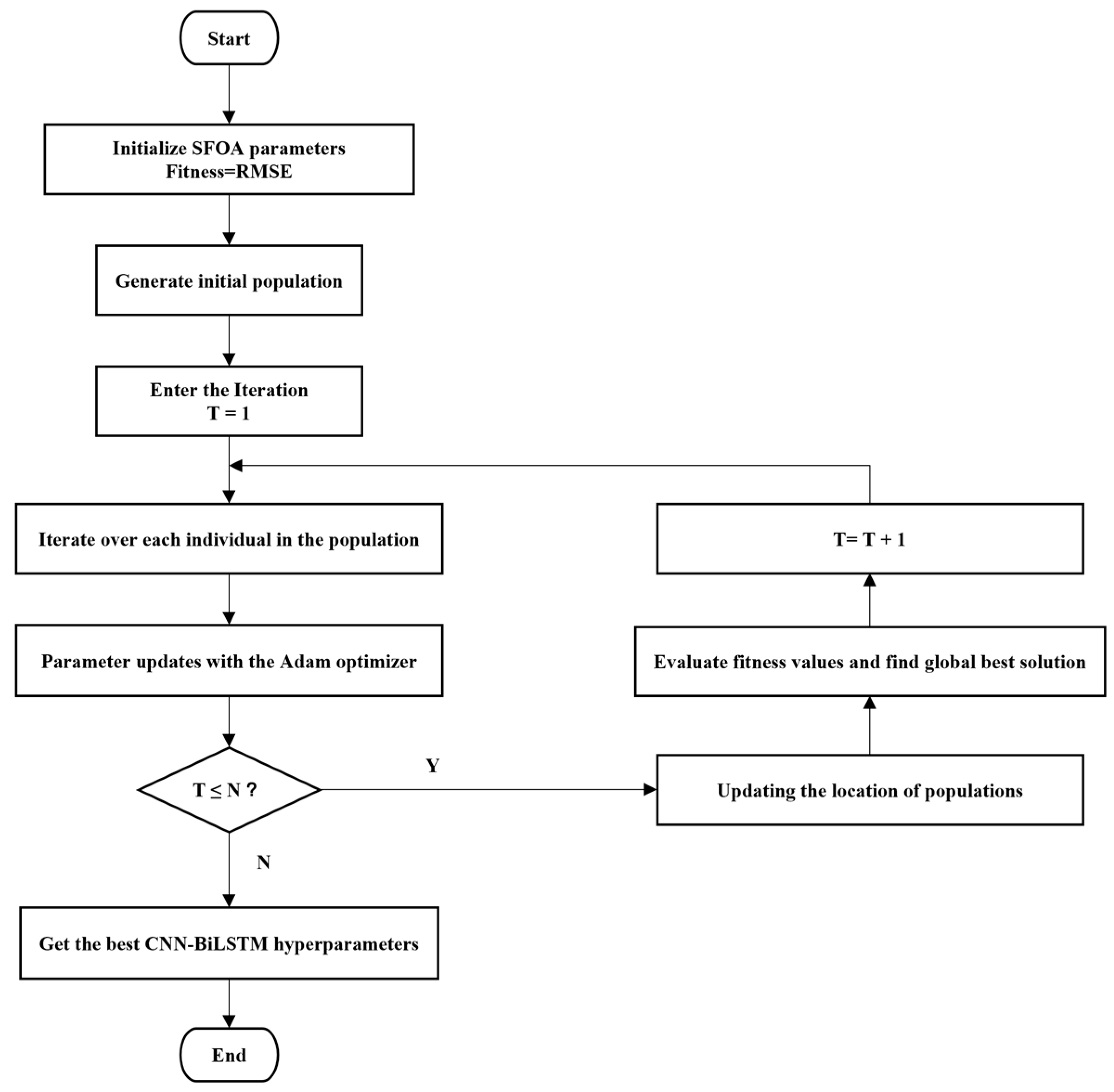
The network performance and convergence speed are determined by the values of its hyperparameters, which can be optimized by SFOA. The main steps in the SFOA optimization of networks are as follows:

Step 1: Determine the optimized hyperparameter range and initialize the SFOA population.

Step 2: Select RMSE as the fitness function.

Step 3: Entering the optimization phase of the SFOA, the process undergoes iterative optimization through two distinct stages.

Step 4: Check the stopping condition. If the maximum number of iterations is reached, the optimization process stops.

Step 5: Obtain the best set of hyperparameters.

Figure 2 shows the steps of optimization of CNN-BiLSTM using SFOA.

2.5. Evaluation Metrics

To assess the model’s performance, six performance metrics are used in this study: RMSE, Mean Squared Error (MSE), Mean Absolute Error (MAE), Mean Absolute Percentage Error (MAPE), Pearson Correlation Coefficient (R), and Coefficient of Determination (R²). These metrics are commonly used to assess the accuracy and reliability of forecasting models. The detailed equations for each metric are expressed as follows:

$$\mathrm{RMSE}=\sqrt{{\displaystyle \frac{1}{n}}\sum _{i=1}^n{(y_i-{\widehat{y}}_i)}^2}$$

(22)

$$\mathrm{MSE}={\displaystyle \frac{1}{n}}\sum _{i=1}^n{(y_i-{\widehat{y}}_i)}^2$$

(23)

$$\mathrm{MAE}={\displaystyle \frac{1}{n}}\sum _{i=1}^n|y_i-{\widehat{y}}_i|$$

(24)

$$\mathrm{MAPE}={\displaystyle \frac{1}{n}}\sum _{i=1}^n\left|{\displaystyle \frac{y_i-{\widehat{y}}_i}{y_i}}\right|\times 100\%$$

(25)

$$\mathrm{R}={\displaystyle \frac{{\displaystyle \sum _{i=1}^n}(y_i-\overline{y})({\widehat{y}}_i-\overline{\widehat{y}})}{\sqrt{{\displaystyle \sum _{i=1}^n}{(y_i-\overline{y})}^2{\displaystyle \sum _{i=1}^n}{({\widehat{y}}_i-\overline{\widehat{y}})}^2}}}$$

(26)

$${\mathrm{R}}^2=1-{\displaystyle \frac{{\displaystyle \sum _{i=1}^n}{(y_i-{\widehat{y}}_i)}^2}{{\displaystyle \sum _{i=1}^n}{(y_i-\overline{y})}^2}}$$

(27)

where $n$ is the number of samples, $y_i$ is the real power value, ${\widehat{y}}_i$ is the predicted power value, and $\overline{y}$ is the average power value.

3. PV Power Prediction Based on the Developed Fusion Method

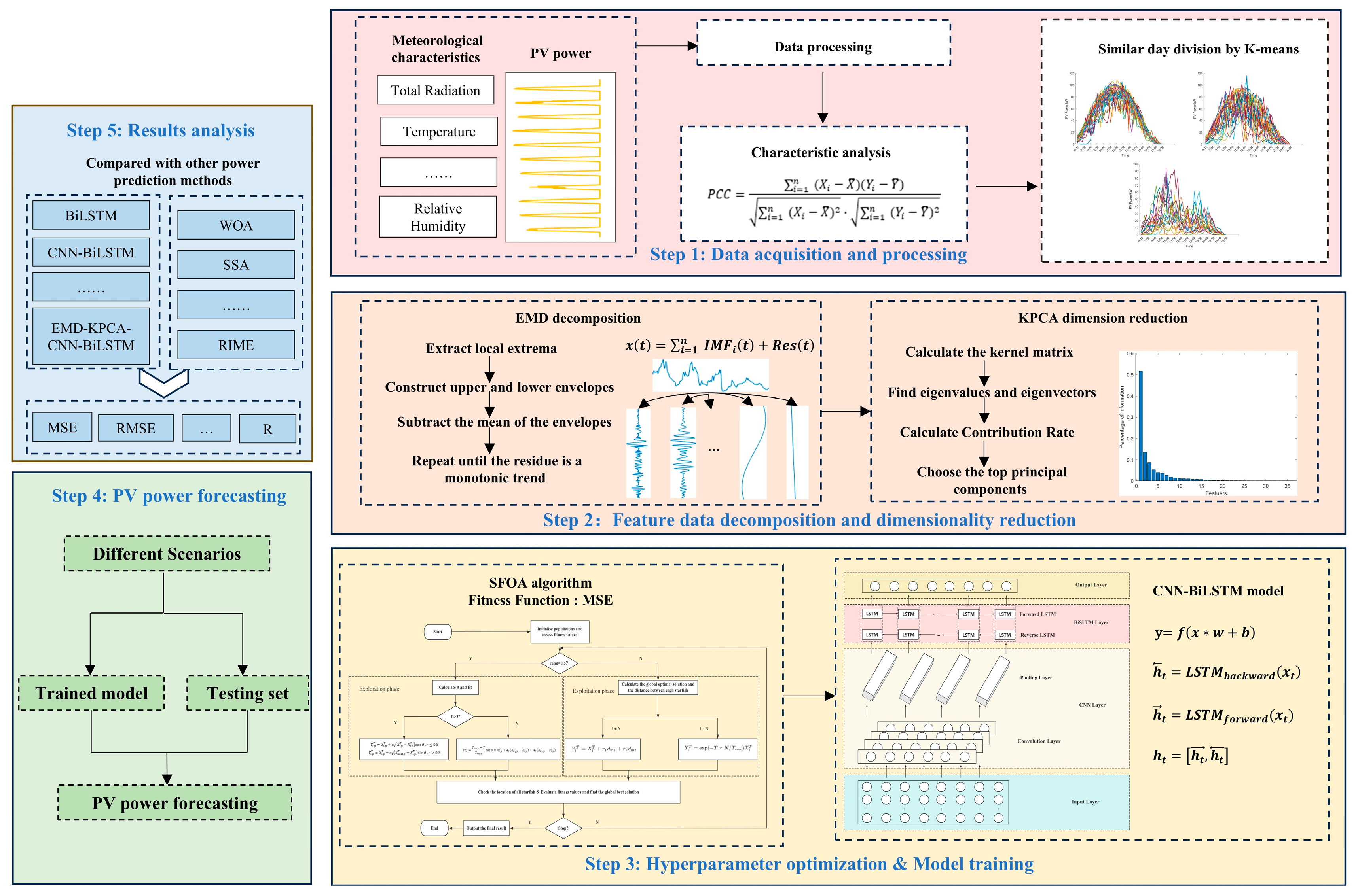
In this paper, a fusion method for PV power prediction based on similar day clustering with EMD-KPCA-SFOA-CNN-BiLSTM is developed. The main steps are illustrated in Figure 3 and they are described as follows:

Step 1: Data acquisition and processing. The raw power generation dataset is first preprocessed and the most representative feature parameters are screened by correlation coefficient analysis. Then, a similar day clustering method is used to group the data.

Step 2: Feature data decomposition and dimensionality reduction. The feature data is first decomposed by using EMD. Subsequently, KPCA is applied to reduce dimensionality to obtain the principal components affecting the PV output power.

Step 3: Hyperparameter optimization and model training. In training the CNN-BiLSTM model, the SFOA is employed to optimize key hyperparameters to enhance overall model performance.

Step 4: PV power forecasting. During the forecasting stage, the preprocessed data is input into the neural network with optimized hyperparameters to generate short-term PV power predictions.

Step 5: Results analysis. Different evaluation metrics are used to judge the prediction results and to validate the advantages of the developed fusion method in comparison with other prediction methods.

4. Data Analysis and Prediction Process

4.1. Data Description and Preprocessing

The experiments were conducted on a system running Windows 11, equipped with an AMD Ryzen 7 5800H processor and an NVIDIA GeForce RTX 3050 GPU. All experiments were executed using MATLAB 2021b, with GPU acceleration enabled for enhanced computational performance.

The photovoltaic power generation data used in the study were collected from a power station in China, with a total of 92 days of records gathered from June to August 2017. The data was collected every 15 min. However, since the system does not generate power at night, only the period from 6:00 AM to 7:00 PM is included and this gives 52 data points per day. The collected data were as follows: total radiation, direct radiation, scattered radiation, component temperature, temperature, pressure, relative humidity, and PV power generation.

During the process of collecting or transmitting the raw photovoltaic power generation data, data loss and abnormal fluctuations may occur. In this study, missing values and outliers are filled or replaced with the average values from the corresponding time points before and after the problematic data points. The descriptions of the data items in the database are presented in

Table 2. Variable definitions in the Database.

Variables	Unit	Min. Value	Max. Value
Total Radiation	W/m2	0	927.67
Direct Radiation	W/m2	0	853.4564
Scattered Radiation	W/m2	0	89.0563
Component Temperature	°C	16	53.8
Temperature	°C	0	40.7
Pressure	hPa	997.8	1020
Relative Humidity	%	0	116.5395

.

4.2. Characteristic Analysis

To analyze the relationship between the extracted features and their predictive ability, we used the Pearson correlation coefficient (PCC) to examine the correlation between each feature and the PV power. By calculating the PCC for each feature with the PV power, we can identify which features have higher predictive value in short-term PV power forecasting models. The calculation method for the PCC is shown as follow.

$$\mathrm{PCC}={\displaystyle \frac{{\displaystyle \sum _{i=1}^n}(X_i-\overline{X})(Y_i-\overline{Y})}{\sqrt{{\displaystyle \sum _{i=1}^n}{(X_i-\overline{X})}^2}\cdot \sqrt{{\displaystyle \sum _{i=1}^n}{(Y_i-\overline{Y})}^2}}}$$

(28)

where $X_i$ is the different values of feature $X$, $Y_i$ is the different values of feature $Y$, $\overline{X}$ is the mean value of feature $X$, and $\overline{Y}$ is the mean value of feature $Y$.

The result of the PCC between the environmental factors and PV power is displayed in

Table 3. The results of PCC.

Features	PCC
Total Radiation	0.538
Direct Radiation	0.538
Scattered Radiation	0.538
Component Temperature	0.292
Temperature	0.074
Pressure	0.055
Relative Humidity	−0.011

. A PCC value closer to 1 indicates a stronger correlation between the features and the PV power.

As can be seen from Table 3, the correlation between total radiation, direct radiation, scattered radiation, and component temperature with PV power is strong. Therefore, these features were selected as the input features for the subsequent sessions (Feature I: Total Radiation, Feature II: Direct Radiation, Feature III: Scattered Radiation, Feature IV: Component Temperature).

4.3. Similar Day Division

In practice, weather conditions impact PV power generation in various ways. To account for this, we applied the k-means clustering algorithm to group the data based on different weather scenarios. This classification allows the subsequent models to make more accurate predictions tailored to specific weather conditions. Through clustering, the 92 days of data are divided into three typical PV output day scenarios: Scenario I includes 41 typical days, representing strong sunlight and sunny weather. Scenario II includes 32 typical days, representing moderate sunlight and cloudy weather. Scenario III includes 19 typical days, representing weak sunlight and rainy weather. Figure 4 shows the results of the k-means clustering algorithm.

4.4. Analysis of the EMD Results

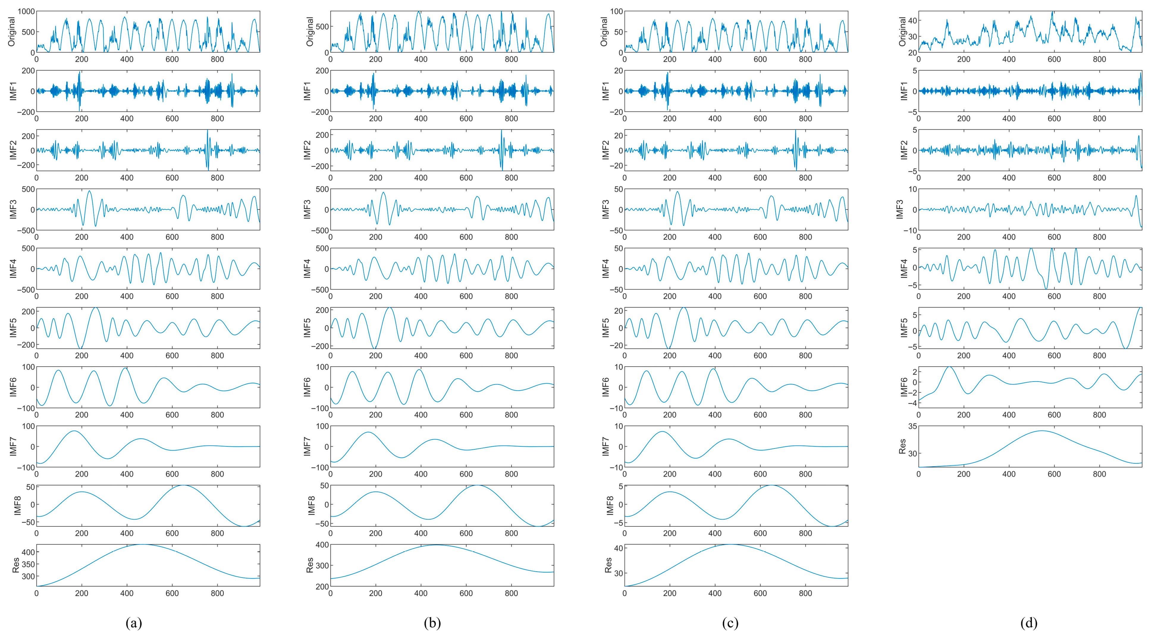
In this section, building upon the previous analyses, we further applied EMD to decompose the four features and obtain the IMF components and residual components for each feature under different scenarios. Taking Scenario III as an example, Figure 5 illustrates the decomposition results of EMD. For all three scenarios, the results of the EMD for the four features are presented in

Table 4. The results of the EMD.

Scenarios	Features	IMFs	Residual Components
Scenario I	Feature I	9	1
	Feature II	9	1
	Feature III	9	1
	Feature IV	9	1
Scenario II	Feature I	8	1
	Feature II	8	1
	Feature III	8	1
	Feature IV	8	1
Scenario III	Feature I	8	1
	Feature II	8	1
	Feature III	8	1
	Feature IV	6	1

.

4.5. KPCA Dimension Reduction

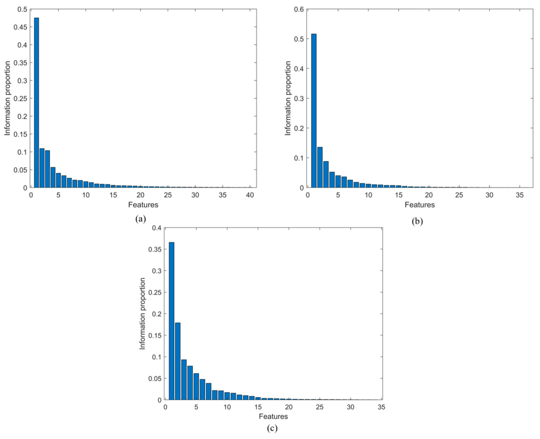
The IMF components obtained from EMD may exhibit high-dimensional redundancy and nonlinear coupling, which can lead to dimensionality issues and increase the risk of overfitting when directly used in prediction models. To better capture the nonlinear relationships between the features and reduce model complexity, we applied kernel principal component analysis to the feature sequence data. We selected components with a cumulative contribution greater than 90%, ensuring that the selected principal components more effectively portray the original data and enhance information synthesis. The processed data were subsequently employed as input samples for predicting future PV output power. Figure 6 illustrates the proportion of information captured by using KPCA across the three scenarios and

Table 5. The results of the KPCA dimensionality reduction.

Scenarios	Number of Components After KPCA
Scenario I	10
Scenario II	8
Scenario III	9

shows the number of components of each scenario after the KPCA dimensionality reduction.

4.6. Model Hyperparameter Settings

In this section, based on the CNN-BiLSTM neural network, the optimal hyperparameters of the network model are obtained by using SFOA computation to enhance the model performance and prediction accuracy. The hyperparameters optimized by the SFOA include the learning rate, dropout rate, the filters’ number in each CNN layer, the hidden units’ number in each BiLSTM layer, and the regularization parameters. In addition, we chose MSE loss as the loss function and the parameters are solved and continuously updated by using the Adam solver. The optimization range of hyperparameters is shown in

Table 6. Hyperparameters and the corresponding tuning ranges.

Hyperparameter	Range
Learning rate	[0.001, 0.01]
CNN 1 number of filters	[5, 20]
CNN 2 number of filters	[5, 20]
BiLSTM 1 number of hidden units	[5, 100]
BiLSTM 2 number of hidden units	[5, 100]
BiLSTM 3 number of hidden units	[5, 100]
Regularization parameter	[0.001, 0.01]
Dropout rate	[0.1, 0.5]

Note: Superscripts ^1–3 denote the layer index in the network (e.g., BiLSTM ¹, BiLSTM ², BiLSTM ³ correspond to the 1st, 2nd, and 3rd BiLSTM layers).

.

The dimensionality-reduced feature data and historical photovoltaic power were input into the CNN-BiLSTM model optimized by SFOA. We divided the dataset into training and testing sets at a ratio of 8:2.

5. Results and Discussions

5.1. Compared with Other Power Prediction Models

To validate the predictive effectiveness and high accuracy of the combined model, we employed five different models to make predictions on the test sets of three distinct scenarios. The prediction models used in this section are listed below: ① Model I: BiLSTM; ② Model II: CNN-BiLSTM; ③ Model III: EMD-KPCA-CNN-BiLSTM; ④ Model IV:SFOA-CNN-BiLSTM; and ⑤ Model V:EMD-KPCA-SFOA-CNN-BiLSTM. In the three scenarios, we chose August 18, August 19, and August 27, and Figure 7 shows the single-day prediction results of each model in the three different scenarios. At the same time,

Table 7. Prediction evaluation of five models in three scenarios.

Scenarios	Models	RMSE	MSE	MAE	MAPE	R	R2
Scenario I	Model I	13.0366	169.9517	10.5994	1.0915	0.9310	0.8401
	Model II	10.9585	120.0886	8.1677	0.7738	0.9476	0.8870
	Model III	10.4462	109.1226	7.4989	0.6053	0.9509	0.8973
	Model IV	10.0626	101.2558	7.2779	0.4846	0.9521	0.9047
	Model V	9.8212	96.4561	6.7460	0.3821	0.9546	0.9092
Scenario II	Model I	16.1908	262.1436	12.6917	2.7439	0.8649	0.7076
	Model II	14.1580	200.4482	10.7998	2.7218	0.8996	0.7764
	Model III	13.7453	188.9336	10.0814	2.0379	0.9049	0.7893
	Model IV	12.8802	165.8990	9.0924	2.1277	0.9122	0.8150
	Model V	12.4448	154.8726	8.7285	1.3895	0.9167	0.8273
Scenario III	Model II	6.9373	48.1260	5.4790	1.9408	0.8015	0.5982
	Model III	6.7524	45.5948	5.4117	1.5985	0.8107	0.6193
	Model IV	6.3657	40.5218	4.8873	1.3051	0.8222	0.6617
	Model V	6.2017	38.4616	4.4883	1.0829	0.8317	0.6789

shows the evaluation metrics for the prediction results across the entire test set (the results for Scenario III with Model I are excluded because of its poor performance).

By analyzing the results from the table, it can be obtained that:

(1)

The CNN-BiLSTM model improves its performance by adding a Convolutional Neural Network on the top of BiLSTM, and it helps the model extract more advanced information from local features. Compared with the single BiLSTM model, there is a significant improvement in all indicators, which proves the effectiveness of the CNN layer in enhancing the feature extraction ability of the model.

(2)

The EMD-KPCA-CNN-BiLSTM model adds EMD and KPCA techniques to the CNN-BiLSTM model. The RMSEs in the three scenarios decreased by 4.67%, 2.91%, and 2.67%, while the MAEs decreased by 8.19%, 6.65%, and 1.23%, respectively. This demonstrates that the combination of EMD and KPCA effectively reduces dimensionality while preserving the key information in the data, thereby lowering computational complexity and enhancing prediction performance.

(3)

The SFOA-CNN-BiLSTM model optimizes hyperparameters to further enhance performance. SFOA significantly reduces errors, leading to substantial improvements in RMSE, MSE, MAE, and MAPE.

(4)

The EMD-KPCA-SFOA-CNN-BiLSTM model combines four methods to maximize the performance. The model can handle complex time series data efficiently and performs the best among all the models. All the metrics are optimal in different scenarios, which proves its superiority.

5.2. Compared with Other Optimization Algorithms

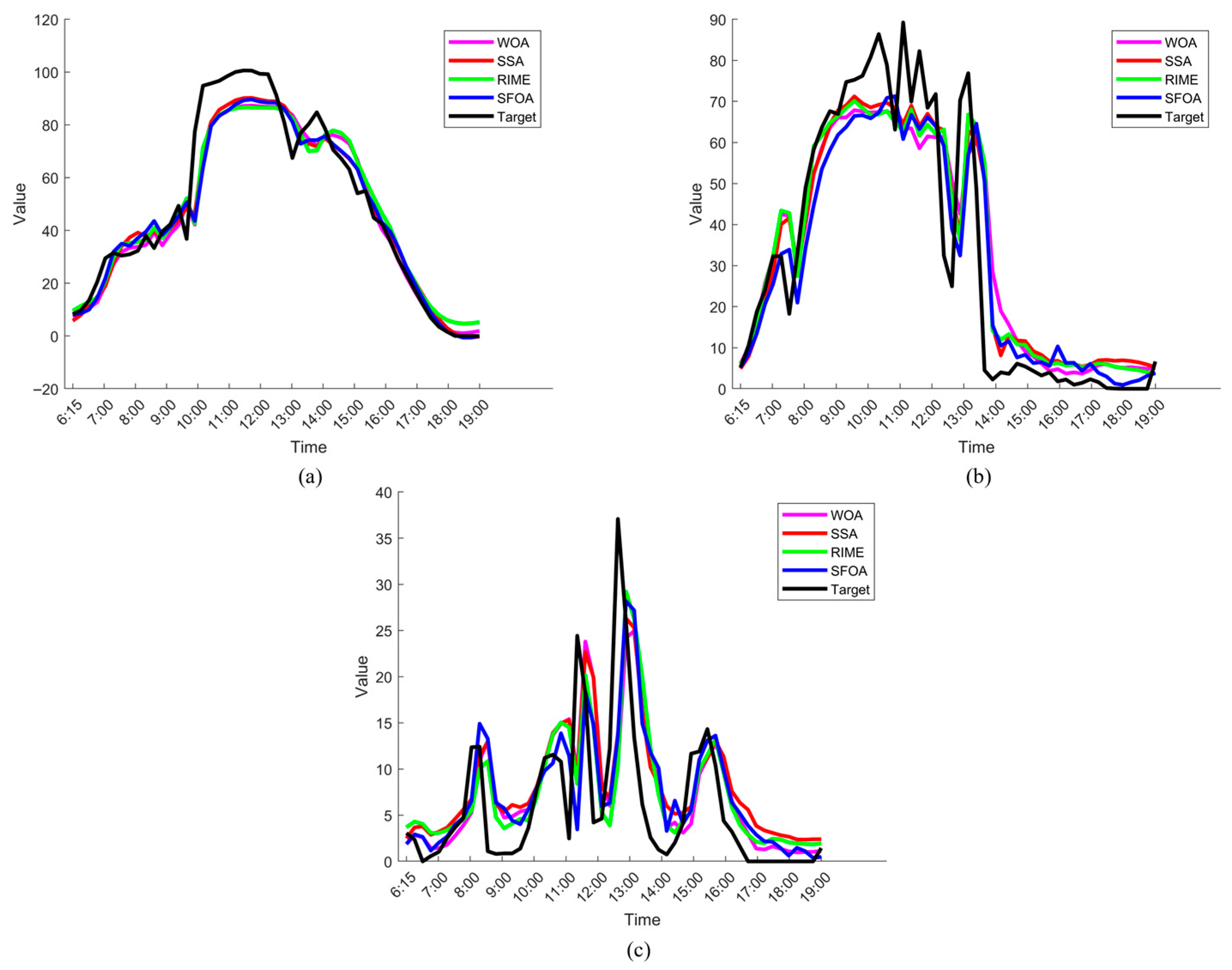
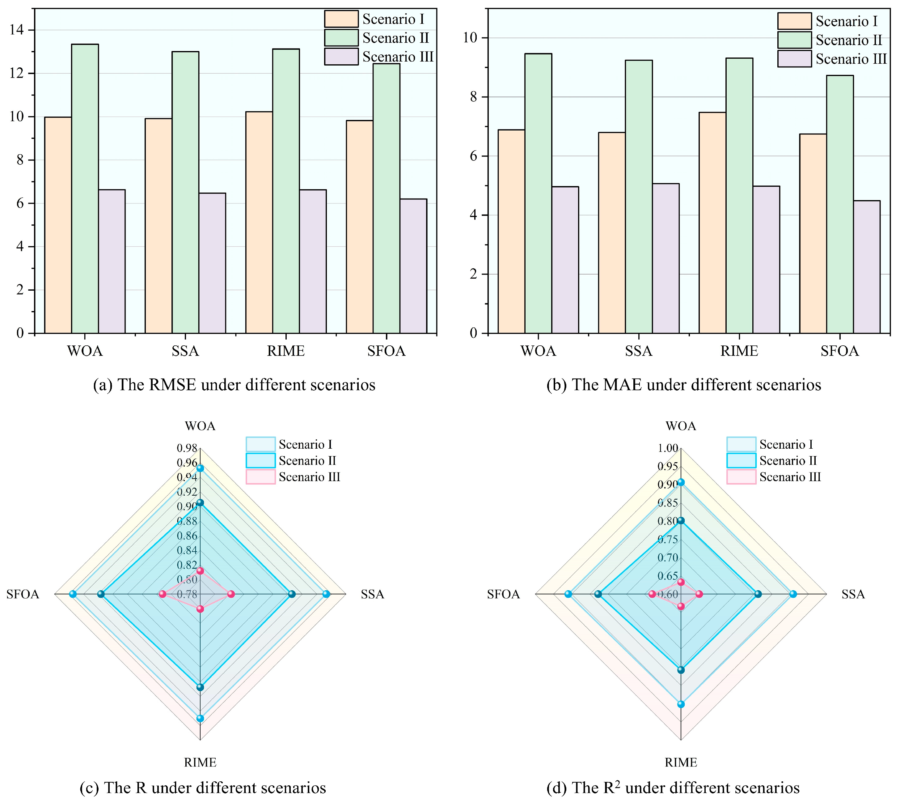
To verify the superiority of SFOA in dealing with short-term PV power forecasting problems, we used three other typical optimization algorithm methods to replace SFOA in Model V above, all of which have demonstrated effective optimization results in PV forecasting. The comparison optimization methods used in the section are listed below: ① WOA; ② SSA; and ③ RIME. Figure 8 shows the same single-day prediction results as in the previous section for each method for three different scenarios and

Table 8. Comparison results with other algorithm methods.

Scenarios	Methods	RMSE	MSE	MAE	MAPE	R	R2
Scenario I	WOA	9.9830	99.6602	6.8876	0.3444	0.9522	0.9062
	SSA	9.9087	98.1822	6.7963	0.4386	0.9527	0.9076
	RIME	10.2335	104.7254	7.4805	0.6014	0.9501	0.9014
	SFOA	9.8212	96.4561	6.7460	0.3821	0.9546	0.9092
Scenario II	WOA	13.3452	178.095	9.4649	1.8445	0.9051	0.8014
	SSA	13.0029	169.0742	9.2486	1.9398	0.9057	0.8114
	RIME	13.1256	172.2804	9.3165	1.5882	0.9075	0.8079
	SFOA	12.4448	154.8726	8.7285	1.3895	0.9162	0.8272
Scenario III	WOA	6.6321	43.9851	4.9616	1.2805	0.8117	0.6328
	SSA	6.4737	41.9093	5.0679	1.4753	0.8224	0.6501
	RIME	6.6259	43.9024	4.9815	1.3111	0.8004	0.6335
	SFOA	6.2017	38.4616	4.4883	1.0829	0.8317	0.6789

shows the evaluation metrics for the prediction results across the entire test set. To provide a clearer comparison of model performances, we have included a global comparative figure (see Figure 9) that summarizes the performance of the different models across the three scenarios. This consolidated figure offers a comprehensive view of how each model performs under varying conditions, allowing for a more direct comparison of their strengths and improvements.

By analyzing the results from the table, it can be seen that:

(1)

In Scenario I, the prediction results of the methods are generally close to each other and SFOA performs the best in most of the indicators, which means that its prediction results have the smallest deviation from the actual values. Although WOA is slightly better in MAPE, the advantage of SFOA is more obvious in the overall error level. In addition, the higher correlation coefficient R (0.9546) and coefficient of determination R² (0.9092) also indicate that SFOA is not only smaller in absolute error, but also has stronger data fitting and interpretation capabilities, and is therefore considered the best choice in this scenario.

(2)

In Scenarios II and III, a comparison across methods shows that SFOA consistently outperforms the others in all error metrics. This superior performance indicates that SFOA is highly effective at capturing data variability and achieving an optimal model fit. Even under more challenging prediction tasks, it maintains impressive prediction accuracy and strong explanatory power.

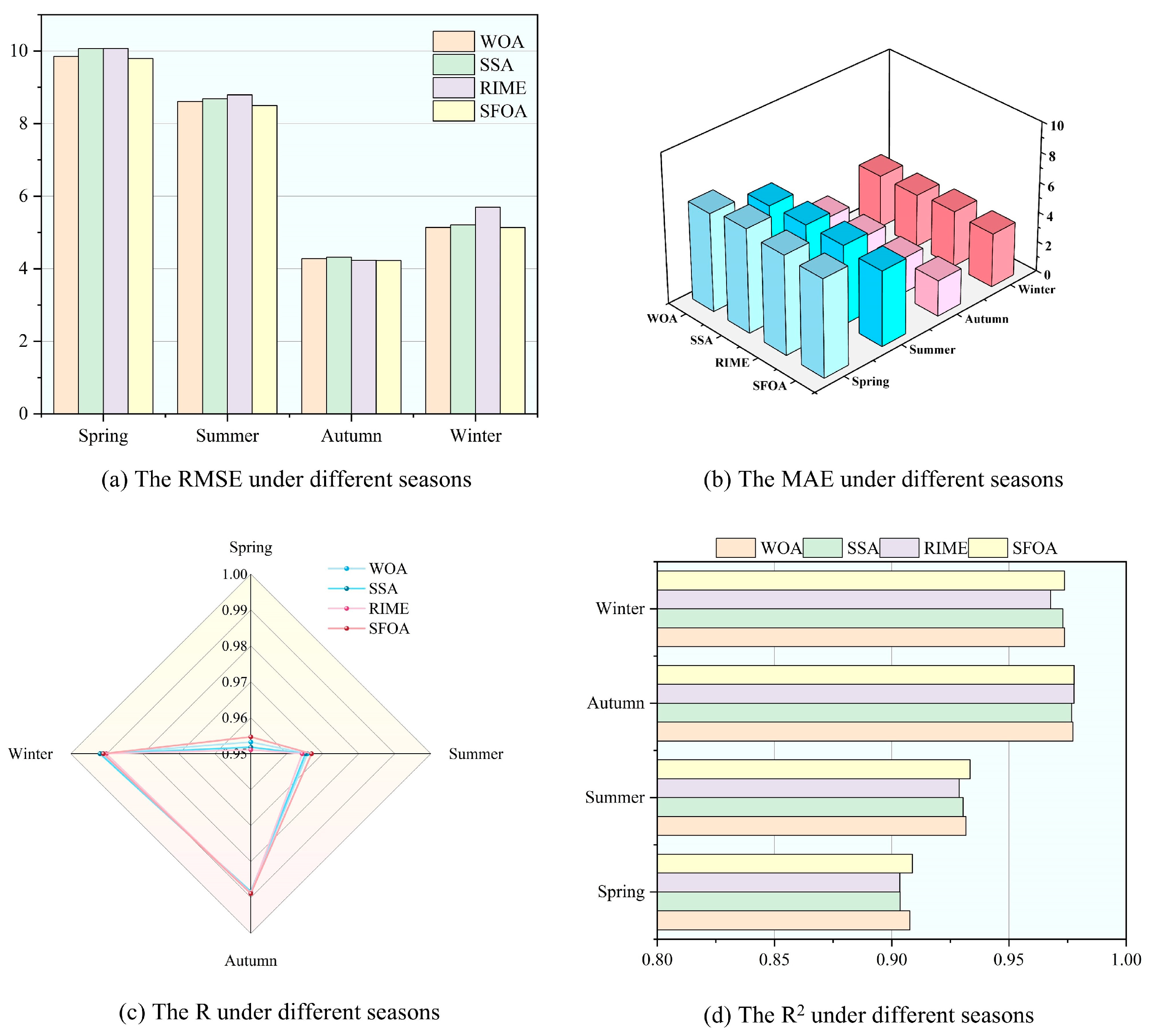
To validate the generalizability of the model, we extended the experiment by using an additional dataset sourced from a 1.8 MW distributed solar PV plant located in Uluru (Ayers Rock), Central Australia. Specifically, we selected Yulara Solar Site-2, which is equipped with a 226.8 kW polycrystalline silicon system, and analyzed data collected from 1 December 2017, to 30 November 2018 [24]. The data was divided into four seasons: Spring, Summer, Autumn, and Winter. The experimental procedure and related parameters remained consistent with the previous setup. First, the PCC was calculated, followed by EMD for denoising, and KPCA for feature dimensionality reduction. Subsequently, the four optimization algorithms were applied for training and prediction. Figure 10 presents the results of the experiment.

The results show that SFOA demonstrates excellent predictive capability on the new dataset as well. In the comparison across the four seasons, SFOA remains the overall leader. Although in Winter, SFOA’s MAE (3.589) is slightly higher than WOA (3.532) and SSA (3.530), and R (0.991) is slightly smaller than SSA (0.992), other metrics still outperform those of the other algorithms. In summary, SFOA consistently maintains low errors and high accuracy across different climatic conditions in all seasons, demonstrating its robust performance.

Furthermore, to assess the computational cost of each optimization algorithm, we measured the time taken for each algorithm to complete one optimization iteration. In all experiments, the population size was set to 10, and the number of iterations was set to 10, with each optimization algorithm successfully converging. According to the data in

Table 9. Time per iteration of optimization algorithms in different seasons.

Time Per Iteration (s)	Spring	Summer	Autumn	Winter
WOA	387.39	267.39	389.56	380.54
SSA	394.18	326.58	462.82	429.7.5
RIME	333.10	228.77	342.31	368.83
SFOA	332.82	266.72	341.37	377.20

, SFOA outperforms WOA and SSA in terms of optimization iteration time, while its computational time remains comparable to that of RIME. These findings demonstrate that, while improving prediction accuracy, SFOA does not significantly increase computational resource overhead, indicating a good balance between accuracy enhancement and computational efficiency.

6. Conclusions

To accurately predict PV power generation, this research introduces a short-term PV power prediction approach according to multi-method data processing and a CNN-BiLSTM model optimized by the SFOA. Initially, typical days are clustered using the K-means algorithm. Subsequently, key components are retained and redundant information is eliminated through the EMD and KPCA. Finally, a hybrid SFOA-CNN-BiLSTM model is developed to achieve accurate PV power prediction. The advantage of the proposed method is verified and analyzed through relevant case studies, leading to the following conclusions:

(1)

Combining EMD and KPCA to preprocess the input data enables the model to effectively filter out noise and irrelevant information. This process enhances the model’s ability to capture the underlying patterns and trends in the data, leading to more accurate and reliable predictions. Under three different scenarios, the RMSEs of the models processed with EMD-KPCA were reduced by 4.67%, 2.91%, and 2.67%, respectively, compared to those without it. The results illustrate the effectiveness of EMD-KPCA in improving the accuracy of PV data processing.

(2)

The SFOA-CNN-BiLSTM power prediction model can help to solve the problem of difficult parameterization of traditional deep learning networks and improve prediction accuracy. Compared to the model without SFOA, all metrics have improved dramatically. At the same time, compared with other optimization algorithms, SFOA has improved in most of the metrics and has the most comprehensive performance.

(3)

The proposed hybrid model outperforms other comparative models in most metrics, while also maintaining a low computational cost, thus demonstrating strong robustness and generalizability.

The hybrid model proposed in this paper can achieve good results in predicting PV power. However, there are still some shortcomings:

(1)

In this study, Pearson correlation was used to calculate and select relevant features. However, relying solely on Pearson correlation may overlook nonlinear and lagged relationships. In future research, we will pay more attention to selecting these types of features to improve the model’s performance and capture more complex dependencies.

(2)

Optimizing the hyperparameters of the network by using SFOA can significantly improve prediction accuracy. However, it has some weaknesses that may lead to suboptimal results, particularly in scenarios involving small real values, where relative errors have a greater impact. As a result, this can lead to a slightly higher MAPE compared to other algorithms, despite maintaining strong overall prediction accuracy. To address this issue, we will improve the SFOA in the next phase, or adopt more robust evaluation metrics and explore incorporating weighted error indicators or other techniques during the training process to mitigate bias in low-power regions, further enhancing the model’s accuracy and robustness.

(3)

The model currently relies solely on data-driven methods, without accounting for real-time physical mechanisms. Incorporating factors like irradiance, module temperature, and cloud dynamics could enhance the model’s credibility and transferability in real-world settings. These physical variables directly impact system performance and would improve the model’s robustness, making it more applicable in dynamic environments. Future work will explore integrating these physical elements to strengthen the model’s real-world accuracy.

References

1. Kakran, S.; Rathore, J.S.; Sidhu, A.; Kumar, A. Solar Energy Advances and CO2 Emissions: A Comparative Review of Leading Nations’ Path to Sustainable Future. J. Clean. Prod. 2024, 475, 143598. [Google Scholar] [CrossRef]
2. Maghami, M.R.; Hizam, H.; Gomes, C.; Radzi, M.A.; Rezadad, M.I.; Hajighorbani, S. Power Loss Due to Soiling on Solar Panel: A Review. Renew. Sustain. Energy Rev. 2016, 59, 1307–1316. [Google Scholar] [CrossRef]
3. Jiang, M.; Ding, K.; Chen, X.; Cui, L.; Zhang, J.; Yang, Z.; Cang, Y.; Cao, S. Research on Time-Series Based and Similarity Search Based Methods for PV Power Prediction. Energy Convers. Manag. 2024, 308, 118391. [Google Scholar] [CrossRef]
4. Massidda, L.; Bettio, F.; Marrocu, M. Probabilistic Day-Ahead Prediction of PV Generation. A Comparative Analysis of Forecasting Methodologies and of the Factors Influencing Accuracy. Sol. Energy 2024, 271, 112422. [Google Scholar] [CrossRef]
5. de Oliveira Santos, L.; AlSkaif, T.; Barroso, G.C.; de Carvalho, P.C.M. Photovoltaic Power Estimation and Forecast Models Integrating Physics and Machine Learning: A Review on Hybrid Techniques. Sol. Energy 2024, 284, 113044. [Google Scholar] [CrossRef]
6. Ferbar Tratar, L.; Strmčnik, E. The Comparison of Holt–Winters Method and Multiple Regression Method: A Case Study. Energy 2016, 109, 266–276. [Google Scholar] [CrossRef]
7. Rigby, A.; Baker, U.; Lindley, B.; Wagner, M. Generation and Validation of Comprehensive Synthetic Weather Histories Using Auto-Regressive Moving-Average Models. Renew. Energy 2024, 224, 120157. [Google Scholar] [CrossRef]
8. Shadab, A.; Ahmad, S.; Said, S. Spatial Forecasting of Solar Radiation Using ARIMA Model. Remote Sens. Appl. Soc. Environ. 2020, 20, 100427. [Google Scholar] [CrossRef]
9. Khan, Z.A.; Hussain, T.; Baik, S.W. Dual Stream Network with Attention Mechanism for Photovoltaic Power Forecasting. Appl. Energy 2023, 338, 120916. [Google Scholar] [CrossRef]
10. Wang, H.; Yi, H.; Peng, J.; Wang, G.; Liu, Y.; Jiang, H.; Liu, W. Deterministic and Probabilistic Forecasting of Photovoltaic Power Based on Deep Convolutional Neural Network. Energy Convers. Manag. 2017, 153, 409–422. [Google Scholar] [CrossRef]
11. Nhat, N.N.V.; Huu, D.N.; Nguyen, T.T.H. Short-Term Multi-Step Forecasting of Rooftop Solar Power Generation Using a Combined Data Decomposition and Deep Learning Model of EEMD-GRU. J. Renew. Sustain. Energy 2024, 16, 016101. [Google Scholar] [CrossRef]
12. Luo, X.; Zhang, D.; Zhu, X. Deep Learning Based Forecasting of Photovoltaic Power Generation by Incorporating Domain Knowledge. Energy 2021, 225, 120240. [Google Scholar] [CrossRef]
13. Zang, H.; Liu, L.; Sun, L.; Cheng, L.; Wei, Z.; Sun, G. Short-Term Global Horizontal Irradiance Forecasting Based on a Hybrid CNN-LSTM Model with Spatiotemporal Correlations. Renew. Energy 2020, 160, 26–41. [Google Scholar] [CrossRef]
14. Limouni, T.; Yaagoubi, R.; Bouziane, K.; Guissi, K.; Baali, E.H. Accurate One Step and Multistep Forecasting of Very Short-Term PV Power Using LSTM-TCN Model. Renew. Energy 2023, 205, 1010–1024. [Google Scholar] [CrossRef]
15. Li, Y.; Liu, G.; Cao, Y.; Chen, J.; Gang, X.; Tang, J. WNPS-LSTM-Informer: A Hybrid Stacking Model for Medium-Term Photovoltaic Power Forecasting with Ranked Feature Selection. Renew. Energy 2025, 244, 122687. [Google Scholar] [CrossRef]
16. Hou, Z.; Zhang, Y.; Liu, Q.; Ye, X. A Hybrid Machine Learning Forecasting Model for Photovoltaic Power. Energy Rep. 2024, 11, 5125–5138. [Google Scholar] [CrossRef]
17. Li, Y.; Huang, W.; Lou, K.; Zhang, X.; Wan, Q. Short-Term PV Power Prediction Based on Meteorological Similarity Days and SSA-BiLSTM. Syst. Soft Comput. 2024, 6, 200084. [Google Scholar] [CrossRef]
18. Zhou, D.; Liu, Y.; Wang, X.; Wang, F.; Jia, Y. Combined Ultra-Short-Term Photovoltaic Power Prediction Based on CEEMDAN Decomposition and RIME Optimized AM-TCN-BiLSTM. Energy 2025, 318, 134847. [Google Scholar] [CrossRef]
19. Zhang, J.; Sun, T.; Guo, X.; Lu, M. Short-Term Photovoltaic Power Prediction with CPO-BILSTM Based on Quadratic Decomposition. Electr. Power Syst. Res. 2025, 243, 111511. [Google Scholar] [CrossRef]
20. Wang, Z.; Ying, Y.; Kou, L.; Ke, W.; Wan, J.; Yu, Z.; Liu, H.; Zhang, F. Ultra-Short-Term Offshore Wind Power Prediction Based on PCA-SSA-VMD and BiLSTM. Sensors 2024, 24, 444. [Google Scholar] [CrossRef]
21. Zhang, Z.; Deng, A.; Wang, Z.; Li, J.; Zhao, H.; Yang, X. Wind Power Prediction Based on EMD-KPCA-BiLSTM-ATT Model. Energies 2024, 17, 2568. [Google Scholar] [CrossRef]
22. Peng, S.; Zhu, J.; Wu, T.; Yuan, C.; Cang, J.; Zhang, K.; Pecht, M. Prediction of Wind and PV Power by Fusing the Multi-Stage Feature Extraction and a PSO-BiLSTM Model. Energy 2024, 298, 131345. [Google Scholar] [CrossRef]
23. Zhong, C.; Li, G.; Meng, Z.; Li, H.; Yildiz, A.R.; Mirjalili, S. Starfish Optimization Algorithm (SFOA): A Bio-Inspired Metaheuristic Algorithm for Global Optimization Compared with 100 Optimizers. Neural Comput. Applic. 2025, 37, 3641–3683. [Google Scholar] [CrossRef]
24. DKA Solar Centre. Available online: https://dkasolarcentre.com.au/source/yulara/yulara-2-fixed-service-station (accessed on 11 May 2025).
Figure 1. The structure of the CNN-BiLSTM neural network model.
Energies 18 05124 g001
Figure 2. Schematic diagram of the SFOA-CNN-BiLSTM process.
Energies 18 05124 g002
Figure 3. General framework of PV power prediction method.
Energies 18 05124 g003
Figure 4. Clustering data graph of similar days: (a) strong sunlight and sunny weather; (b) moderate sunlight and cloudy weather; and (c) weak sunlight and rainy weather.
Energies 18 05124 g004
Figure 5. IMFs of each feature after EMD: (a) Total Radiation; (b) Direct Radiation; (c) Scattered Radiation; and (d) Component Temperature.
Energies 18 05124 g005
Figure 6. Chart of contribution rate distribution: (a) Scenario I; (b) Scenario II; and (c) Scenario III.
Energies 18 05124 g006
Figure 7. Forecast results for a typical day by using different models: (a) Scenario I; (b) Scenario II; and (c) Scenario III.
Energies 18 05124 g007
Figure 8. Forecast results for a typical day by using different methods: (a) Scenario I; (b) Scenario II; and (c) Scenario III.
Energies 18 05124 g008
Figure 9. Global comparison of model performance across three scenarios.
Energies 18 05124 g009
Figure 10. Key performance metrics comparison for the extended experiment.
Energies 18 05124 g010