Assessing the Technical and Economic Viability of Onshore and Offshore Wind Energy in Pakistan Through a Data-Driven Machine Learning and Deep Learning Approach

Abstract

An accurate estimation of wind energy productivity is crucial for the success of energy transition strategies in developing countries such as Pakistan, for which the deployment of renewables is essential. This study investigates the use of machine learning and deep learning techniques to improve wind farm producibility assessments, tailored to the Pakistani context. SCADA data from a wind turbine in Türkiye were used to train and validate five predictive models. Among these, Random Forest proved most reliable, attaining a coefficient of determination of 0.97 on the testing dataset. The trained model was then employed to simulate the annual production of a 5 × 5 wind farm at two representative sites in Pakistan—one onshore and one offshore—that had been selected using ERA5 reanalysis data. In comparison with conventional estimates based on the theoretical power curve, the machine learning-based approach resulted in net energy predictions up to 20% lower. This is attributable to real-world effects such as wake and grid losses. The onshore site yielded an LCOE of 0.059 USD/kWh, closely aligning with the IRENA’s 2024 national average of approximately 0.06 USD/kWh, thereby confirming the reliability of the estimates. In contrast, the offshore site exhibited an LCOE of 0.120 USD/kWh, thus underscoring the need for incentives to support offshore development in Pakistan’s renewable energy strategy.

1. Introduction

The 21st century will be pivotal in addressing the challenges of climate change [1]. The energy sector is responsible for approximately 38 Gt of CO₂ emissions [2], and it is thus a key area for intervention [3]. A transition to an energy mix dominated by renewables is imperative [4], as renewables are crucial not only for achieving climate neutrality but also for ensuring long-term energy security [5].

In recent decades there has been a significant rise in the use of renewable energy sources [6], driven by decreasing costs, technological advancements, and economies of scale. According to IRENA, the global average Levelized Cost Of Energy (LCOE) decreased to 0.034 USD/kWh and 0.079 USD/kWh in 2024, for onshore and offshore, respectively [7], thereby making it more competitive than fossil fuels in many regions worldwide. However, this transition is not uniform [8], with countries such as Pakistan in the Global South still exhibiting a pronounced gap between their technical potential and actual deployment [9].

Pakistan is one of the most vulnerable nations to the effects of climate change [10], as it consistently ranks in the top ten on the global Climate Risk Index [11]. Despite this, the national energy mix remains predominantly reliant on fossil fuels [9], with renewables (excluding hydropower) accounting for only 6.8% of installed capacity [12]. This 6.8% is primarily composed of wind (1850 MW), solar (680 MW), and bagasse (259 MW). At the same time, the inefficiencies of the national electricity system (with transmission and distribution losses higher than 18%) contribute to the exacerbation of national energy security [13].

The potential for renewable energy in Pakistan is significant [9]. The wind potential in the region is estimated to be over 340 GW [14], with the highest concentrations observed in the southern regions of Sindh and Baluchistan [15]. To date, however, the development of wind power projects has still been confined to onshore initiatives within the Gharo–Keti Bandar corridor area [14]. Despite favourable wind conditions along the Arabian Sea coast and the vast Exclusive Economic Zone (EEZ) [16], offshore wind energy remains unexplored in this region. This is particularly notable given the advantages of offshore wind [17], including usually higher capacity factors, greater predictability, and fewer land use conflicts compared to onshore installations.

Several key factors hinder the advancement of renewable energy sources in Pakistan, including [13]: the lack of a regulatory framework for offshore wind energy, the perception of high risk by financial institutions, the low benchmark tariffs set by National Electric Power Regulatory Authority (NEPRA), which is 0.046 USD/kWh for wind, the country’s reliance on imports (which introduces currency risks and customs duties), and the inadequacy of existing grid infrastructure.

Nonetheless, renewable energy remains central to Pakistan’s national strategies [18]. The Indicative Generation Capacity Expansion Plan (IGCEP) 2024-34 [19] projects significant growth in renewable energy, with an objective of 10% of the generation mix being derived from renewable energy by 2034. In parallel, the National Electricity Plan 2023–2027 [20] and the market reform (Competitive Trading Bilateral Contract Market, CTBCM [21]) aim to promote transparency, competitive auctions, and distributed generation.

While Pakistan’s energy policies place significant emphasis on the expansion of renewable energy sources, current assessments of wind energy potential remain limited in both methodology and accuracy. Although recent studies have demonstrated the effectiveness of ML and DL techniques for wind power potential estimation [22,23,24], in the Pakistani context to the best of our knowledge most previous studies have relied on theoretical power curves [25,26], neglecting the variability of real turbine operation under local conditions. At the same time, economic evaluations of wind power projects in Pakistan have been conducted using simplified assumptions [27], without integrating technical performance modelling into the LCOE framework.

In this context, the present study introduces a novel data-driven approach. For the first time, Machine Learning (ML) and Deep Learning (DL) models trained on real SCADA data from an operational wind turbine in Türkiye [28] are transferred and applied to meteorological data from Pakistan. This data-driven approach allows for the estimation of hourly wind power production potential in areas lacking long-term operational datasets, thus overcoming one of the major barriers to renewable energy planning in the region.

Furthermore, the study couples these data-driven performance models with comparative analysis of project profitability based on the LCOE [29]. This includes the integration of seabed depth constraints, cable lengths, and distance from the shore, all of which are key factors for offshore project planning.

This combined technical–economic framework aims to fill a double gap in the literature:

• the lack of ML/DL-based wind power modelling in Pakistan, and
• the absence of integrated economic assessments for both onshore and offshore sites.

The study aims to assess whether the physical and economic conditions in selected coastal and offshore areas of Pakistan are favourable to large-scale wind energy deployment. The findings of this study can serve as a basis for investment decisions, regulatory updates, and climate fund allocation, helping to close the gap to internationally agreed sustainability targets.

2. Methods and Data

This section describes the methods used to estimate the energy producibility of wind turbines through theoretical power curves and ML and DL models. The main predictive models, performance evaluation metrics, and the analysis of energy losses due to wake effects and grid losses are introduced. Then, the economic approach taken to assess project sustainability is presented, with the calculation of CAPEX, OPEX, and LCOE costs. Finally, the operational dataset of an onshore wind turbine located in Yalova, Türkiye, used for training the ML and DL models is presented.

2.1. Producibility of a Wind Turbine

The estimation of the energy producibility of a wind turbine is a fundamental step in the feasibility assessment of renewable energy projects. This section delineates the adopted technical methodology to estimate energy production from wind, based on theoretical models (power curves) and machine learning-based approaches. Furthermore, performance indicators such as the capacity factor and statistical metrics used to evaluate model accuracy are introduced.

2.1.1. Power Curve

The theoretical power output of a wind turbine can be estimated using the following equation, which describes the nonlinear relationship between wind speed at hub height and available wind power [30]:

$$P_m={\displaystyle \frac{1}{2\cdot 1000}}\rho A{V}^3{C}_p(\lambda ,\alpha )$$

(1)

where $P_m$ [kW] is the mechanical power generated by the wind turbine, $\rho$ [kg/m³] the air density, $A$ [m²] the swept area, $V$ [m/s] the wind speed, $C_p$ [-] the power coefficient, $\lambda$ [-] the tip speed ratio, and $\alpha$ [°] the pitch angle.

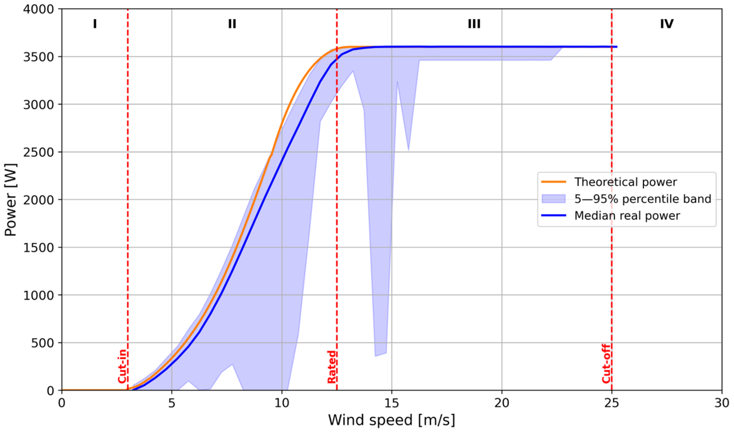
Although the fundamental power equation is based on physical principles and provides an idealised estimate of available wind power, the turbine’s power curve is derived empirically from operational data. This curve more accurately reflects the turbine’s actual performance, including operational limits and control mechanisms, and thus provides a more realistic estimation of power output. As shown in Figure 1, the graph of a power curve can be divided into four distinct regions, each defined by three velocities:

• The region below the cut-in speed $V_{cut-in}$, that is, the minimum wind speed at which the turbine starts generating power.
• The region where the power output varies in proportion to the cube of speed, which extends from the cut-in speed $V_{cut-in}$ to the rated speed $V_{rated}$.
• The rated power region, beyond the rated speed $V_{rated}$, is the region in which the turbine produces its maximum constant power output. The turbine operates at rated power throughout this region, until the cut-off speed $V_{cut-off}$ is reached.
• The region above the cut-off speed $V_{cut-off}$ of the turbine, after which the turbine is stopped to prevent mechanical or structural damage.

Figure 1. The power curve of a wind turbine divided into the four regions delineated by the cut-in, rated, and cut-off wind speeds.

Figure 1. The power curve of a wind turbine divided into the four regions delineated by the cut-in, rated, and cut-off wind speeds.

The power curve is a crucial component in the design of wind farms, as it enables the estimation of the producibility of a chosen location. This can be achieved by using data collected during a wind measurement campaign or with satellite meteorological data. However, using theoretical power curves calibrated through the IEC standard procedure [31] (reference air density ${\rho }_{ref}=1.225$ kg/m³ at sea level) can lead to errors of overestimation as the curves neglect the consideration of real environmental variables such as air density, turbulence, and turbine degradation.

2.1.2. Machine Learning and Deep Learning Models for Wind Power Prediction

ML ad DL models are increasingly used to enhance the precision of producibility estimates. Unlike static power curves, ML and DL models can learn nonlinear relationships between wind speed and actual energy production, incorporating a variety of environmental features.

In this study, an historical dataset combining meteorological variables with theoretical and observed energy output was used to train predictive models. The tested ML and DL models are commonly used in wind power prediction studies [32,33,34,35,36,37] and represent diverse algorithmic families, enabling a comprehensive evaluation of predictive performance across tree-based and neural network approaches. The chosen ML and DL models are the following:

• Gradient Boosting (GBoost) [38]: GBoost is a ML model that employs decision trees as weak learners, combining them sequentially to form a strong learner (Figure 2a). This process ensures a more accurate model by progressively reducing errors from previous iterations. Moreover, GBoost utilises residual errors as weight values and optimise the classification performance by using adjustable learning rates and loss functions. However, adding trees sequentially can slow down the learning process when dealing with large datasets.
• Extreme Gradient Boosting (XGBoost) [39]: XGBoost is the advanced version of GBoost, with refinements such as integrating regularisation (L1, L2) [40] by adding a penalty term to the loss function, the computation of second derivatives of the loss function, and parallel optimisation. This combination of characteristics enhances the model’s efficiency and reduces the risk of overfitting.
• Random Forest (RF) [41]: RF is an ensemble learning algorithm based on parallel training with multiple decision trees (Figure 2b). In the training phase of the algorithm, multiple trees are constructed, with each tree being built on a random sample of the dataset. The prediction made by each tree is then averaged. In RF, the number of trees and their depths are higher than those in GBoost and XGBoost. RF demonstrates efficacy in the presence of noisy or highly nonlinear data, such as hourly weather data, because of its robustness and capacity for generalisation.
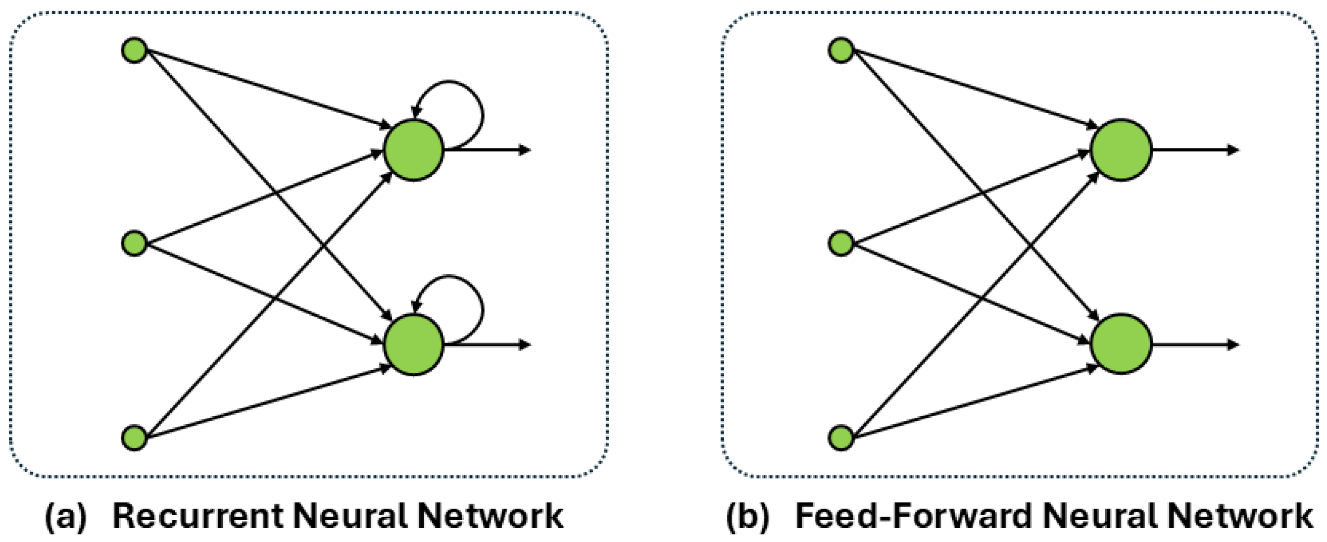
• Multi-Layer Perceptron (MLP) [40]: MLP constitutes the primary DL architecture. It is a feed-forward neural network (Figure 3a) consisting of one or more hidden layers with nonlinear activation functions. Although MLP is capable of modelling complex relationships between inputs and outputs, it does not account for the temporal component in the data, thus limiting its effectiveness in time series analysis.
• Long Short-Term Memory (LSTM) [40]: LSTM is a recurrent neural network architecture employed in the context of DL. In contradistinction to conventional feed-forward neural networks, such as MLP, LSTM employs feedback links (Figure 3b). LSTM networks find application in the analysis and learning of sequential data. Consequently, LSTM networks are a suitable option for data that follows a sequential format.

The dataset is divided into a training set (80%) and a test set (20%) in order to evaluate the performance of ML and DL models. For the non-sequential models (namely: RF, XGBoost, GBoost, and MLP), the division is conducted randomly. In contrast, the LSTM model requires preservation of the temporal sequence, and thus the split is performed while maintaining the chronological order of the data.

An optimisation by genetic algorithm is then conducted for each ML or DL algorithm to identify the optimal parameters associated with each, leveraging the Python (version 3.11) DEAP library. Specifically, 10 generations of 30 individuals are selected, with an elitism of 3 individuals.

2.1.3. Energy Performance

The Capacity Factor (CF) is a key metric employed to assess the energy performance of wind turbines. It is defined as the ratio of the energy produced $E_{produced}$ in a given period of time $t$, usually a year, to the maximum energy theoretically producible if the turbine operated at its rated power $P_{nom}$ for the entire duration of the period under consideration [42]:

$$\mathrm{CF}={\displaystyle \frac{E_{produced}}{P_{nom}\cdot t}}$$

(2)

This index is particularly useful for comparing different turbines or evaluating the performance of the same turbine under different environmental conditions.

2.1.4. Metrics

In order to assess a model accuracy, a comparison is made between the actual active power values of the dataset and the model’s predicted active power output values. The Mean Absolute Error (MAE) [43], Root Mean Squared Error (RMSE) [44], and the Coefficient of Determination ${\mathrm{R}}^2$ [45] are used, which are defined as follows:

$$\mathrm{MAE}={\displaystyle \frac{1}{n}}{\displaystyle \sum _{i=1}^n|y_i-{\stackrel{⌢}{y}}_i|}$$

(3)

$$\mathrm{RMSE}=\sqrt{{\displaystyle \frac{1}{n}}{\displaystyle \sum _{i=1}^n{(y_i-{\stackrel{⌢}{y}}_i)}^2}}$$

(4)

$${\mathrm{R}}^2=1-{\displaystyle \frac{{\displaystyle \sum _{i=1}^n{(y_i-{\stackrel{⌢}{y}}_i)}^2}}{{\displaystyle \sum _{i=1}^n{(y_i-{\overline{y}}_i)}^2}}}$$

(5)

where $y_i$ is the active power output from the dataset, ${\stackrel{⌢}{y}}_i$ the model’s predicted active power output, ${\overline{y}}_i$ the mean value of the active power outputs from the dataset, and $n$ the total number of outputs.

2.2. Energy Losses

Within the context of wind energy generation, wind turbines situated within a wind farm are susceptible to various forms of energy loss. These losses can be attributed to two primary factors: the configuration of the wind farm, specifically the spacing between turbines, and the distance from the substation.

2.2.1. Wake Losses

Energy losses associated with the wake effect represent a significant factor in the design of wind farms, particularly in configurations with high turbine density. The extraction of energy from the wind by a turbine results in the generation of a turbulent wake downstream, characterised by a reduction in flow velocity and an increase in turbulence intensity [46]. Consequently, turbines situated within this wake receive a reduced airflow of lower energy intensity, thereby diminishing the potential power output. The extent of this loss is therefore a function of the relative distance between the wind turbines and can be taken into consideration using the unit efficiency.

Table 1. Single wind turbine efficiency [%] as a function of turbine spacing [D = rotor diameters] and wind farm array size [N × N].

Turbine Spacing [D = Rotor Diameters]	5 × 5	10 × 10	50 × 50
5	85%	70%	29%
9	94%	86%	62%
16	98%	96%	87%
28	99%	98%	95%

shows turbine efficiency for wake losses values known in the literature [47] as a function of turbine spacing for three different array size of wind farms.

As the distance between turbines increases, an increase in the unit efficiency is observed, indicating a reduction in the influence of the unit efficiency and, thus, a decrease in overall power losses. Moreover, the larger the array, the lower the unit efficiency since there is a lower replenishment of wind kinetic energy that will reach the next unit of the array.

2.2.2. Grid Losses

Grid losses occur when electric power is transmitted from wind turbines to the substation on the ground [46]. These losses encompass those attributable to transformers, converters, and cable resistance. The distance between the generators and the substation is a key factor, since the length of the cables directly correlates to the resistive losses.

A comparison of High-Voltage Alternating Current (HVAC) and High-Voltage Direct Current (HVDC) connections shows that DC systems exhibit higher initial losses due to AC/DC conversion. However, these systems demonstrate greater efficiency over long distances due to lower losses along the cables. Consequently, a threshold distance is identified (Figure 4) beyond which DC transmission becomes more economically advantageous than AC.

The estimation of grid losses is conducted according to [46] as follows:

$${\mathrm{HVAC}}_{\mathrm{losses}}=1.79\cdot {10}^{-6}\cdot f^2+2.28\cdot {10}^{-5}\cdot f+1.68\cdot {10}^{-2}$$

(6)

$${\mathrm{HVDC}}_{\mathrm{losses}}=2.26\cdot {10}^{-5}\cdot f+3.42\cdot {10}^{-2}$$

(7)

where $f$ [km] is the distance to the substation.

2.3. Economic Analysis

The assessment of sustainability and profitability of wind energy projects requires economic analysis as a fundamental step. This section examines the main economic components that determine the total cost of energy production. Following a thorough examination of the capital expenditures (CAPEX) and annual operating expenditures (OPEX) associated with both onshore and offshore facilities, the constant currency approach is outlined to ensure the uniformity of economic estimations over the course of time. Finally, the LCOE is calculated, a key indicator for comparing the economic efficiency of the project with other generation technologies.

2.3.1. CAPEX and OPEX

CAPEX refers to the initial investment costs, which include the costs of the turbine, foundation, installation and grid connection [48]. CAPEX varies depending on whether the wind farm is located onshore or offshore.

For an onshore turbine, the following cost components are identified as follows [49]:

• Turbine: 1064 EUR₂₀₂₀/kW
• Foundation: 69 EUR₂₀₂₀/kW
• Other (grid connection and installation): 192 EUR₂₀₂₀/kW

For an offshore turbine, on the other hand, CAPEX costs are generally higher and broken down as follows:

• Turbine [49]: 1215 EUR₂₀₂₀/kW
• Foundation: The choice of the type of foundation is dictated by the depth of the seabed $d$. In very shallow waters (<25 m) the monopile is preferred, whereas for intermediate to deep waters (25–55 m), jacket foundations are more suitable. Estimated costs in USD₂₀₁₆/kW are [50]:

  ○

  Monopile:

  $${\mathrm{CAPEX}}_{\mathrm{monopile}}=\left(201\cdot d^2+612.93\cdot d+411464\right)\cdot {\displaystyle \frac{1}{1000}}$$

  (8)

  ○

  Jacket:

  $${\mathrm{CAPEX}}_{\mathrm{jacket}}=\left(114.24\cdot d^2-2270\cdot d+531783\right)\cdot {\displaystyle \frac{1}{1000}}$$

  (9)

• Installation: Offshore installation is more complex and costly due to the need for specialised vessels and weather constraints. The cost for the installation [48] is estimated in USD₂₀₁₆m as:

$${\displaystyle \frac{\left[\left(day{s}_{install}+day{s}_{to-site}\right)\cdot cos{t}_{jack-up}+lengt{h}_{cable}\cdot cos{t}_{cable-install}\right]}{capacit{y}_{wind\hspace{0.17em}\hspace{0.17em}farm}}}$$

(10)

where $day{s}_{install}=2$ is the number of days needed to install each turbine, $day{s}_{to-site}$ the journey time as a function of the distance, $cos{t}_{jack-up}=0.25\hspace{0.17em}\hspace{0.17em}\mathrm{USDm}/\mathrm{day}$ the assumed vessel cost, $lengt{h}_{cable}$ the length of the cable, $cos{t}_{cable-install}=0.1\hspace{0.17em}\hspace{0.17em}\mathrm{USDm}/\mathrm{km}$ the assumed installation cost for the cables, $capacit{y}_{wind\hspace{0.17em}\hspace{0.17em}farm}$ the installed capacity of the wind farm. The $day{s}_{to-site}$ are estimated as follows:

$$day{s}_{to-site}=2\cdot \left({\displaystyle \frac{distance}{spee{d}_{jack-up}\cdot hour{s}_{working-day}\cdot N_{turb-per-visit}}}\right)$$

(11)

where $distance$ is the distance [km] to the coast, $spee{d}_{jack-up}=20\hspace{0.17em}\hspace{0.17em}\mathrm{km}/\mathrm{h}$ the average speed of the installation vessel, $hour{s}_{working-day}=24\hspace{0.17em}\hspace{0.17em}\mathrm{h}$ the length of the working day, $N_{turb-per-visit}=5$ the assumed number of turbines the installation vessel can carry per visit. The assumed costs and values are comparable to those documented in the existing literature [48].

• Grid: The cost of grid connection in offshore wind projects depends significantly on the transmission technology adopted, that is, HVAC or HVDC. Once again, HVAC is preferred for shorter distances due to its lower capital cost and simpler infrastructure. HVDC becomes more cost-effective for longer distances, as it minimises transmission losses and allows for more efficient long-distance power transfer, despite higher initial costs. The grid cost can be estimated in USD₂₀₁₉m/kW for the two case as follows [46]:

$${\mathrm{HVAC}}_{\cos \mathrm{t}}=\left(0.0085\cdot f+0.0568\right)\cdot {\displaystyle \frac{1}{1000}}$$

(12)

$${\mathrm{HVDC}}_{\cos \mathrm{t}}=\left(0.0022\cdot f+0.3878\right)\cdot {\displaystyle \frac{1}{1000}}$$

(13)

OPEX refers to costs associated with the ongoing Operation and Maintenance of a wind farm throughout its lifetime [49]. The costs encompass scheduled and unscheduled maintenance, monitoring, insurance, land or seabed lease fees, administrative expenses, and other recurring services necessary to ensure continuous operation of the facility. OPEX values are generally expressed as a percentage of the initial CAPEX [46], particularly in preliminary economic assessments.

In this analysis, the following assumptions have been adopted:

• Onshore OPEX: 1.5% of CAPEX, annually.
• Offshore OPEX: 2% of CAPEX, annually.

2.3.2. Constant Currency Approach

To ensure consistency and comparability of economic values over the lifetime of the project, all costs and revenues in this analysis are expressed in USD₂₀₂₄. When using cost data from sources in other currencies and reference years, a two-step adjustment is performed. For example, for EUR₂₀₂₀ the two-step adjustment comprises:

• Currency conversion to dollars using an average exchange rate for that year [51].
• Inflation adjustment to bring historical values to 2024 values using official inflation indices, using the annual average Consumer Price Index (CPI) [52] in the following equation:

$${\mathrm{Price}}_{\mathrm{YEAR} 2}{=\mathrm{Price}}_{\mathrm{YEAR} 1}\cdot {\displaystyle \frac{{\mathrm{CPI}}_{\mathrm{YEAR} 2}}{{\mathrm{CPI}}_{\mathrm{YEAR} 1}}}$$

(14)

The conversion rate used for the currency exchange from EUR₂₀₂₀ to USD₂₀₂₀ is 1.1422, while the CPIs used for the years 2016, 2020 and 2024 are 240, 258.8 and 313.7, respectively.

By adopting a constant currency approach, the LCOE reflects only technical and economic parameters, avoiding distortions caused by projected price level changes over time.

2.3.3. Levelized Cost Of Energy

The LCOE is defined as the average cost per unit of electricity generated over the lifetime of the project [46], expressed in USD₂₀₂₄. It is a key indicator for evaluating the economic competitiveness of energy generation technologies, as it incorporates CAPEX, OPEX, and energy production, discounted over time. The LCOE is calculated as follows [46]:

$$\mathrm{LCOE}={\displaystyle \frac{\mathrm{CAPEX}\cdot \mathrm{CRF}+\mathrm{OPEX}}{E_{annual}}}$$

(15)

where $E_{annual}$ is the annual energy production and $\mathrm{CRF}$ the Capital Recovery Factor, which can be calculated as:

$$\mathrm{CRF}={\displaystyle \frac{r\cdot {\left(1+r\right)}^n}{{\left(1+r\right)}^n-1}}$$

(16)

where $r$ is the Weighted Average Cost of Capital (WACC), which represents the average rate required by investors to finance the project [53]. Assuming a project lifetime of 25 years and a WACC of 5%, the corresponding $\mathrm{CRF}$ is:

$$\mathrm{CRF}={\displaystyle \frac{0.05\cdot {\left(1+0.05\right)}^{25}}{{\left(1+0.05\right)}^{25}-1}}\cong 0.0710$$

(17)

Thus, for each kW of installed capacity, the annualised capital cost is equivalent to approximately 7.1% of the total CAPEX. This annualised cost is then added to the OPEX and divided by the annual energy production to obtain the LCOE.

2.4. Türkiye SCADA Dataset

This section describes the Türkiye SCADA dataset employed for the training of the models, along with the preprocessing steps and model configuration used to ensure consistent and fair comparison of predictive performance.

2.4.1. Dataset Description

The operational dataset of an onshore wind turbine [54] located in Yalova, Türkiye (40.58545° N, 28.99035° E) [55] was utilised to train the ML and DL models. Figure 5 shows the geographical location of the wind farm from which the data for the selected turbine were obtained.

The plant has a total installed capacity of 32.4 MW and comprises 9 Nordex N117/3600 turbines [24], with a nominal power of 3.6 MW [56] for each turbine. The associated SCADA system records data at 10 min intervals for a single turbine over the course of the year 2018. The dataset under consideration contains 50,530 data points. A complete dataset for the year would consist of 52,560 points; thus, less than 3.9% of the data is missing. Such information may be absent due to device malfunction or other technical issues. In this study, incomplete data points were discarded without compromising the overall representativeness of the dataset, as their proportion is found to be relatively small.

The dataset under consideration includes the following variables: timestamp, wind speed [m/s] and direction [°] at hub height, theoretical power output [kW] calculated using the theoretical power curve, and actual active power output [kW].

The analysis of wind distribution from the wind rose in Figure 6 indicates that the predominant directions are east-northeast (ENE), northeast (NE) and south-southwest (SSW), with frequencies of 25.9%, 20.6% and 16.6%, respectively. The predominance of moderate speeds, ranging from 3 to 9 m/s, indicates that the wind conditions are generally stable and moderate. Winds with speeds greater than 15 m/s are extremely rare, with almost zero percent of all directions exhibiting such velocities. Directions such as east (E), east-southeast (ESE), southeast (SE), northwest (NW), and north-northwest (NNW) exhibit frequencies of less than 1%, suggesting that wind from these directions have negligible impact at the analysed site. In instances where wind directions exhibit low representativeness, the quality of forecasts may be diminished.

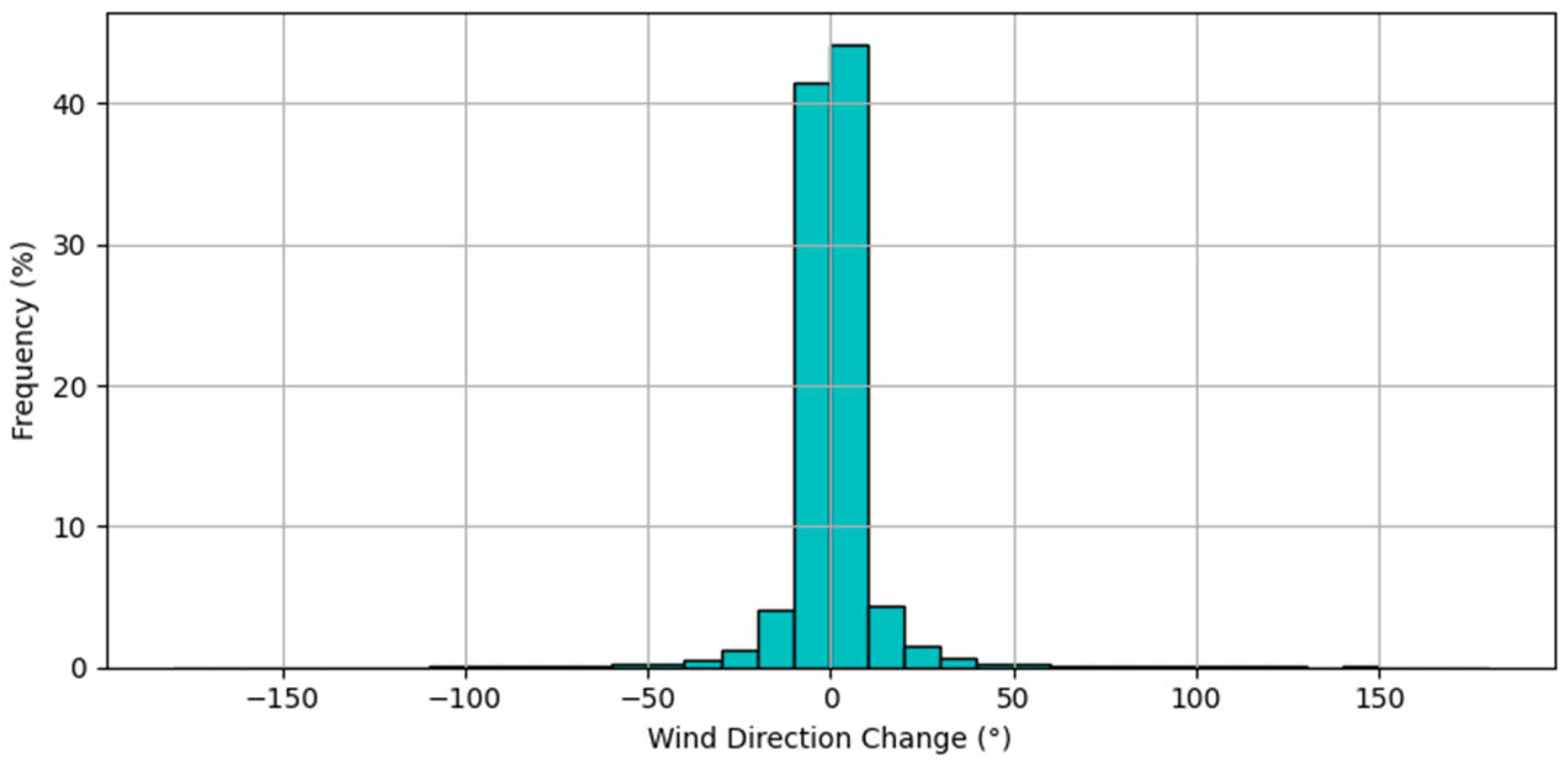
Figure 7 shows the distribution of wind direction changes (in degrees), expressed as percentages over the entire year of data acquisition. The data from Türkiye indicate that wind direction variability between consecutive measurements is generally low, with over 80% of changes below 10°. However, since the training data mainly consists of winds from two directions that exhibit limited variability, caution is needed if the trained model is to be used in significantly different climatic conditions.

In order to mitigate the potential for bias arising from site-specific prevailing directions, it should be noted that the absolute wind direction is not to be utilised as an input model when employing this dataset for the training phase. Consequently, in this work the models were trained on the variation in wind direction between consecutive datapoints rather than the absolute direction.

Since the SCADA data utilised in this study originates from a turbine that is part of a real wind farm comprising nine Nordex N117/3600 turbines, as a result, wake losses among turbines are already incorporated into the recorded power data. Consequently, ML and DL models trained on this dataset implicitly take these losses into account. Furthermore, since the SCADA dataset used for model training refers to an onshore turbine, offshore-specific variables (e.g., turbulence intensity, gusts, wave frequency and height) are not represented.

2.4.2. Preprocessing and Model Configuration

The training of the five ML and DL models was achieved through the utilisation of five Python codes. The following section outlines the primary steps involved in this process.

• Data loading: The dataset is uploaded using the pandas library, upon which the data points are sorted by timestamp and any duplicates are removed. Following this, rows with missing values (NaN) in the main columns (wind_speed, wind_direction, theoretical_power, active_power) are deleted. No imputation or masking is performed.
• Calculation of variations: This process entails the calculation of the differences between successive data points on wind speed, wind direction and theoretical power (i.e., the active power calculated via the theoretical power curve). The objective of this calculation is to obtain “d_wind_speed” [m/s], “d_wind_direction” [°] and “d_theoretical_power” [kW].
• Choosing the input features and output of interest: The input features for all the developed models are as follows: “d_wind_speed” [m/s], “d_wind_direction” [°], “d_theoretical_power” [kW], “theoretical_power” [kW], “wind_speed” [m/s]. The incorporation of variations between consecutive timestamps facilitates the capture of temporal dynamics in turbine changes, even for non-sequential models. The output of interest is always “active_power” [kW] for all five models. It is important to note that the present study omitted consideration of certain environmental variables, such as temperature, atmospheric pressure, and air density, due to the unavailability of these variables within the original dataset.
• Outliers removal: The elimination of outliers is achieved through the implementation of a Z-score filter on all features and targets, resulting in the removal of values that deviate by more than three standard deviations from the average value. The percentage of rows that are deleted as a consequence of missing values and outliers removal is 4.9% of the original dataset.
• Inputs standardisation: StandardScaler is utilised for the purpose of standardising the input features. Standardisation is a process that facilitates convergence, thereby ensuring the comparability of data across diverse models.
• Train/test split: The train/test split of the dataset is achieved by employing the train_test_split function, which is utilised across all models to randomly divide the dataset into an 80/20 ratio (80% for training, 20% for testing). In contrast to other models, LSTM employs a data split that is not random but rather follows the timeline, using the initial 80% of the data for training and the remaining 20% for testing, thereby ensuring temporal sequence is respected. Hence, LSTM is the only model that respects the temporal sequence, which is imperative for modelling temporal dependence. All other models treat the data as independent, meaning that the model does not directly capture temporal dependencies.
• Hyperparameter optimisation: the hyperparameters were optimised using a genetic approach (10 generations of 30 individuals), with the DEAP library and exploiting multiprocessing. The implementation of elitism equal to 3 in each of the models ensures the retention and carry-over of the three best individuals from the current generation to the next. Each individual is representative of a set of model hyperparameters, and the fitness function is R² on the complete dataset.

Adopting this preprocessing and configuration procedure ensures that all models are trained on standardised features, including absolute values of wind speed and theoretical power, as well as variations between consecutive time instants of wind speed, direction, and theoretical power, to reduce the risk of bias related to the source site. Such steps prepare the models for a transductive transfer learning approach [57], in which the knowledge acquired from the turbine data in Türkiye can be transferred to a new domain, such as meteorological data from Pakistan, without additional training.

3. Case Study

This section presents the climatic characterisation of the coastal region of Pakistan, influenced by summer monsoons, as well as the weather dataset for 2018, extracted from ERA5. Finally, the configuration of the wind farm later simulated at two sites in Pakistan is introduced.

3.1. Pakistan Climate

The coastal region of Pakistan’s EEZ is characterised by arid climatic conditions [58], influenced by the summer monsoon that typically extends from June to September [59]. During this season, winds from the Indian Ocean exhibit a significant increase in both speed and intensity. This phenomenon is attributed to the differential heating between land and sea, which results in the generation of stronger air currents than are observed during the rest of the year. The monsoon winds contribute to increase the atmospheric turbulence, thereby playing a crucial role in the variability of local wind power production. The intensification of summer winds [25] is a key factor in the development of renewable energy resources in the coastal region, rendering Pakistan a subject of particular interest for studies of offshore and coastal wind energy production.

3.2. Pakistan Data

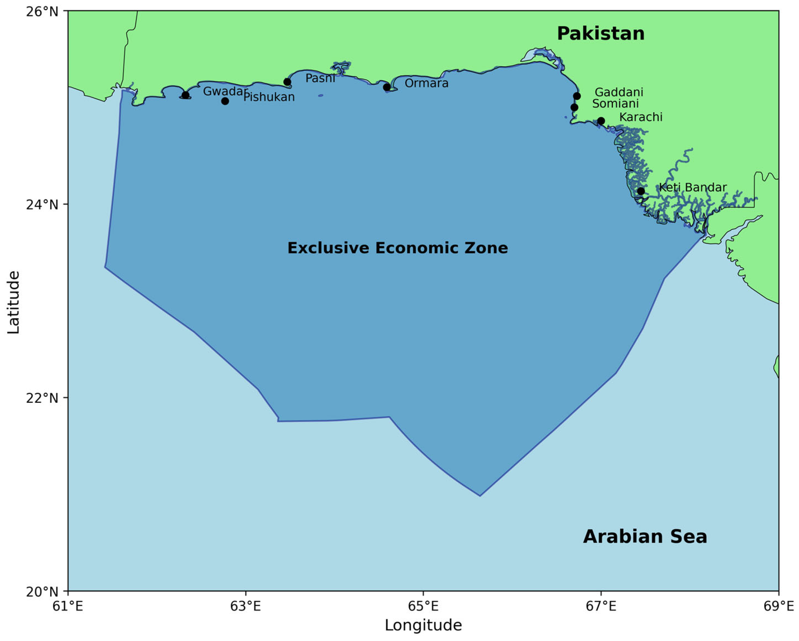
In order to extend the analysis to the Pakistani region, a set of meteorological data was extracted from the ERA5 reanalysis database [60]. This extracted dataset covers the entire year 2018 with hourly resolution. The selected spatial domain encompasses a grid of points with a spacing of 0.25° × 0.25°, delineated by the following geographical coordinates: North: 26° N, West: 61° E, South: 20° N, East: 69° E. This area encompasses the whole EEZ of Pakistan, as shown in Figure 8. The variables retrieved from ERA5 include the eastward $u$ and northward $v$ components of wind at 100 m, and the seabed depth $d$, for offshore suitability analysis.

The objective is to identify, using Python-based data processing code, two representative locations:

• The windiest onshore coastal site, characterised by the highest annual mean wind speed.
• The windiest offshore site with the shallowest seabed depth, to ensure the feasibility of foundation design.

For both selected locations, the wind components $u$ and $v$ are converted into wind intensity and wind direction variables, respectively. Then, hourly time series of wind speed at a hub height of 141 m are obtained by converting the wind intensity as follows, using the logarithmic wind profile law [61]:

$$V_{141}=V_{100}\cdot {\displaystyle \frac{\ln \left(\frac{141}{z_0}\right)}{\ln \left(\frac{100}{z_0}\right)}}$$

(18)

where $V_{141}$ and $V_{100}$ are the wind speed at 141 and 100 m, respectively, and $z_0$ the surface roughness length. The following values are assumed for roughness surface length: $z_0=0.0003\hspace{0.17em}\hspace{0.17em}\mathrm{m}$ for the offshore location [62], $z_0=0.03\hspace{0.17em}\hspace{0.17em}\mathrm{m}$ for the coastal location [63].

This approach allows to adjust the raw ERA5 data to the specific turbine height, considering the effect of surface roughness on the wind vertical profile.

3.3. Proposed Wind Farm

The proposed wind farm is composed of a 5 × 5 matrix of turbines, arranged with an inter-turbine distance of 7 times the rotor diameter. This configuration yields a wake efficiency of approximately 90%, as seen in Section 2.2.1. Although the ML and DL algorithm employed inherently incorporates wake losses, this data is utilised for the simulation using the power curve.

The turbine selected is the N117/3600 model, which is classified according to IEC standards as a class II turbine. It is characterised by a rotor diameter of 117 m and a rated power of 3.6 MW. Even though it is not specifically designed for offshore applications, it is used in this study because the ML and DL models were trained with data collected from this type of turbine. The primary technical characteristics of the device include a cut-in speed of 3 m/s, a rated speed of 12.5 m/s, and a cut-off speed of 25 m/s, enabling production in a wide range of wind conditions.

4. Results and Discussion

This section provides a detailed comparison between the Theoretical Power Curve and the Real Power Curve derived from the dataset. Subsequently, the optimisation results of the ML and DL models are presented, with the selection of the most appropriate model. Consequently, the utilisation of the selected model enables the estimation of producibility for two sites in Pakistan. Finally, the economic analysis provides an understanding of the different profitability of the assumed plant at the two different sites

4.1. Theoretical and Real Power Curves

Figure 9 presents a comparison between the measured active power values (blue band) and the corresponding theoretical values (in orange) of the Turkish SCADA dataset. Additionally, the curve representing the median of the recorded active power output values in the dataset is shown in blue. The theoretical values, calculated according to the power curve provided by the manufacturer as a function of wind speed, form the theoretical power curve of the turbine. It is in zone II of the theoretical power curve that the most significant deviation between the recorded and the theoretical data is observed. Within this operational range, the distribution of the measured points exhibits a significantly greater dispersion around the theoretical curve. Such discrepancies imply that real operating conditions, including aerodynamic losses, turbulence, and wake effects within the wind farm, significantly influence the energy performance of the turbine, resulting in a deviation from the theoretical prediction of the rated power.

The blue band in Figure 9 represents the 5th–95th percentile of the real power, reflecting the natural variability of the data. Wider sections of the blue band, such as those observed in zone III, can be attributed to the presence of outliers. Such outliers, which may be resulting from abnormal or transient operating conditions, were eliminated during the pre-processing stage to ensure the reliability of the predictive model training.

A comparison of real measured and theoretical data using the R², MAE and RMSE metrics revealed a reasonable degree of agreement, as shown in

Table 2. Metrics resulting from the comparison between real and theoretical power outputs.

Metrics	DATASET: True y = Active Power Predicted y = Theoretical Power
R2	0.879
MAE	192.76 W
RMSE	456.19 W

.

The R² value obtained by the comparison between the Real Power Curve and the Theoretical Power Curve is selected as the reference baseline. Therefore, the ML and DL algorithms developed in this study must demonstrate a performance that exceeds this value in order to be considered effective in improving the prediction of turbine producibility.

4.2. ML and DL Models Performance

The results of the ML and DL models optimisation are shown in

Table 3. Results of the optimisation of the ML and DL models studied.

Model	Optimal Parameters	R2 Test	R2 Total	MAE Test [kW]	MAE Total [kW]	RMSE Test [kW]	RMSE Total [kW]
GBoost	n_estimators = 292, learning_rate = 0.283, max_depth = 10, subsample = 0.791, min_samples_split = 2, min_samples_leaf = 1	0.884	0.975	197.923	71.484	444.682	206.315
XGBoost	n_estimators = 563, max_depth = 10, learning_rate = 0.189, subsample = 0.983, colsample_bytree = 0.978	0.884	0.976	197.732	54.843	447.061	202.255
RF	n_estimators = 556, max_depth = 35, min_samples_split = 2, min_samples_leaf = 1, max_features = 0.933	0.901	0.970	173.024	84.105	410.574	225.545
MLP	hidden_layer_size = 162, activation = tanh, alpha = 0.010, learning_rate = 0.038	0.907	0.916	160.319	153.178	398.563	380.120
LSTM	hidden_layer_size = 70, dropout = 0.009, rec_dropout = 0.137, learning_rate = 0.007	0.914	0.915	201.809	157.704	395.276	381.533

. The second column presents the optimal values of the parameters for each algorithm, while the final two columns illustrate the coefficients of determination, R² test and R² total. R² test is calculated exclusively on the 20% of the dataset reserved for testing, and it measures the model’s ability to generalise to data not seen during training. This parameter is thus the primary metric used to objectively compare the performance of models. On the other hand, R² total is calculated on the entire dataset and provides an overall estimate of accuracy, but it often returns more optimistic results as it also incorporates the training data.

All models exceed the R² baseline value (0.879) calculated between the actual active power and the theoretical turbine power. This baseline is the minimum benchmark for evaluating the effectiveness of the model compared to using the manufacturer’s power curve.

The results of the training of the various ML and DL models applied to active power forecasting reveals discrepancies in terms of their predictive capacity (R²) and forecast stability (MAE and RMSE). The employed neural network-based models, specifically LSTM and MLP, demonstrate superior performance in terms of R² values on the test set, attaining 0.914 and 0.907, respectively. As indicated by the high R² value, the models demonstrate a high degree of adaptability to unseen data. However, when considering the total dataset (both training and test), these same models exhibit the lowest R² total values among all models. Moreover, LSTM and MLP show the highest absolute errors on the entire dataset, with MAE total and RMSE total exceeding those of the other approaches. These findings indicate a certain degree of predictive instability across the entire dataset, with potential error peaks at extreme power values which may compromise the robustness of the estimates. Despite the potential benefits of LSTM architectures in capturing temporal dependencies, their efficacy was hindered by the use of derived variables as input features. In particular, when including derived variables such as variations in wind speed and wind direction, the temporal dynamics already embedded within the input features can limit the additional benefits offered by sequential modelling through LSTM networks.

Boosting models (GBoost and XGBoost) demonstrate notably elevated R² values on the total dataset (0.975 and 0.976), thereby substantiating their efficacy in adapting to the data. However, the R² value on the test set is lower than that of RF. The larger gap between total and test R² observed in boosting models compared to RF suggests a reduced generalisation capacity. Furthermore, the MAE and RMSE of GBoost and XGBoost on the test set are higher than those of RF, indicating a reduced degree of robustness in predictions made on unobserved data. Although the RF model does not achieve the maximum R² on the test set, it demonstrates a balanced performance in terms of predictive power and prediction stability, as evidenced by test R² of 0.901 and total R² reaching 0.970. Moreover, MAE and RMSE on both the test set and the entire dataset are among the lowest when compared to the other models.

It can thus be stated that each model has different strengths. Neural networks excel in local adaptability, boosting models are effective in capturing the overall variability of the data, while RF provides a good compromise between predictive power and error management. In light of these findings, the Random Forest model was selected as the model of choice, as it exhibited an optimal balance between accuracy on the test set (R² test = 0.901) and overall robustness (MAE total = 84.105 kW). While neural network and boosting approaches demonstrated either higher R² test values or superior total R² performance, the other error metrics (MAE and RMSE) revealed larger discrepancies that may compromise stability across the entire operating range of the turbine. Random Forest, on the other hand, ensures both solid predictive accuracy and relatively contained absolute errors, thereby reducing the risk of large deviations in extreme operating conditions. These characteristics make it suitable for the following phase involving the simulation of wind farm producibility in Pakistan.

4.3. Selection of Simulation Locations and Wind Patterns

ERA5 reanalysis data samples were analysed, and the data were subsequently adjusted using the logarithmic law to estimate wind conditions at an elevation of 141 m above sea level from the original values at 100 m. A preliminary analysis of the grid of points reveals that only a limited area of the EEZ is characterised by a shallow seabed depth, as illustrated in Figure 10. Of these, two sites were identified as being of particular interest due to their favourable combination of mean wind speed. The first site, situated in offshore waters at 23.50° N latitude and 67.90° E longitude, has a seabed depth of approximately 28 m. The second site, located on land, is positioned at 23.75° N and 68.15° E.

As shown in Figure 11, the offshore site exhibited a predominant wind distribution from the west-southwest (WSW), west (W) and southwest (SW) quadrants, accounting for over 60% of the total observations. The most frequent speeds recorded were between 3 and 12 m/s, with a significant peak in the 6–9 m/s and 9–12 m/s categories. Maximum wind speeds of 15 m/s or more are rarely encountered. These results are indicative of generally stable conditions that are favourable for wind production. Furthermore, the dominant direction is well-defined, which helps to optimise turbine orientation.

For the onshore site, the predominant wind direction patterns in Figure 12 are analogous to those observed offshore, with WSW, W and SW collectively accounting for approximately 65% of the total frequency. The distribution of wind speeds is also similar, with a predominance of moderate winds in the 3–12 m/s range and little presence of strong winds.

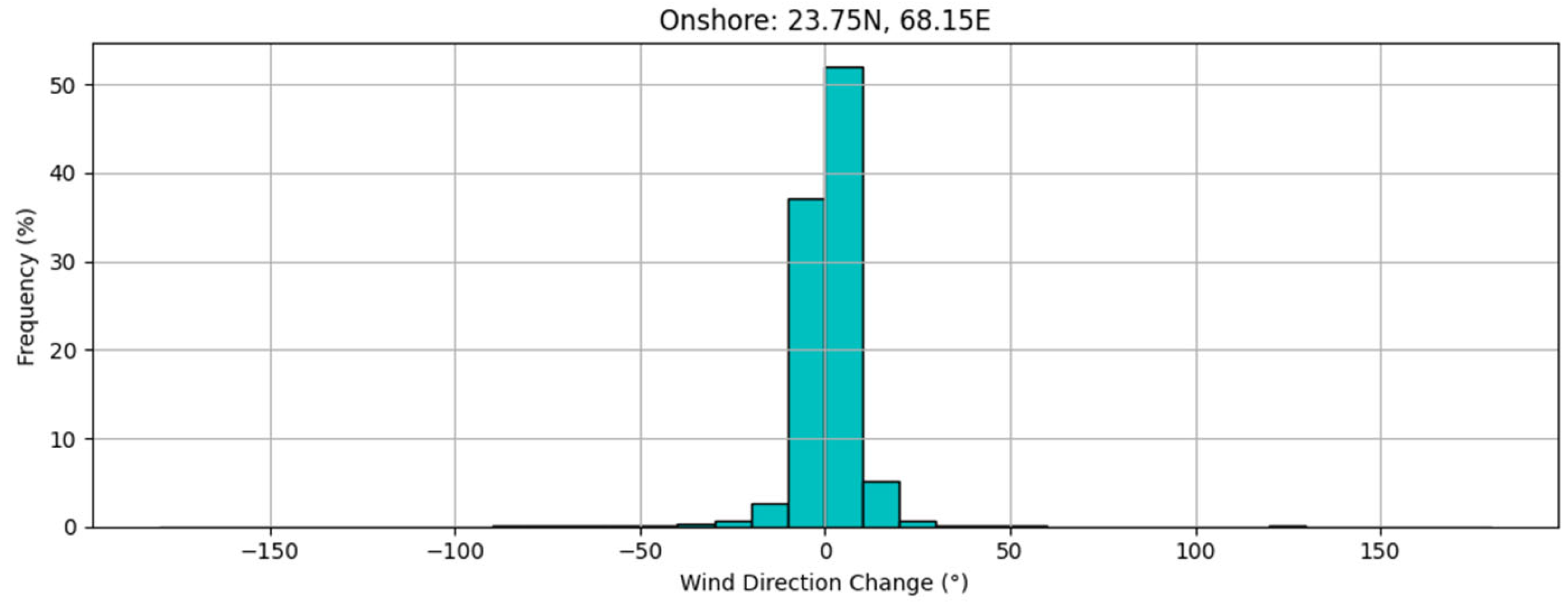
A further analysis of variations between consecutive measurements shows low directional variability at both sites (Figure 13 and Figure 14), with more than 80% of changes in wind direction being less than 10°. Such stability in direction facilitates turbine control and adjustment, thereby minimising losses due to continuous adjustments.

The two selected locations demonstrate wind conditions that are comparable to the distribution of wind speed exhibited by Türkiye’s turbine dataset used for the training of ML and DL models. In particular, both show a predominance of moderate speeds (between 3 and 12 m/s). While the prevailing wind directions are not identical, the similarity in wind speed distribution supports the applicability of the models to these sites [57]. The variation in prevailing wind regimes represents a potential limitation of the study, but the adopted strategy of using direction variability rather than absolute direction helps to mitigate its impact.

4.4. Producibility of the Proposed Wind Farm

Following the selection of both onshore and offshore sites, a simulation of annual energy producibility was carried out. Initially, estimations for both sites were based solely on the turbine’s Theoretical Power Curve. However, this approach does not account for wake losses between turbines nor for grid losses.

To obtain more realistic estimates, the two datasets were then processed by the optimised RF model. Unlike the theoretical curve, the RF model was trained on a real dataset and therefore accounts for various real conditions that can lead to losses, such as wake effect losses. Nevertheless, it does not include grid losses.

To address this, the gross production results obtained from both the theoretical and RF models were adjusted for grid losses, which accounted for 1.91% for offshore and 1.7% for onshore. These values were based on a cable length of 30 km and 5 km, respectively. Furthermore, wake losses were considered by applying wake loss factor of 90% to the production obtained from the theoretical power curve.

As shown in

Table 4. Annual energy producibility in GWh/year of a 5 × 5 wind farm simulated at the selected offshore and onshore sites in Pakistan. Values are estimated using both the trained Random Forest (RF) model and the Theoretical Power Curve. “Gross production” refers to output without accounting for energy losses. “Net production” incorporates grid losses (for RF model) and both grid and wake losses (for theoretical model).

	Producibility [GWh/y]
Site	Trained RF Model: Gross Production	Theoretical Power Curve: Gross Production	Trained RF Model: Net Production	Theoretical Power Curve: Net Production
Offshore	221.3	302.6	217.1	267.1
Onshore	244.9	333.3	240.8	294.9

and

Table 5. Capacity Factor (%) of the 5 × 5 wind farm at the offshore and onshore sites in Pakistan. The values are derived from the trained Random Forest (RF) model and the Theoretical Power Curve, both in gross and net terms. Net values account for grid losses in the RF model and both wake and grid energy losses in the theoretical model. The results show that the theoretical approach consistently overestimates performance.

	Capacity Factor [%]
Site	Trained RF Model: Gross Production	Theoretical Power Curve: Gross Production	Trained RF Model: Net Production	Theoretical Power Curve: Net Production
Offshore	28.1%	38.4%	27.5%	33.9%
Onshore	31.1%	42.3%	30.5%	37.4%

, the theoretical power curve consistently overestimated both annual energy production and capacity factors for both sites. When adjusted for wake and grid losses, the net production values are substantially reduced, leading to more closely aligned values with the RF model outputs.

The RF model conversely provides more conservative yet realistic estimates. For example, the offshore site shows a reduction in capacity factor from 33.9% (theoretical) to 27.5% (RF model), while the onshore site drops from 37.4% to 30.5%. These differences underscore the significant impact of wake losses, which can reduce predicted energy output by up to 20%.

In all estimation methods, the onshore site consistently exhibited higher producibility and CF than the offshore site. This suggests more favourable wind conditions or operating conditions at the onshore location.

These results highlight the necessity of incorporating wake effects and real-world operating conditions into producibility assessments, thereby preventing the overestimation of wind farm performance.

4.5. Economic Analysis Results

The economic analysis indicated that, given the offshore site’s distance from the coast (30 km) and seabed depth (28 m), the most cost-effective solution for the project was the use of a jacket foundation and a grid connection in HVAC. The results presented in

Table 6. CAPEX and OPEX of the offshore wind farm (values in USD₂₀₂₄m).

Foundation (Jacket)	Grid (HVAC)	Installation	Turbines	Total CAPEX
65.612	36.679	102.157	151.395	355.843
				Annual OPEX
				7.117

were obtained for the various CAPEX and OPEX for the offshore facility.

Based on these costs, the LCOE for the offshore site was calculated by considering two different estimates of producibility:

• LCOE = 0.120 USD/kWh using the net producibility calculated through the ML model.
• LCOE = 0.097 USD/kWh using the net producibility estimated through the Theoretical Power Curve.

The findings demonstrated that utilising a more realistic model (based on real data and operating losses) results in a higher LCOE, reflecting more conservative energy production close to real operating conditions. Conversely, utilising the theoretical curve results in an underestimation of the LCOE, owing to its overestimation of producibility.

As for the onshore plant, the CAPEX and annual OPEX values are shown in

Table 7. CAPEX and OPEX of the onshore wind farm (values in USD₂₀₂₄m).

Foundation	Turbines	Other CAPEX	Total CAPEX
8.598	132.580	23.924	165.101
			Annual OPEX
			2.476

.

The LCOE was also calculated for the onshore plant based on the producibility estimated with the two approaches:

• LCOE = 0.059 USD/kWh using net producibility calculated through the ML model.
• LCOE = 0.048 USD/kWh using the net producibility estimated through the Theoretical Power Curve.

As was the case in the offshore context, it was found that utilising the theoretical curve resulted in an underestimation of LCOE, due to an overestimation of producibility. In contrast, the ML model, based on real data, returns a more realistic and conservative value.

In the IRENA 2024 report (“Renewable Power Generation Costs in 2023”) [64], the average LCOE for onshore wind power plants in Pakistan is approximately 0.06 USD/kWh. This value is perfectly aligned with the figure obtained in the present study using the ML model (0.059 USD/kWh), confirming the reliability and consistency of the model used with market values. Furthermore, data published by NEPRA [13] indicates that the actual payment recognised for onshore wind power in Pakistan is approximately 0.046 USD/kWh, which is marginally lower than the theoretical LCOE calculated in the study (0.048 USD/kWh).

This suggests that it is not merely beneficial but rather essential to implement support measures and investment incentives particularly for offshore wind projects in order to attract private investment in Pakistan. Such measures could help bridge the gap between the modelled LCOE values and the levels observed in more mature markets, thus improving the feasibility of wind power deployment in the Pakistani national context.

5. Conclusions

The accurate estimation of the energy producibility of a wind farm constitutes a pivotal challenge, particularly in the context of phenomena such as aerodynamic losses and wake effects. This study has demonstrated that the exclusive utilisation of the theoretical power curve can result in substantial overestimations, thereby validating the employment of more sophisticated ML and DL models trained upon real operational data.

It was evident from the initial operational dataset that there was a discrepancy between the recorded power output and the power calculated via the theoretical power curve. Indeed, it was determined that the nominal power output is achieved at higher wind speeds. An R² between theoretical and actual of approximately 0.88 was observed, which later served as a baseline.

Following the training of the ML and DL models, the R² baseline was surpassed by all five models. However, the Random Forest was identified as the most effective ML algorithm in this instance, attaining a test R² of over 90% and a total R² of 97%.

Following a transductive transfer learning approach, the application of the chosen ML model to the two selected sites, one onshore and one offshore, revealed that using ML models results in more conservative estimates than those derived from a theoretical power curve. Indeed, neglecting grid losses, and most significantly, wake losses, can lead to an overestimation of producibility by up to 20%.

The economic analysis showed that the ML model yielded a higher LCOE than the theoretical power curve, thus reflecting a more realistic assessment of operating losses. At the offshore site, the LCOE calculated with the ML model was 0.120 USD/kWh, compared with 0.097 USD/kWh for the theoretical curve. The ML model produced more realistic production costs, which are higher and thus require supportive policies and incentives to make offshore projects sustainable.

For the onshore site, the LCOE of 0.059 USD/kWh estimated by the ML model is in line with the average value reported by IRENA for Pakistan (~0.06 USD/kWh) and only slightly higher than the price recognised by NEPRA (0.046 USD/kWh). This confirms the reliability of the estimates and indicates that, at present, onshore wind is a safer and more affordable option for investors than offshore.

However, since the application of ML and DL techniques may introduce a potential risk of overfitting—which may reduce predictive reliability on unseen data—further research should focus on expanding datasets to utilise a wider range of environmental and operational conditions, as well as developing more advanced modelling approaches. Moreover, a considerable limitation of this study is the reliance on an onshore SCADA dataset for model training for both the onshore and the offshore scenarios. While the dataset under consideration effectively captures wake losses and provides reliable operational information, it does not include offshore-specific variables such as turbulence intensity, gusts, or sea wave characteristics, which may significantly affect offshore wind farm performance. Future studies should therefore incorporate offshore datasets and additional environmental parameters in order to address this issue.

These efforts are essential to improve the accuracy and robustness of producibility assessments, ultimately supporting more effective planning and deployment of wind energy projects in Pakistan.

References

1. Filonchyk, M.; Peterson, M.P.; Zhang, L.; Hurynovich, V.; He, Y. Greenhouse Gases Emissions and Global Climate Change: Examining the Influence of CO2, CH4, and N2O. Sci. Total Environ. 2024, 935, 173359. [Google Scholar] [CrossRef]
2. IEA. Global Energy Review 2025; IEA: Paris, France, 2025. [Google Scholar]
3. World Energy Transitions Outlook 2024. Available online: https://www.irena.org/Publications/2024/Nov/World-Energy-Transitions-Outlook-2024 (accessed on 27 June 2025).
4. Climate Action Support 2024. Available online: https://www.irena.org/Publications/2024/Nov/Climate-Action-Support-2024 (accessed on 27 June 2025).
5. Kim, J.; Jaumotte, F.; Panton, A.J.; Schwerhoff, G. Energy Security and the Green Transition. Energy Policy 2025, 198, 114409. [Google Scholar] [CrossRef]
6. IRENA. Renewable Capacity Statistics 2025; International Renewable Energy Agency: Abu Dhabi, United Arab Emirates, 2025. [Google Scholar]
7. IRENA. Renewable Power Generation Costs in 2024; International Renewable Energy Agency: Abu Dhabi, United Arab Emirates, 2025. [Google Scholar]
8. Yu, H.; Wen, B.; Zahidi, I.; Chow, M.F.; Liang, D.; Madsen, D.Ø. The Critical Role of Energy Transition in Addressing Climate Change at COP28. Results Eng. 2024, 22, 102324. [Google Scholar] [CrossRef]
9. Qudrat-Ullah, H. A Review and Analysis of Renewable Energy Policies and CO2 Emissions of Pakistan. Energy 2022, 238, 121849. [Google Scholar] [CrossRef]
10. Ahmad, R.; Liu, G.; Rehman, S.A.U.; Fazal, R.; Gao, Y.; Xu, D.; Agostinho, F.; Almeida, C.M.V.B.; Giannetti, B.F. Pakistan Road towards Paris Agreement: Potential Decarbonization Pathways and Future Emissions Reduction by a Developing Country. Energy 2025, 314, 134075. [Google Scholar] [CrossRef]
11. Adil, L.; Eckstein, D.; Künzel, V. Laura Schäfer Climate Risk Index 2025|Germanwatch e.V. Available online: https://www.germanwatch.org/en/cri (accessed on 30 June 2025).
12. Sustainable Development Policy Institute. Annual State of Renewable Energy Report Pakistan 2024; SDPI: Islamabad, Pakistan, 2024. [Google Scholar]
13. National Electric Power Regulatory Authority. State of the Industry Report 2024; NEPRA: Islamabad, Pakistan, 2024. [Google Scholar]
14. Saulat, H.; Khan, M.M.; Aslam, M.; Chawla, M.; Rafiq, S.; Zafar, F.; Khan, M.M.; Bokhari, A.; Jamil, F.; Bhutto, A.W.; et al. Wind Speed Pattern Data and Wind Energy Potential in Pakistan: Current Status, Challenging Platforms and Innovative Prospects. Environ. Sci. Pollut. Res. 2021, 28, 34051–34073. [Google Scholar] [CrossRef]
15. Ali, B.; Abbas, G.; Memon, A.; Mirsaeidi, S.; Koondhar, M.A.; Chandio, S.; Channa, I.A. A Comparative Study to Analyze Wind Potential of Different Wind Corridors. Energy Rep. 2023, 9, 1157–1170. [Google Scholar] [CrossRef]
16. Tahir, Z.u.R.; Abdullah, M.; Ahmad, S.; Kanwal, A.; Farhan, M.; Saeed, U.B.; Ali, T.; Amin, I. An Approach to Assess Offshore Wind Power Potential Using Bathymetry and Near-Hub-Height Reanalysis Data. Ocean. Eng. 2023, 280, 114458. [Google Scholar] [CrossRef]
17. Desalegn, B.; Gebeyehu, D.; Tamrat, B.; Tadiwose, T.; Lata, A. Onshore versus Offshore Wind Power Trends and Recent Study Practices in Modeling of Wind Turbines’ Life-Cycle Impact Assessments. Clean. Eng. Technol. 2023, 17, 100691. [Google Scholar] [CrossRef]
18. Xin, Y.; Bin Dost, M.K.; Akram, H.; Watto, W.A. Analyzing Pakistan’s Renewable Energy Potential: A Review of the Country’s Energy Policy, Its Challenges, and Recommendations. Sustainability 2022, 14, 16123. [Google Scholar] [CrossRef]
19. National Transmission and Despatch Company. Indicative Generation Capacity Expansion Plan (IGCEP 2024-34); NTDC: Islamabad, Pakistan, 2024. [Google Scholar]
20. Ministry of Energy (Power Division). National Electricity Plan 2023–2027; A Block, Pak Secretariat: Islamabad, Pakistan, 2023. [Google Scholar]
21. NEPRA|CTBCM. Available online: https://www.nepra.org.pk/ctbcm.php (accessed on 30 June 2025).
22. Wang, Y.; Duan, X.; Song, D.; Zou, R.; Zhang, F.; Li, Y. Wind Power Curve Modeling with Large-Scale Generalized Kernel-Based Regression Model. IEEE Trans. Sustain. Energy 2023, 14, 2121–2132. [Google Scholar] [CrossRef]
23. Sun, Y.; Li, Y.; Wang, R.; Ma, R. Modelling Potential Land Suitability of Large-Scale Wind Energy Development Using Explainable Machine Learning Techniques: Applications for China, USA and EU. Energy Convers. Manag. 2024, 302, 118131. [Google Scholar] [CrossRef]
24. Karaman, Ö.A. Prediction of Wind Power with Machine Learning Models. Appl. Sci. 2023, 13, 11455. [Google Scholar] [CrossRef]
25. Hulio, Z.H. Assessment of Wind Characteristics and Wind Power Potential of Gharo, Pakistan. J. Renew. Energy 2021, 2021, 8960190. [Google Scholar] [CrossRef]
26. Burney, S.M.A.; Drakhshan, K.; Karim, S. Forecasting Wind Speed Using Machine Learning ANN Models at 4 Distinct Heights at Different Potential Locations in Pakistan. WSEAS Trans. Comput. 2023, 22, 127–141. [Google Scholar] [CrossRef]
27. Tahir, Z.U.R.; Kanwal, A.; Afzal, S.; Ali, S.; Hayat, N.; Abdullah, M.; Saeed, U.B. Wind Energy Potential and Economic Assessment of Southeast of Pakistan. Int. J. Green. Energy 2021, 18, 1–16. [Google Scholar] [CrossRef]
28. Dataset. Available online: https://www.kaggle.com/datasets/berkerisen/wind-turbine-scada-dataset (accessed on 28 May 2025).
29. Shen, W.; Chen, X.; Qiu, J.; Hayward, J.A.; Sayeef, S.; Osman, P.; Meng, K.; Dong, Z.Y. A Comprehensive Review of Variable Renewable Energy Levelized Cost of Electricity. Renew. Sustain. Energy Rev. 2020, 133, 110301. [Google Scholar] [CrossRef]
30. Ozbak, M.; Ghazizadeh-Ahsaee, M.; Ahrari, M.; Jahantigh, M.; Mirshekar, S.; Mirmozaffari, M.; Aranizadeh, A. Improving Power Output Wind Turbine in Micro-Grids Assisted Virtual Wind Speed Prediction. Sustain. Oper. Comput. 2024, 5, 119–130. [Google Scholar] [CrossRef]
31. IEC 61400-12-1; Wind Energy Generation Systems—Part 12-1: Power Performance Measurements of Electricity Producing Wind Turbines. International Electrotechnical Commission: Geneva, Switzerland, 2022.
32. Sireesha, P.V.; Thotakura, S. Wind Power Prediction Using Optimized MLP-NN Machine Learning Forecasting Model. Electr. Eng. 2024, 106, 7643–7666. [Google Scholar] [CrossRef]
33. Liu, Y.; Guan, L.; Hou, C.; Han, H.; Liu, Z.; Sun, Y.; Zheng, M. Wind Power Short-Term Prediction Based on LSTM and Discrete Wavelet Transform. Appl. Sci. 2019, 9, 1108. [Google Scholar] [CrossRef]
34. Mustaffa, Z.; Sulaiman, M.H. Random Forest Based Wind Power Prediction Method for Sustainable Energy System. Clean. Energy Syst. 2025, 12, 100210. [Google Scholar] [CrossRef]
35. Trizoglou, P.; Liu, X.; Lin, Z. Fault Detection by an Ensemble Framework of Extreme Gradient Boosting (XGBoost) in the Operation of Offshore Wind Turbines. Renew. Energy 2021, 179, 945–962. [Google Scholar] [CrossRef]
36. Park, S.; Jung, S.; Lee, J.; Hur, J. A Short-Term Forecasting of Wind Power Outputs Based on Gradient Boosting Regression Tree Algorithms. Energies 2023, 16, 1132. [Google Scholar] [CrossRef]
37. Singh, U.; Rizwan, M.; Alaraj, M.; Alsaidan, I. A Machine Learning-Based Gradient Boosting Regression Approach for Wind Power Production Forecasting: A Step towards Smart Grid Environments. Energies 2021, 14, 5196. [Google Scholar] [CrossRef]
38. Waluyo, N.R.; Astuti, W.; Ihsan, A.F. Anomaly Detection in Gas Pipes with an Ensemble Learning Approach: Combination of Random Forest and GBoost. In Proceedings of the 2024 International Conference on Intelligent Cybernetics Technology and Applications, ICICyTA 2024, Bali, Indonesia, 17–19 December 2024; pp. 55–59. [Google Scholar] [CrossRef]
39. Testasecca, T.; Maniscalco, M.P.; Brunaccini, G.; Airò Farulla, G.; Ciulla, G.; Beccali, M.; Ferraro, M. Toward a Digital Twin of a Solid Oxide Fuel Cell Microcogenerator: Data-Driven Modelling. Energies 2024, 17, 4140. [Google Scholar] [CrossRef]
40. Sarker, I.H. Machine Learning: Algorithms, Real-World Applications and Research Directions. SN Comput. Sci. 2021, 2, 160. [Google Scholar] [CrossRef]
41. Liu, Z.; Guo, H.; Zhang, Y.; Zuo, Z. A Comprehensive Review of Wind Power Prediction Based on Machine Learning: Models, Applications, and Challenges. Energies 2025, 18, 350. [Google Scholar] [CrossRef]
42. Glossary—U.S. Energy Information Administration (EIA). Available online: https://www.eia.gov/tools/glossary/index.php?id=Capacity_factor (accessed on 30 June 2025).
43. Feng, Y.; Gong, D.; Jiang, S.; Zhao, L.; Cui, N. National-Scale Development and Calibration of Empirical Models for Predicting Daily Global Solar Radiation in China. Energy Convers. Manag. 2020, 203, 112236. [Google Scholar] [CrossRef]
44. Das, K.; Kumar, R.; Krishna, A. Analyzing Electric Vehicle Battery Health Performance Using Supervised Machine Learning. Renew. Sustain. Energy Rev. 2024, 189, 113967. [Google Scholar] [CrossRef]
45. Dasi, H.; Ying, Z.; Ashab, M.F. Bin Proposing Hybrid Prediction Approaches with the Integration of Machine Learning Models and Metaheuristic Algorithms to Forecast the Cooling and Heating Load of Buildings. Energy 2024, 291, 130297. [Google Scholar] [CrossRef]
46. Satymov, R.; Bogdanov, D.; Breyer, C. Techno-Economics of Offshore Wind Power in Global Resolution. Appl. Energy 2025, 393, 125980. [Google Scholar] [CrossRef]
47. Bosch, J.; Staffell, I.; Hawkes, A.D. Temporally Explicit and Spatially Resolved Global Offshore Wind Energy Potentials. Energy 2018, 163, 766–781. [Google Scholar] [CrossRef]
48. Cavazzi, S.; Dutton, A.G. An Offshore Wind Energy Geographic Information System (OWE-GIS) for Assessment of the UK’s Offshore Wind Energy Potential. Renew. Energy 2016, 87, 212–228. [Google Scholar] [CrossRef]
49. Sens, L.; Neuling, U.; Kaltschmitt, M. Capital Expenditure and Levelized Cost of Electricity of Photovoltaic Plants and Wind Turbines—Development by 2050. Renew. Energy 2022, 185, 525–537. [Google Scholar] [CrossRef]
50. Bosch, J.; Staffell, I.; Hawkes, A.D. Global Levelised Cost of Electricity from Offshore Wind. Energy 2019, 189, 116357. [Google Scholar] [CrossRef]
51. Euro Foreign Exchange Reference Rates. Available online: https://www.ecb.europa.eu/stats/policy_and_exchange_rates/euro_reference_exchange_rates/html/index.en.html (accessed on 1 July 2025).
52. Consumer Price Index, 1913-|Federal Reserve Bank of Minneapolis. Available online: https://www.minneapolisfed.org/about-us/monetary-policy/inflation-calculator/consumer-price-index-1913- (accessed on 1 July 2025).
53. Dato, P.; Dioha, M.; Hessou, H.; Houenou, B.; Mukhaya, B.; Okyere, M.A.; Odarno, L. Computation of Weighted Average Cost of Capital (WACC) in the Power Sector for African Countries and the Implications for Country-Specific Electricity Technology Cost. Appl. Energy 2025, 397, 126333. [Google Scholar] [CrossRef]
54. Wind Turbine Scada Dataset. Available online: https://www.kaggle.com/datasets/berkerisen/wind-turbine-scada-dataset/data (accessed on 27 June 2025).
55. Position of the Wind Turbine—40°35’07.6″ N 28°59′25.3″ E—Google Maps. Available online: https://www.google.com/maps/place/40%C2%B035’07.6%22N+28%C2%B059’25.3%22E/@40.5851806,28.9897199,833m/data=!3m1!1e3!4m4!3m3!8m2!3d40.5854444!4d28.9903611!5m1!1e4?hl=en-US&entry=ttu&g_ep=EgoyMDI1MDYyMy4yIKXMDSoASAFQAw%3D%3D (accessed on 27 June 2025).
56. N117/3600—Nordex, SE. Available online: https://www.nordex-online.com/en/product/n117-3600/ (accessed on 27 June 2025).
57. Chatterjee, J.; Dethlefs, N. Deep Learning with Knowledge Transfer for Explainable Anomaly Prediction in Wind Turbines. Wind. Energy 2020, 23, 1693–1710. [Google Scholar] [CrossRef]
58. Zahid, M.; Rasul, G. Thermal Classification of Pakistan. Atmos. Clim. Sci. 2011, 01, 206–213. [Google Scholar] [CrossRef]
59. Adeel, M.; Razzak, A.; Riaz, S.M.F.; Iqbal, M.J. Impact of Sea Surface Temperature in the Arabian Sea on the Variability of Summer Monsoon Rainfall over Pakistan Region. Dyn. Atmos. Ocean. 2024, 107, 101482. [Google Scholar] [CrossRef]
60. Copernicus Climate Change Service, Climate Data Store. ERA5 Hourly Data on Single Levels from 1940 to Present; Copernicus Climate Change Service (C3S) Climate Data Store (CDS): 2023. Available online: https://cds.climate.copernicus.eu/datasets/reanalysis-era5-single-levels?tab=overview (accessed on 28 May 2025).
61. Sharma, P.K.; Warudkar, V.; Ahmed, S. Effect of Atmospheric Stability on the Wind Resource Extrapolating Models for Large Capacity Wind Turbines: A Comparative Analysis of Power Law, Log Law and Deaves and Harris Model. Energy Procedia 2019, 158, 1235–1240. [Google Scholar] [CrossRef]
62. Golbazi, M.; Archer, C.L. Methods to Estimate Surface Roughness Length for Offshore Wind Energy. Adv. Meteorol. 2019, 2019, 5695481. [Google Scholar] [CrossRef]
63. Levin, N.; Ben-Dor, E.; Kidron, G.J.; Yaakov, Y. Estimation of Surface Roughness (Z0) Cover a Stabilizing Coastal Dune Field Based on Vegetation and Topography. Earth Surf. Process Landf. 2008, 33, 1520–1541. [Google Scholar] [CrossRef]
64. IRENA. Renewable Power Generation Costs in 2023; International Renewable Energy Agency: Abu Dhabi, United Arab Emirates, 2024. [Google Scholar]
Figure 2. Different approaches to the training phase of ML models: (a) Sequential Training, and (b) Parallel Training.
Energies 18 05080 g002
Figure 3. Different DL architectures: (a) Recurrent Neural Network, and (b) Feed-Forward Neural Network.
Energies 18 05080 g003
Figure 4. Grid losses (HVAC and HVDC) as functions of distance to the substation.
Energies 18 05080 g004
Figure 5. Geographical location of the analysed wind turbine.
Energies 18 05080 g005
Figure 6. Wind rose extracted from the dataset for the turbine location in Türkiye.
Energies 18 05080 g006
Figure 7. Distribution of wind direction changes (in degrees) expressed as percentages over the entire year of data acquisition.
Energies 18 05080 g007
Figure 8. Exclusive Economic Zone (EEZ) of Pakistan.
Energies 18 05080 g008
Figure 9. Comparison between the theoretical power curve and the median real power from the Turkish dataset. The blue band represents the 5th–95th percentile range.
Energies 18 05080 g009
Figure 10. Model bathymetry for the EEZ in Pakistan, with the two chosen sites highlighted.
Energies 18 05080 g010
Figure 11. Wind rose for the offshore site.
Energies 18 05080 g011
Figure 12. Wind rose for the onshore site.
Energies 18 05080 g012
Figure 13. Distribution of wind direction changes (in degrees) expressed as percentages over the entire year of data for the offshore site.
Energies 18 05080 g013
Figure 14. Distribution of wind direction changes (in degrees) expressed as percentages over the entire year of data for the onshore site.
Energies 18 05080 g014