Abstract
The On-Load Tap Changer (OLTC), as a critical component of transformers, undergoes frequent switching operations that can lead to faults such as contact wear and arc discharge, which are often difficult to detect at an early stage using traditional monitoring methods. In particular, dissolved gas analysis (DGA) in OLTC oil is challenged by the unique oil gas decomposition mechanisms and the presence of background noise, making conventional DGA criteria less effective. Moreover, OLTC oil monitoring data are typically obtained through intermittent sampling, resulting in sparse time series with low resolution that complicate fault prediction. To address these challenges, this paper proposes an integrated framework combining LGOD-based anomaly detection, Locally Weighted Regression (LWR) for data repair, and the ETSformer temporal prediction model. This approach effectively identifies and corrects anomalies, restores the dynamic variation trends of gas concentrations, and enhances prediction accuracy through deep temporal modeling, thereby providing more reliable data support for OLTC state assessment and fault diagnosis. Experimental results demonstrate that the proposed method significantly improves prediction accuracy, enhances sensitivity to gas concentration evolution, and exhibits robust adaptability under both normal and fault scenarios. Furthermore, ablation experiments confirm that the observed performance gains are attributable to the complementary contributions of LGOD, LWR, and ETSformer, rather than any single component alone, highlighting the effectiveness of the integrated approach.
1. Introduction
The On-Load Tap Changer (OLTC), as a critical component of transformers, directly influences the voltage regulation capability of power systems and the operational safety of equipment [1]. Due to the frequent switching operations performed during OLTC operation, its internal contacts, transition resistance, and insulation media are subjected to combined effects of arc discharge, thermal stress, and electrical stress over prolonged periods, which easily lead to contact wear, carbon accumulation, abnormal discharges, and other faults [2]. Early manifestations of OLTC faults are typically latent and difficult to detect through conventional operational parameters. However, once faults accumulate to a critical threshold, severe consequences such as contact welding, open or short circuit of the transition resistance may occur, thereby jeopardizing the safety and stability of transformer operation and the entire power system [3].
Dissolved Gas Analysis (DGA) is a well-established technique for transformer fault diagnosis, providing valuable insights into the types and concentrations of gases dissolved in insulating oil [4,5]. In on-load tap changers (OLTCs), however, frequent switching operations introduce unique phenomena such as arcing and contact wear, which alter oil decomposition pathways and result in gas compositions distinct from those in the transformer main tank. Among these, acetylene (C2H2) is particularly complex: while commonly recognized as an indicator of severe internal faults such as arcing, it is also a natural byproduct of normal OLTC operation, thereby complicating fault identification [6,7,8].
Although DGA is critical for OLTC fault diagnosis, gas monitoring in OLTC oil is still predominantly performed through intermittent sampling, constrained by two fundamental factors. First, existing commercial gas monitors face inherent limitations in OLTC applications. Most devices require manual on-site sampling at intervals of weeks, and even online monitors often struggle to achieve stable daily or higher-frequency measurements due to restricted installation space, severe mechanical vibrations, and electromagnetic interference during switching operations. Moreover, high-frequency monitoring may cause sensor drift and oil contamination, further reducing data reliability. Second, OLTCs typically operate at relatively high switching frequencies. The OLTC undergoes multiple switching operations per day, each of which induces short-lived peaks in gas concentrations lasting only one to two hours. Conventional low-frequency sampling, conducted every few days, is unable to capture these transient variations, leading to highly discrete gas profiles and substantially limiting the accuracy of trend analysis and fault prediction. Though recent research has sought to refine DGA techniques to alleviate the effects of sparse spatiotemporal data [9,10], systematic investigations dedicated to OLTC applications remain limited. Established interpretation methods—such as the key gas ratio approach and the Duval triangle method—are widely applied in main transformer tank diagnostics [11], yet have not been adequately extended to OLTCs. Addressing this gap is essential to advance reliable fault diagnosis in tap changers.
At present, predictive approaches for dissolved gas analysis (DGA) primarily encompass statistical forecasting [12], machine learning [13], and deep learning methods [14]. Statistical models, such as grey models and traditional time series approaches, are capable of capturing overall data trends but often suffer from limited accuracy when confronted with non-stationary and nonlinear sequences [15]. To improve predictive performance, machine learning methods, particularly gradient boosting decision trees (GBDT) and their advanced variants, have been widely adopted for dissolved gas concentration forecasting [16,17]. While these models are effective in utilizing structured features, they are typically constructed on static representations and thus fail to adequately capture the temporal evolution of gas concentrations, which is critical given the intermittent and dynamic nature of OLTC oil monitoring. More recently, deep learning techniques have emerged as powerful alternatives, demonstrating superior performance in modeling nonlinear dependencies and temporal dynamics, thereby establishing themselves as the leading direction in DGA-based predictive research [18,19]. In particular, deep neural network-based ensemble frameworks outperform traditional approaches such as logistic regression, random forests, and adaptive boosting by offering stronger nonlinear feature extraction capabilities. Nevertheless, most existing studies focus on specific operating conditions without fully considering the temporal dependencies and spatial correlations inherent in gas evolution, thereby limiting model generalizability. To address these limitations, Transformer architectures have garnered increasing attention due to their advantages in time series modeling [20,21]. LogTrans [22], for instance, improves long-term dependency modeling through local causal convolutions while retaining the global attention mechanism of Transformers to enhance feature extraction from gas concentration variations. Building upon this, Informer [23] introduces a probabilistic sparse self-attention mechanism and a scalable time decomposition strategy, greatly increasing efficiency in long-sequence forecasting. Against this backdrop, ETSformer has recently emerged as a novel time series forecasting model that integrates exponential smoothing attention with frequency-based attention mechanisms, offering enhanced capability in capturing both trend evolution and periodic patterns [24,25,26]. While ETSformer has demonstrated strong performance in generic time series forecasting tasks, it has not yet been applied to dissolved gas analysis. Considering the distinctive characteristics of OLTC oil, where frequent switching operations lead to intermittent gas fluctuations and blurred boundaries between normal and fault-related gas generation, ETSformer provides a promising framework to uncover latent temporal structures and improve the reliability of gas concentration prediction in this domain.
Accurate identification and correction of anomalous data that deviate from normal operating patterns are essential for reliably reflecting the actual operational state and evolutionary trends of the OLTC, thereby enhancing data credibility and improving the effectiveness of fault diagnosis and condition assessment [27,28,29]. In fields such as power equipment monitoring and load sensing, anomaly detection has become a central research focus. Existing methods, such as Local Outlier Factor (LOF) and Isolation Forest (IF) [30,31], have been successfully applied to various anomaly detection scenarios. However, these approaches predominantly rely on global criteria for anomaly identification, exhibiting limited sensitivity to local anomalies and often failing to detect subtle deviations [32]. To address this limitation, this study introduces a novel anomaly detection method based on the Local Gradient of Outlier Degree (LGOD), designed to improve the recognition of localized anomalies.
In addition, Local Weighted Regression (LWR) is employed to further correct the identified anomalous data, thereby improving data quality and ensuring temporal continuity [33]. LWR is widely recognized for its ability to handle nonlinear and non-stationary data, providing flexible local fitting that preserves underlying patterns without imposing rigid global assumptions. It has been successfully applied in domains such as environmental monitoring and sensor calibration, where irregular data frequently occur [34,35]. However, its performance is strongly influenced by the choice of kernel bandwidth and weighting schemes, which may result in over-smoothing or underfitting when applied to highly volatile signals. Within the proposed framework, LWR is integrated to exploit its strengths in local approximation while mitigating its limitations through complementary combination with LGOD and ETSformer. This integration enables a more accurate characterization of OLTC condition evolution trends under intermittent monitoring regimes.
Existing studies on OLTC dissolved gas prediction have achieved progress through statistical and deep learning approaches; however, challenges remain due to data sparsity, measurement noise, and vulnerability to outliers, which limit their applicability in real monitoring environments. Motivated by these limitations, this study develops an integrated predictive framework that combines LGOD-based anomaly detection, LWR-based data reconstruction, and the ETSformer deep time series forecasting model. The proposed method effectively improves data quality, enhances temporal continuity, and strengthens the modeling of dynamic gas evolution. Experimental and ablation results demonstrate that the framework significantly outperforms conventional methods, while the complementary contributions of its components provide clear evidence of its necessity and practical value.
2. Algorithm Introduction
2.1. An LGOD-Based Method for Anomaly Detection in Time Series Data
Transient disturbances induced by OLTC operations can lead to localized fluctuations in dissolved gas concentration measurements, resulting in anomalous data patterns [36]. Therefore, it is essential to incorporate an anomaly detection algorithm with fine-grained sensitivity to accurately identify such deviations. To address this need, this study proposes a novel anomaly detection method for dissolved gas data based on the Local Gradient of Outlier Degree (LGOD). This method quantifies variations in the local resultant force experienced by data points across multiple neighborhood scales, thereby enabling effective discrimination of outliers.
The local resultant force characterizes the aggregate influence—conceptualized as gravitational attraction—exerted on a data point by its neighboring points, as illustrated in Figure 1. Based on gravitational theory, the attraction (or force) between two data points Pi and Pj can be defined as follows:
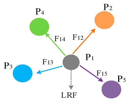
Figure 1.
Local resultant force plot.
Here, G denotes the gravitational constant, mi and mj represent the masses assigned to data points Pi and Pj, respectively, dij denotes the Euclidean distance between the two points, and is the unit vector pointing from Pi to Pj.
By combining the gravitational constant and the masses into a proportionality factor C, the gravitational force expression can be simplified.
As illustrated in Figure 1, the local resultant force is defined as the vector sum of the gravitational influences exerted on data object i by all its neighbors within the k-nearest neighborhood [37]. The corresponding formulation is given by
Here, k denotes the number of nearest neighbors of data point i. The local resultant force (LRF) provides a comprehensive characterization of the spatial distribution and directional influence acting on point i within its neighborhood [38]. The simplified expression for the LRF is given by
Here, wi represents the mass of data object i, which is defined
According to the above definition, points located in low-density regions exhibit stronger local resultant forces due to larger distances and smaller masses, whereas points in high-density regions tend to have weaker local resultant forces as a result of greater mass and mutual gravitational cancellation. Figure 2 illustrates the local resultant force as the number of neighbors k increases. By comparing Figure 2a,b, it is evident that the local resultant force of point P2 changes minimally, while that of point P1 exhibits a pronounced variation. This indicates that different types of points experience significantly distinct changes in their local resultant forces as the neighborhood size expands.
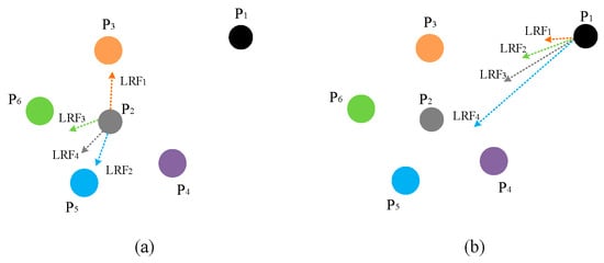
Figure 2.
Distribution of local resultant forces at different types of points. (a) Local resultant force of P2; (b) Local resultant force of P1.
Since the local resultant force directions of outliers or boundary points tend to be aligned, their local resultant force magnitudes increase with the number of neighbors. In contrast, internal points exhibit diverse attraction directions, resulting in negligible local resultant forces as the neighborhood size expands. To quantitatively characterize the LRF, the following metric is defined, as expressed in Equation (6):
Here, denotes the magnitude of the local resultant force acting on data object i with respect to its k neighbors, where K represents the maximum number of neighbors considered for point i. By cumulatively summing the local resultant force magnitudes of data object i across increasing neighborhood sizes, the local resultant force variation rate is obtained. The calculation is formulated as follows:
To enable automatic identification of outliers based on the variation rate, this study employs a hierarchical partitioning method to adaptively determine the threshold. Specifically, the difference in local resultant force variation rates between data objects i and j is defined as LRFVar(i,j), which is computed as follows:
By sorting the local resultant force variation rates of all data objects within the dataset, an LRFList is constructed. The differences in local resultant force variation rates between adjacent data objects in this list are then calculated, where pronounced peaks typically indicate outliers characterized by significantly large variation rates. Accordingly, by setting a threshold τ, values of LRFVar exceeding this threshold are identified as anomalies. The threshold τ is defined as follows:
Here, EX denotes the expected value, and SD represents the standard deviation. The adjustment parameter α within (0,3], with a default value set to 2.5. By applying a positive adjustment to the expected value of the LRFVarList, anomalies can be effectively identified. Based on this principle, the LGOD method ranks the dissolved gas data in OLTC oil according to the variation rate of the local resultant force, enabling automatic anomaly detection without the need for manual intervention or complex assumptions.
2.2. Data Reconstruction Method Based on Locally Weighted Regression
Locally Weighted Regression (LWR) is a non-parametric regression technique widely employed for data reconstruction following anomaly detection. Its core principle lies in assigning weights to data points based on their proximity to the target point, whereby neighboring points receive higher weights while distant points are assigned lower weights. This weighting scheme reduces the influence of remote points on the fitted model, thereby enabling effective capture of local data characteristics [39,40]. The specific procedural steps of LWR are as follows:
First, weights are computed using a Gaussian kernel function [41]. For the data point xt at the current time step t, the weights of its neighboring points are determined based on their distances to xt. The weighting function is specifically defined
Here, wi denotes the weight of the i-th neighboring point, and h is the bandwidth parameter. Within the neighborhood of each data point xt, a weighted linear regression is performed based on the weight distribution. By minimizing the weighted sum of squared residuals, the local regression coefficients are estimated, which are then used to reconstruct the current data point. The regression model is formulated as follows:
Here, β represents the regression coefficients, yi denotes the observed value, and yi′ corresponds to the reconstructed value.
2.3. ETSformer-Based Forecasting Model
The variations in gas concentrations induced by OLTC operations are closely correlated with switching frequency and load fluctuations, necessitating a time series forecasting model capable of simultaneously capturing long-term trends and periodic oscillations [42]. To this end, the ETSformer model is introduced for temporal modeling and prediction of dissolved gas concentrations in oil. ETSformer is an innovative Transformer architecture that integrates an exponential smoothing mechanism [43]. By decomposing the time series into level, growth (trend), and seasonal components layer by layer, it significantly enhances the model’s ability to capture temporal structural biases. Leveraging the expressive power of deep neural networks and an efficient residual learning framework, ETSformer precisely captures the latent trend evolution and periodic fluctuations inherent in the dissolved gas data, effectively modeling their complex dynamic dependencies.
For the problem of dissolved gas prediction in OLTC oil, the data is first modeled as a multivariate time series. Let xt∈Rm denote the feature observation vector at time step t, and yt∈R represent the corresponding gas concentration value. Given the historical feature window Xt−L:t−1 = [xt−L,…,xt−1] and the corresponding gas concentration observations Yt−L:t−1 = [yt−L,…,yt−1], the objective is to predict the gas concentrations for the next H steps, denoted as Yt+1:t+H = [yt+1,…,yt+H]. Here, the look-back window length L defines the number of past observations provided as model input, while the forecasting horizon H specifies the number of future steps to be predicted.
Step 1: Input Embedding.
The modeling process begins with an input embedding module that transforms the raw dissolved gas concentration data within the look-back window into a latent representation space. This is achieved through a temporal convolutional filter [44], which effectively captures short-term correlations among different gas components:
Step 2: Encoder with Growth and Seasonal Decomposition.
Subsequently, the encoder extracts growth and seasonal features of the dissolved gas concentration data through a cascaded, layer-wise mechanism [45]. At each layer, the residual sequence Zt−L:t−1 is taken as input. The Multi-Head Exponential Smoothing Attention (MH-ESA) module and the Frequency Attention (FA) module jointly operate to update the residuals Zt−L:t, while simultaneously generating the latent growth component Bt−L:t and the seasonal component St−L:t. This iterative process allows for progressive refinement and separation of temporal patterns:
Step 3: Level Component Extraction.
In parallel, the level component is dynamically estimated. At each time step t, the level value is computed as a weighted combination of the current level estimate and the extrapolated level-growth prediction from the previous step [45]. This ensures that the level component evolves smoothly while adapting to recent changes:
Step 4: Forecasting Seasonal Dynamics.
For each latent periodic feature dimension within the look-back window, denoted as S(n)t−L:t,i, the Frequency Attention module extrapolates the seasonal component into the forecasting horizon, producing S(n)t:t+H
Finally, the decoder integrates the extracted level, growth, and seasonal components into a coherent prediction framework. By stacking multiple encoder layers and residual connections, ETSformer progressively enhances the representation of dynamic dependencies. The outputs are linearly mapped back from the latent space to the observation space, yielding the multi-step forecasts of dissolved gas concentrations over the future H steps:
As illustrated in Figure 3, the ETSformer-based forecasting framework employs a series of stacked encoders to extract both growth and seasonal features from historical dissolved gas concentration data, while simultaneously utilizing exponential smoothing to update the level component. The final decoder integrates these three structural components—level, growth, and seasonal—to generate accurate and interpretable multi-step predictions of gas concentrations in OLTC oil.
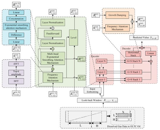
Figure 3.
Architectural framework for predicting gas content in oil based on ETSformer model.
2.4. The Framework of the OLTC Dissolved Gas Prediction Model
The proposed OLTC dissolved gas concentration prediction method, which integrates the LGOD-based outlier detection approach with the ETSformer forecasting model, is illustrated in Figure 4. The overall procedure consists of the following steps:
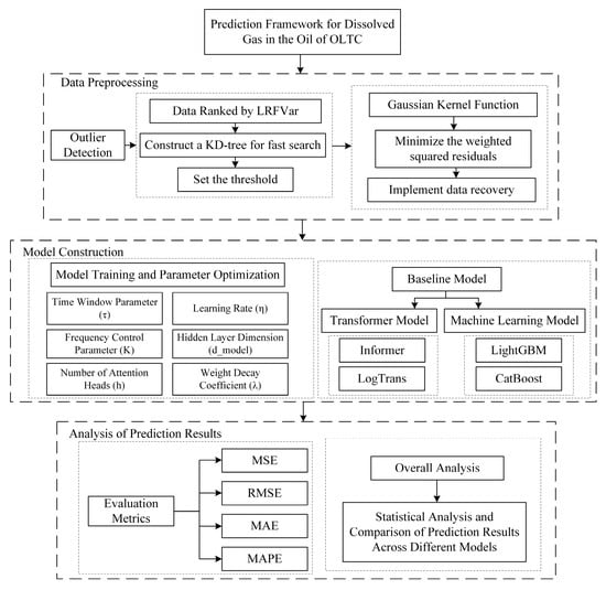
Figure 4.
Flow chart of the proposed prediction method.
Step 1: The original dissolved gas data from the OLTC is first subjected to outlier detection using the LGOD algorithm. Detected outliers are subsequently removed. Local weighted regression is then employed to impute and reconstruct the data, thereby completing the data preprocessing phase.
Step 2: The preprocessed dataset is partitioned into training, validation, and test sets to facilitate subsequent model training and performance evaluation.
Step 3: An ETSformer-based forecasting model is constructed for predicting OLTC dissolved gas concentrations. The training set is fed into the encoder module of the model for learning, during which model parameters are optimized to achieve the best predictive configuration.
Step 4: The trained model is validated using the validation dataset. Furthermore, the predictive performance is compared against various baseline models to rigorously assess the effectiveness of the proposed method in forecasting OLTC dissolved gas concentrations.
In this study, a comprehensive comparative evaluation is conducted to validate the effectiveness of the proposed OLTC dissolved gas concentration forecasting method. The evaluation includes deep learning models such as Transformer, LogTrans, and Informer, as well as machine learning models including LightGBM and CatBoost. To assess the prediction performance of dissolved gas concentrations in OLTC oil, four widely adopted evaluation metrics are employed: Mean Squared Error (MSE), Root Mean Squared Error (RMSE), Mean Absolute Error (MAE), and Mean Absolute Percentage Error (MAPE) [46]. The definitions of these evaluation metrics are presented as follows, where yi denotes the actual measured concentration of a dissolved gas at the i-th time step, and represents the corresponding predicted value generated by the forecasting model.
3. Experimental Results and Analysis
This study initially conducts an in-depth analysis of dissolved gas monitoring data collected from the OLTC oil of a 220 kV power substation in China, spanning from 1 March 2022 to 1 January 2023, comprising a total of 200 gas volume fraction samples. To overcome data limitations, the OLTC oil sampling system was enhanced to achieve stable, near-daily data collection over the course of one year. It should be noted that such high-frequency monitoring remains uncommon in industry due to additional equipment and operational costs, as well as structural constraints in older OLTCs that limit sampling frequency. To address residual data scarcity and sample imbalance, the original dataset is preprocessed using the LGOD anomaly detection algorithm to identify and remove outliers, followed by imputation of missing values to enhance data quality and reliability. Subsequently, the ETSformer model is employed to forecast dissolved gas concentrations in OLTC oil, and its predictive accuracy is rigorously compared against various benchmark models to validate the proposed method’s effectiveness and superiority in practical applications. Furthermore, the study extends to predictive analysis based on an additional set of 50 chromatographic monitoring samples that reflect the entire insulation degradation process of the OLTC. This dataset captures the evolution of dissolved gas concentrations as the OLTC transitions from normal operation to insulation deterioration. By integrating the proposed deep temporal forecasting approach, the analysis effectively uncovers abnormal patterns and dynamic evolution trends inherent in the data.
3.1. Normal Data Preprocessing and Forecasting
The original dissolved gas monitoring data from the OLTC oil of a 220 kV power substation, as shown in Figure 5, includes six key gas species: C2H6, CO, H2, C2H4, CO2, and CH4. Figure 5 provides a direct visualization of the raw OLTC monitoring dataset, illustrating the temporal distribution and baseline characteristics of each gas concentration prior to any preprocessing. It should be noted that C2H2, although a critical diagnostic indicator under fault conditions, is not included in the predictive analysis of this dataset. The overall acetylene concentration measured during normal OLTC operation was consistently close to zero, with only a few scattered points exhibiting abnormal values or abrupt increases. Compared with the more dynamic variations observed in other gases, these limited fluctuations were insufficient to provide meaningful predictive patterns under normal operating conditions. Therefore, C2H2 was excluded from the forecasting experiments at this stage; however, its diagnostic relevance is not overlooked, and it is further analyzed in the subsequent fault evolution study, where acetylene becomes a key indicator of insulation degradation and arc discharge.
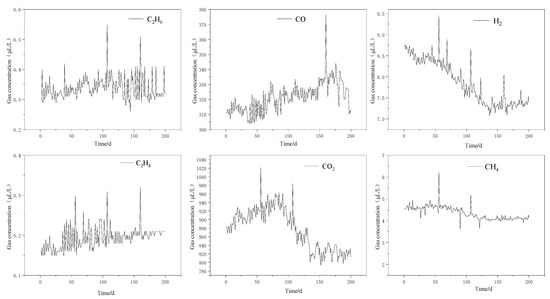
Figure 5.
Raw data diagram of each dissolved gas.
To optimize the model’s training effectiveness and generalization capability, the complete dataset of 200 samples was first partitioned into training and testing subsets at a ratio of 3:1, prior to any preprocessing operations. The proposed preprocessing methodology was then applied exclusively to the training subset: the LGOD anomaly detection algorithm was used to identify and label outliers, followed by the LWR method for data imputation and correction, thereby enhancing data quality and integrity while avoiding information leakage. The reconstructed training set thus retained consistency with expected physical behavior, whereas the testing subset was left unaltered to provide a fair and unbiased evaluation of model generalization. Taking the H2 concentration data from Figure 5 as an illustrative example, Figure 6 shows this procedure in detail: panel (a) presents the raw time series with detected anomalous points highlighted, while panel (b) displays the reconstructed series after anomaly correction, demonstrating improved stability and continuity aligned with physical expectations.
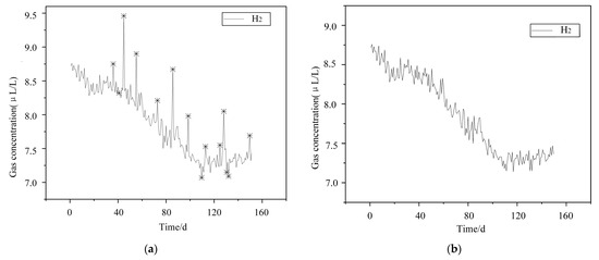
Figure 6.
Graph for Identifying and Repairing Anomalies in H2 Data. (a) Anomaly Detection Plot; (b) Data Repair Plot.The symbol * marks the identified anomaly points.
This study develops a dissolved gas concentration forecasting model for OLTC oil based on the ETSformer architecture, achieving enhanced temporal prediction performance through systematic parameter optimization and structural innovations. The model employs a hierarchical encoder–decoder design, where the encoder consists of two stacked hierarchical layers, each producing a 1024-dimensional latent representation augmented by a 2048-dimensional feedforward neural network for nonlinear feature enhancement. The decoder features a dual-cascade structure that hierarchically extracts multiscale temporal features of gas concentration evolution, combined with an 8-head attention mechanism to effectively capture global dependencies across time steps.
To accommodate the temporal characteristics of dissolved gas concentration, the model input is formulated as a historical look-back window of length L, with the corresponding forecasting horizon denoted as H. Through systematic evaluation and validation by Granger causality tests, the optimal configuration was determined as L = 11 days and H = 7 days. This setting ensures that the historical input window captures sufficient physical diffusion dynamics of gases within the oil, while the prediction horizon provides a practically meaningful forecasting interval for early-warning applications [47].
The optimization strategy adopts a two-stage hyperparameter search framework [48]: in the first stage, grid search identifies the optimal learning rate, with η = 3 × 10⁻⁴ yielding the best convergence on the validation loss; in the second stage, Bayesian optimization determines the frequency control parameter K within {0,1,2,3}, achieving an optimal trade-off between model complexity and generalization at K = 2 [49]. Training is conducted using a progressive learning schedule over 50 iterations, incorporating a dynamic weight decay strategy with linear decay proportional to iteration count. The ETSformer model is constructed and trained on the training dataset, with predictive accuracy rigorously validated against the test set, demonstrating the model’s effectiveness in capturing complex temporal dynamics in dissolved gas concentration forecasting.
The final predictions of gas concentrations based on the trained ETSformer model are illustrated in Figure 7. As shown, the ETSformer’s forecasted curves exhibit a high degree of concordance with the actual observed values, demonstrating superior fitting capability. Notably, the model outperforms comparative baselines, particularly in capturing the fluctuation patterns across multiple gas components, thereby delivering more precise and reliable prediction results.
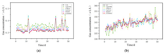
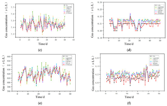
Figure 7.
Prediction curves of each gas content and each model. (a) Prediction plots of various models for C2H6; (b) Prediction plots of various models for CO; (c) Prediction plots of various models for H2; (d) Prediction plots of various models for C2H4; (e) Prediction plots of various models for CO2; (f) Prediction plots of various models for CH4. (The y-axis ranges differ among subplots to better visualize fluctuations of each gas species).
To comprehensively demonstrate the superior performance of the ETSformer model in dissolved gas concentration forecasting, this study conducted detailed predictive analyses and comparative evaluations for six dissolved gases in OLTC oil: CO, C2H4, CO2, C2H6, CH4, and H2. The specific results are summarized in Table 1. The ETSformer model achieved mean absolute percentage errors (MAPE) of 0.81%, 2.57%, 0.73%, 1.57%, 4.57%, and 2.32%, respectively. In comparison, machine learning baseline models LightGBM and CatBoost yielded MAPE values of 7.22%, 7.32%, 6.83%, 4.41%, 14.41%, 9.15% and 6.85%, 6.84%, 5.78%, 4.13%, 12.57%, 8.89%, respectively. Deep learning baselines LogTrans and Informer obtained MAPE values of 4.02%, 4.05%, 4.43%, 3.77%, 9.56%, 6.43% and 4.28%, 4.22%, 3.29%, 2.49%, 7.25%, 5.87%, respectively.

Table 1.
Prediction accuracy of different models for dissolved gas concentrations in OLTC oil (unit: μL/L).
These results clearly indicate that Transformer-based deep learning models outperform traditional machine learning approaches in time series forecasting tasks. Their core advantage lies in the exceptional capability for temporal feature extraction and modeling of global dependencies, effectively preserving the temporal continuity of data and capturing latent patterns. Addressing the challenge posed by discontinuous data acquisition, the ETSformer model integrates an exponential smoothing mechanism that enhances its representation of long-term trend characteristics, enabling robust prediction performance despite extended time intervals caused by intermittent data sampling.
3.2. Ablation Study Comparative Results
To rigorously assess the contribution of each component in the proposed framework, an ablation study was conducted using the training and testing sets. The comparative results for four evaluation metrics, namely MSE, RMSE, MAE, and MAPE, are presented in Figure 8, where Figure 8a–d correspond to MSE, RMSE, MAE, and MAPE, respectively. Specifically, the full model integrating LGOD anomaly detection, LWR data repair, and ETSformer forecasting was compared against three simplified variants: (i) removing LGOD while retaining LWR and ETSformer, (ii) removing LWR while retaining LGOD and ETSformer, and (iii) employing ETSformer alone without preprocessing.
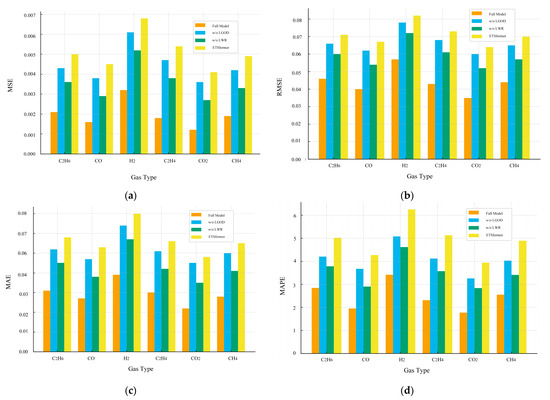
Figure 8.
Ablation study results of different models across four evaluation metrics. (a) Comparison of MSE for each gas type under different models; (b) Comparison of RMSE for each gas type under different models; (c) Comparison of MAE for each gas type under different models; (d) Comparison of MAPE for each gas type under different models.
The results clearly demonstrate that the proposed full model consistently achieves the lowest errors across all four metrics, thereby confirming the complementary role of anomaly detection and data repair in enhancing deep temporal modeling. The exclusion of LGOD significantly increases prediction errors, particularly for gases with high volatility such as H2 and C2H4. This highlights the critical role of anomaly detection in filtering spurious fluctuations and preventing distortion of temporal patterns caused by irregular outliers. Similarly, removing LWR leads to noticeable degradations in prediction performance for gases with relatively smoother but incomplete concentration trajectories, such as CO and CH4. This confirms that robust data repair and imputation are indispensable for improving continuity in sparse datasets, which directly translates into higher stability and reduced error in predictive modeling.
Furthermore, the ETSformer-only variant exhibits the weakest performance across all gases and metrics, indicating that although ETSformer provides strong temporal modeling capacity, its predictive accuracy is fundamentally limited without high-quality, preprocessed inputs. Importantly, the ablation results also reveal gas-specific sensitivities: acetylene-free gases such as CO2 show moderate error increases when LGOD or LWR are removed, reflecting their smoother evolution, while H2 and C2H4 predictions suffer disproportionately in the absence of LGOD due to their susceptibility to short-lived spikes. Conversely, CH4 and CO exhibit larger error increases when LWR is omitted, underscoring their reliance on robust imputation for accurate representation of gradual but incomplete dynamics.
Overall, the ablation study provides compelling evidence that the superior performance of the proposed framework is not attributable to ETSformer alone but rather to the synergistic integration of LGOD, LWR, and ETSformer. LGOD primarily safeguards the model from anomalous disturbances, LWR ensures continuity and reliability in sparse monitoring datasets, and ETSformer captures long-term dependencies and temporal patterns. Together, these components form a cohesive pipeline that substantially improves predictive accuracy and robustness for all characteristic gases.
3.3. Processing and Predictive Analysis of Fault Data
In this study, a separate set of dissolved gas analysis data reflecting the entire insulation degradation process of a single OLTC was utilized. Three representative fault evolution stages, labeled as Events A, B, and C, were identified during the earlier data collection period from this same device, based on abnormal results detected using the three-ratio method [50]. These events were selected to facilitate a phase-wise analysis of characteristic gases, as summarized in Table 2.
Table 2.
Alarm Information in Online Monitoring Systems.
Event A corresponds to the initial anomaly stage, primarily associated with early thermal aging and poor contact. This stage is characterized by a concurrent increase in concentrations of C2H4, CO, H2, CO2, and CH4. Specifically, the CO2 concentration reached 1021.24 μL/L, significantly exceeding the threshold of 900 μL/L, while the H2 concentration rose markedly to 7.6 μL/L compared to baseline levels. In addition, the CH4 concentration reached 6.2 μL/L, indicating a relatively elevated level.
Event B indicates a medium-temperature overheating process, suggesting aggravated deterioration of contact conditions. This is reflected by a general increase in characteristic gas concentrations. In particular, the C2H6 concentration increased by 112.5% compared to Event A, and the CO concentration rose to 327.8 μL/L, representing an approximate 10% increase. The concentration of C2H4 also increased to 0.62 μL/L. While CO2 concentration slightly decreased to 981.1 μL/L, the CH4 concentration remained relatively stable at 5.1 μL/L. According to the three-ratio method [50], the CH4/H2 and C2H6/CH4 ratios were approximately 0.61 and 0.10, respectively, consistent with the gas signature of medium-temperature overheating faults.
Event C presents a typical scenario of severe overheating accompanied by pronounced insulation degradation. This stage is marked by a substantial increase in CO concentration, reaching 388.55 μL/L—well beyond the normal threshold. Concurrently, the concentrations of H2 and C2H4 continued to rise, reaching 8.85 μL/L and 0.89 μL/L, respectively, indicating an escalating fault condition. Notably, the acetylene concentration exhibited a distinct increase, further corroborating the occurrence of advanced insulation deterioration.
For the three types of warning events, this study employs the proposed ETSformer model to perform predictive modeling of key dissolved gas concentrations. The predictive performance is evaluated against several representative methods, including LightGBM, CatBoost, LogTrans, and Informer, as summarized in Table 3. The results demonstrate that ETSformer consistently achieves the lowest Mean Absolute Error (MAE) values across all events and gas types. Specifically, for Event A, ETSformer attains MAE values of 0.85, 0.12, and 0.21 μL/L for CO, C2H4, and H2, respectively—substantially lower than those of LightGBM, which reach 4.92, 0.56, and 1.05 μL/L. Similarly, in Event C, ETSformer maintains prediction errors within 1.32 μL/L for CO and below 0.3 μL/L for H2, demonstrating its robustness in accurately capturing gas concentration variations under more severe fault conditions. Furthermore, for Event B, ETSformer achieves an MAE of only 0.03 μL/L for C2H2, markedly outperforming all benchmark models and highlighting its high sensitivity in detecting minor yet critical changes in gas levels. Overall, these results indicate that ETSformer exhibits superior predictive capability in modeling preprocessed dissolved gas concentration data, effectively capturing subtle fluctuations and dynamic trends that may signify incipient transformer faults.
Table 3.
Prediction accuracy of different models for dissolved gas concentrations under fault events (MAE, μL/L).
4. Results
This paper proposes an integrated prediction framework for dissolved gas concentrations in on-load tap changer (OLTC) oil, combining LGOD-based outlier detection, locally weighted regression (LWR) for data imputation, and ETSformer for time-series forecasting. First, the LGOD method is employed to accurately identify abnormal data points by considering local data heterogeneity, thereby enhancing both the sensitivity and reliability of outlier detection. Subsequently, LWR is utilized to smoothly repair anomalous values, preserving the underlying data trends while mitigating the influence of local deviations on model accuracy. Finally, the ETSformer model is used to perform deep temporal modeling on the corrected time series. Experimental results demonstrate that the proposed framework significantly outperforms traditional statistical and machine learning approaches in terms of both prediction accuracy and computational efficiency. This superiority is particularly evident under intermittent data acquisition conditions. In addition, ablation experiments confirm that the performance gains are not solely attributable to ETSformer itself, but rather arise from the complementary integration of LGOD, LWR, and ETSformer, each of which contributes distinct advantages to data quality, continuity, and temporal modeling. The framework exhibits robust performance across both normal and fault scenarios, accurately capturing gas concentration trends and subtle fluctuations.
In future work, the integration of deep learning-based multimodal data fusion approaches—leveraging real-time measurements such as vibration, temperature, and current—could further enhance the prediction accuracy and robustness under complex operating conditions. At the same time, we recognize the limitation that all experiments were conducted on a single dataset. Cross-dataset validation remains an essential step to fully establish the generalizability of the proposed framework. However, given the scarcity of high-frequency OLTC datasets, such work could not be included in the current study and is identified as a key direction for future research. These advancements would improve model adaptability and promote its application in smart grids and power equipment monitoring, ultimately strengthening fault warning capabilities and maintenance efficiency.
Author Contributions
Conceptualization, Z.H. and D.Z.; methodology, Z.H. and T.Z.; software, H.S. and B.P.; validation, Q.M., Z.H. and D.Z.; formal analysis, B.P. and H.S.; investigation, Q.M., D.Z. and Q.C.; resources, D.Z., Q.C. and T.Z.; data curation, Q.M. and H.S.; writing—original draft preparation, Z.H. and H.S.; writing—review and editing, Z.H., T.Z. and B.P.; visualization, B.P.; supervision, T.Z.; project administration, Q.M. and T.Z.; funding acquisition, Z.H. and T.Z. All authors have read and agreed to the published version of the manuscript.
Funding
This research was funded by Yunnan Power Grid Corporation Science and Technology Project, grant number 056200KC23110017.
Data Availability Statement
The data presented in this study are available on request from the corresponding author.
Conflicts of Interest
This research was conducted in the absence of any commercial or financial relationships that could be construed as a potential conflict of interest.
References
- Zhou, X.; Yi, K.; Li, G.; Tian, T.; Yang, X. A transformer DGA fault diagnosis approach based on neighborhood rough set and AMPOS-ELM. J. Electr. Power Sci. Technol. 2022, 37, 157–164. [Google Scholar]
- He, N.; Zhu, H.; Li, X.; Pan, L.; Zhou, X.; Ni, H. Transformer fault diagnosis based on Bayesian networks and hypothesis testing. J. Electr. Power Sci. Technol. 2021, 36, 20–27. [Google Scholar]
- Zhao, S.; Li, X.; Li, D.; Xu, X.; Li, Y.; Li, B. Mechanical fault diagnosis of on-load voltage regulatingtap-changer based on CEEMD-phase space reconstruction and GSA-LVQ. Electr. Meas. Instrum. 2023, 60, 136–141. [Google Scholar]
- Chen, T.; Guo, S.; Zhang, Z.; Yuan, Y.; Gao, J. A Method for Predicting Transformer Oil-Dissolved Gas Concentration Based on Multi-Window Stepwise Decomposition with HP-SSA-VMD-LSTM. Electronics 2024, 13, 2881. [Google Scholar] [CrossRef]
- Chen, T.; Chen, W.; Li, X.; Chen, Z. Transformer fault prediction based on analysis of dissolved gas in oil. Electron. Meas. Technol. 2021, 44, 25–31. [Google Scholar]
- Zhang, Z.; Meng, J.; Guo, H. Study on threshold of dissolved gas in insulation oil of vacuum on-load tap changer and its application. Inn. Mong. Electr. Power 2020, 38, 70–72. [Google Scholar]
- Jin, L.; Zhou, K.; Luo, W.; Lu, F.; Liu, R. Research on threshold value of characteristic gas in oil of vacuum on-load tap-changer. High Volt. Appar. 2022, 58, 211–217. [Google Scholar]
- Wang, L.; Yuan, H.; Wang, J.; Zuo, H.; Zhu, X. Development Status and Prospect of Transformer On-load Tap-changer Technology and Fault Diagnosis. High Volt. Appar. 2022, 58, 171–180. [Google Scholar]
- Wang, N.; Li, W.; Lee, B. An oil-immersed transformer fault diagnosis method based on DGA unbalanced limited sample processing and improved CatBoost. Power Syst. Prot. Control. 2024, 52, 167–176. [Google Scholar]
- Peng, X.; He, H.; Chen, H.; Liu, J.; Huang, S. Prediction of Dissolved Gases in Transformer Oil Based on CEEMDAN-PWOA-VMD and BiGRU. Electronics 2025, 14, 2370. [Google Scholar] [CrossRef]
- Gouda, E.O.; El-Hoshy, H.S.; EL-Tamaly, H.H. Proposed three ratios technique for the interpretation of mineral oil transformers based dissolved gas analysis. IET Gener. Transm. Distrib. 2018, 12, 2650–2661. [Google Scholar] [CrossRef]
- Li, X.; Liu, J.; Wang, X.; Wu, Z.; Liu, C. Health index prediction of dissolved gases in transformer oil based on statistical distribution model. J. Phys. Conf. Ser. 2021, 2087, 012085. [Google Scholar] [CrossRef]
- Sakini, A.R.S.; Bilal, A.G.; Sadiq, T.A.; Al Maliki, W.A.K. Dissolved Gas Analysis for Fault Prediction in Power Transformers Using Machine Learning Techniques. Appl. Sci. 2024, 15, 118. [Google Scholar] [CrossRef]
- Zeng, W.; Cao, Y.; Feng, L.; Fan, J.; Zhong, M. Hybrid CEEMDAN-DBN-ELM for online DGA serials and transformer status forecasting. Electr. Power Syst. Res. 2023, 217, 109176. [Google Scholar] [CrossRef]
- Faria, D.H.; Costa, S.G.J.; Olivas, M.L.J. A review of monitoring methods for predictive maintenance of electric power transformers based on dissolved gas analysis. Renew. Sustain. Energy Rev. 2015, 46, 201–209. [Google Scholar] [CrossRef]
- Yang, T.; Liu, P.; Li, Z.; Zeng, X. A New Combination Forecasting Model for Concentration Prediction of Dissolved Gases in Transformer Oil. Proc. CSEE 2008, 31, 108–113. [Google Scholar]
- Xiao, Y.; Zhu, H.; Chen, X. Concentration Prediction of Dissolved Gas-in-oil of a Power Transformer with the Multivariable Grey Model. Autom. Electr. Power Syst. 2006, 13, 64–67. [Google Scholar]
- Peng, G.; Zhou, Z.; Tang, S.; Wu, T.; Wu, X. Time series analysis and external variable correction for transformer fault prediction. Electron. Meas. Technol. 2018, 41, 96–99. [Google Scholar]
- Xu, X.; Li, H.; Yu, H.; Liu, K.; Zhao, Y. Concentration prediction of dissolved gases in transformer oilbased on random forest. Electron. Meas. Technol. 2020, 43, 66–70. [Google Scholar]
- Yang, J.; Liao, C.; Hu, X.; Zhu, W.; Zhang, X. Transformer fault diagnosis based on DGA and TPE-LightGBM. J. Electr. Power Sci. Technol. 2024, 39, 70–77. [Google Scholar]
- Barkas, D.A.; Kaminaris, S.D.; Kalkanis, K.K.; Ioannidis, G.C.; Psomopoulos, C.S. Condition Assessment of Power Transformers through DGA Measurements Evaluation Using Adaptive Algorithms and Deep Learning. Energies 2022, 16, 54. [Google Scholar] [CrossRef]
- Li, S.; Jin, X.; Xuan, Y.; Zhou, X.; Chen, W. Enhancing the locality and breaking the memory bottleneck of transformer on time series forecasting. Adv. Neural Inf. Process. Syst. 2019, 32. [Google Scholar]
- Zhou, H.; Zhang, S.; Peng, J.; Zhang, S.; Li, J.; Xiong, H.; Zhang, W. Informer: Beyond efficient transformer for long sequence time-series forecasting. In Proceedings of the AAAI Conference on Artificial Intelligence, Pittsburgh, PA, USA, 2–9 February 2021; Volume 35, pp. 11106–11115. [Google Scholar]
- Yuan, Z.; Qingyuan, X.; Wen, J. SRDD: A lightweight end-to-end object detection with transformer. Connect. Sci. 2022, 34, 2448–2465. [Google Scholar]
- Liu, Q.; Zhang, L.; Lv, C.; Gao, H.; Cai, Y. New perspective of environmental impact research: Predicting bus exhaust emissions using the ETSformer based on collaborative perception. Sustain. Horiz. 2024, 11, 100105. [Google Scholar] [CrossRef]
- Hu, K.; Hu, T.; Yan, W.; Dong, W.; Zou, M. Quality Grading and Prediction of Frozen Zhoushan Hairtails in China Based on ETSFormer. Sustainability 2023, 15, 15566. [Google Scholar] [CrossRef]
- Du, J.; Fan, Z.; Fan, Z.; Fan, Z.; Wang, Q.; Li, P. Research on Abnormal Data Identification and Content Prediction of Dissolved Gas in Power Transformer Oil. Power Syst. Technol. 2025, 49, 844–853. [Google Scholar]
- Gao, S.; Wang, X.; Li, Q.; Yang, R. Outliers detection and distribution characteristics of the transformer DGA data based on MCD robust statistics. High Volt. Eng. 2014, 40, 3477–3482. [Google Scholar]
- Huang, Y.; Gao, A.; Wang, Y.; Lin, Y. Screening and cleaning technology of transformer oil chromatographic online monitoring data. Electr. Power Sci. Eng. 2019, 35, 37–43. [Google Scholar]
- Rong, Z.; Pang, R.; Xu, B.; Zhou, Y. Dam safety monitoring data anomaly recognition using multiple-point model with local outlier factor. Autom. Constr. 2024, 159, 105290. [Google Scholar] [CrossRef]
- Liu, Y. Anomaly identification of English online learning data based on local outlier factor. Int. J. Comput. Appl. Technol. 2023, 73, 297–303. [Google Scholar] [CrossRef]
- Inuwa, M.M.; Das, R. A comparative analysis of various machine learning methods for anomaly detection in cyber attacks on IoT networks. Internet Things 2024, 26, 101162. [Google Scholar] [CrossRef]
- Niu, S.; Zhang, Z.; Zhou, H.; Chen, X. Power short-term load forecasting based on fuzzy C-means clustering and improved locally weighted linear regression. Trans. Inst. Meas. Control. 2025, 47, 278–290. [Google Scholar] [CrossRef]
- Xiang, D.; Hong, Z. Local–Linear Two-Stage Estimation of Local Autoregressive Geographically and Temporally Weighted Regression Model. ISPRS Int. J. Geo-Inf. 2025, 14, 276. [Google Scholar] [CrossRef]
- Wekalao, J.; Elsayed, A.H.; Sherbeeny, E.M.A.; Abukhadra, R.M.; Mehaney, A. Design and optimization of a hybrid graphene-metallic metasurfaces terahertz biosensor for high-precision detection of reproductive hormones, integrating locally weighted linear regression analysis and 2-bit encoding capabilities. Eur. Phys. J. B 2025, 98, 87. [Google Scholar] [CrossRef]
- Bustamante, S.; Lastra, M.L.J.; Manana, M.; Abukhadra, M.R.; Mehaney, A. Distinction between Arcing Faults and Oil Contamination from OLTC Gases. Electronics 2024, 13, 1338. [Google Scholar] [CrossRef]
- Li, C.; Fang, X.; Yan, Z.; Huang, Y.; Liang, M. Research on Gas Concentration Prediction Based on the ARIMA-LSTM Combination Model. Processes 2023, 11, 174. [Google Scholar] [CrossRef]
- Wang, Z.; Yu, Z.; Chen, C.; You, J.; Gu, T. Clustering by Local Gravitation. IEEE Trans. Oncybernetics 2017, 48, 1383–1396. [Google Scholar] [CrossRef] [PubMed]
- Breunig, M.M.; Kriegel, H.P.; Ng, R.T. LOF: Identifying density-based local outliers. In Proceedings of the Acm Sigmod International Conference on Management of Data, Dallas, TX, USA, 16–18 May 2000; ACM: New York, NY, USA, 2000. [Google Scholar]
- Cleveland, S.W.; Devlin, J.S. Locally Weighted Regression: An Approach to Regression Analysis by Local Fitting. J. Am. Stat. Assoc. 2012, 83, 596–610. [Google Scholar] [CrossRef]
- Muhammad, N.A.; Sumertajaya, M.I.; Lukman, M.Y. Geographical Weighted Regression with Kernel Gaussian Weighted Function in Life Expectancy Rate (Case Study: Life Expectancy Rate of Regencies/Cities in East Java Province). Int. J. Stat. Appl. 2014, 4, 9. [Google Scholar]
- Woo, G.; Liu, C.; Sahoo, D.; Kumar, A.; Hoi, S. Etsformer: Exponential smoothing transformers for time-series forecasting. arXiv 2022, arXiv:2202.01381. [Google Scholar] [CrossRef]
- Zhao, C.; Zhang, X.; Wang, M.; Fan, Q.; Huang, J. Gas concentration prediction of power transformer test and monitoring data based on improved random forest. Electr. Meas. Instrum. 2024, 61, 205–210. [Google Scholar]
- Defferrard, M.; Bresson, X.; Vandergheynst, P. Convolutional Neural Networks on Graphs with Fast Localized Spectral Filtering. Adv. Neural Inf. Process. Syst. 2016, 29. [Google Scholar]
- Soo, Y.Y.; Wang, Y.; Xiang, H.; Chen, Z. A novel transfer learning model for battery state of health prediction based on driving behavior classification. J. Energy Storage 2025, 111, 115409. [Google Scholar] [CrossRef]
- Liu, J.; Zhao, Z.; Zhong, Y.; Zhao, C.; Zhang, G. Prediction of the dissolved gas concentration in power transformer oil based on SARIMA model. J. Energy Rep. 2022, 8, 1360–1367. [Google Scholar] [CrossRef]
- Shi, J.; Jain, M.; Narasimhan, G. Time series forecasting (tsf) using various deep learning models. arXiv 2022, arXiv:2204.11115. [Google Scholar] [CrossRef]
- Han, M.; Fan, M.; Zhao, X.; Ye, L. Knowledge-based hyper-parameter adaptation of multi-stage differential evolution by deep reinforcement learning. Neurocomputing 2025, 648, 130633. [Google Scholar] [CrossRef]
- Farkhanda, A.; Feng, Z.; Muhammad, I.; Garee, K.; Javed, I.; Alrefaei, A.F.; Albeshr, M.F. Optimizing Machine Learning Algorithms for Landslide Susceptibility Mapping along the Karakoram Highway, Gilgit Baltistan, Pakistan: A Comparative Study of Baseline, Bayesian, and Metaheuristic Hyperparameter Optimization Techniques. Sensors 2023, 23, 6843. [Google Scholar] [CrossRef]
- Bhosale, K.N.; Reddy, O.C.; Bhakre, P. Power Transformer Fault Diagnosis using DGA based on Three Gas Ratio and Fuzzy Logic. Int. J. Recent Technol. Eng. (IJRTE) 2019, 8, 95–100. [Google Scholar] [CrossRef]
Disclaimer/Publisher’s Note: The statements, opinions and data contained in all publications are solely those of the individual author(s) and contributor(s) and not of MDPI and/or the editor(s). MDPI and/or the editor(s) disclaim responsibility for any injury to people or property resulting from any ideas, methods, instructions or products referred to in the content. |
© 2025 by the authors. Licensee MDPI, Basel, Switzerland. This article is an open access article distributed under the terms and conditions of the Creative Commons Attribution (CC BY) license (https://creativecommons.org/licenses/by/4.0/).