Article

Probabilistic Deliverability Assessment of Distributed Energy Resources via Scenario-Based AC Optimal Power Flow

by
Laurenţiu L. Anton
* and
Marija D. Ilić
Electrical Engineering & Computer Science, Massachusetts Institute of Technology, Cambridge, MA 02139, USA
*
Author to whom correspondence should be addressed.
Energies 2025, 18(18), 4832; https://doi.org/10.3390/en18184832
Submission received: 7 August 2025 / Revised: 5 September 2025 / Accepted: 7 September 2025 / Published: 11 September 2025
(This article belongs to the Special Issue Optimization and Machine Learning Approaches for Power Systems)

Abstract

As electric grids decarbonize and distributed energy resources (DERs) become increasingly prevalent, interconnection assessments must evolve to reflect operational variability and control flexibility. This paper highlights key modeling limitations observed in practice and reviews approaches for modeling uncertainty. It then introduces a Probabilistic Deliverability Assessment (PDA) framework designed to complement and extend existing procedures. The framework integrates scenario-based AC optimal power flow (AC OPF), corrective dispatch, and optional multi-temporal constraints. Together, these form a structured methodology for quantifying DER utilization, deliverability, and reliability under uncertainty in load, generation, and topology. Outputs include interpretable metrics with confidence intervals that inform siting decisions and evaluate compliance with reliability thresholds across sampled operating conditions. A case study on Puerto Rico’s publicly available bulk power system model demonstrates the framework’s application using minimal input data, consistent with current interconnection practice. Across staged fossil generation retirements, the PDA identifies high-value DER sites and regions requiring additional reactive power support. Results are presented through mean dispatch signals, reliability metrics, and geospatial visualizations, demonstrating how the framework provides transparent, data-driven siting recommendations. The framework’s modular design supports incremental adoption within existing workflows, encouraging broader use of AC OPF in interconnection and planning contexts.

1. Introduction

Power system decarbonization has become a priority for many countries, driven by the need to mitigate climate risks and reduce greenhouse gas emissions. This transition has been supported by a wide array of policies, including Renewable Portfolio Standards (RPSs), carbon pricing mechanisms, and global agreements like the Paris Accord, all of which promote the adoption of clean energy technologies.
As these technologies have matured and declined in cost, distributed energy resources (DERs), including solar photovoltaics (PVs), battery storage, and wind, have become increasingly central to the energy transition. Globally, from 2010 to 2023, the levelized cost of electricity (LCOE) for utility-scale solar and lithium-ion batteries fell by 90% and 89%, respectively [1]. In contrast to conventional thermal generation, DERs tend to be smaller in scale, geographically dispersed, often independently developed, and connected at both transmission and distribution levels. Their rapid growth poses new grid-side opportunities and challenges, beginning with interconnection evaluation.
Evaluation of these resources is primarily conducted via interconnection studies, which assess whether they can connect to the grid safely and reliably. In the United States, these technical assessments are carried out by Independent System Operators (ISOs), Regional Transmission Organizations (RTOs), and vertically integrated utilities. They examine system impacts such as thermal overloads, voltage violations, stability concerns, and the need for network upgrades. Traditionally, interconnection requests have been reviewed on a first-come, first-served basis.
Today, interconnection assessment methods are evolving in response to computational and procedural challenges arising from the increasing volume of interconnection requests, largely driven by DERs [2]. Despite their differing characteristics from conventional thermal generation, candidate DERs continue to be evaluated under a fixed set of assumptions that emphasize stressed system states. N-1 contingency analysis is also performed to assess reliability under single-component outages. The outcome is deterministic and often binary, with projects classified as fully feasible, infeasible, or, in some cases, feasible only under reduced output or with required upgrades [3,4,5,6]. While effective at identifying constraint violations, this approach offers limited insight into how often candidate projects can deliver power or contribute to system needs under varying dispatch conditions shaped by curtailment, capacity variability, or control strategies such as corrective re-dispatch.
These limitations have become increasingly consequential as DER proposals grow in scale and complexity. In many regions administered by ISOs and RTOs, proposed DER capacity in interconnection queues now exceeds total installed generation, placing unprecedented strain on existing interconnection frameworks. This strain has been recognized in recent regulatory reforms [7,8]. Figure 1 shows how the volume and diversity of queued projects have surged over the past decade, reflecting both rapid clean energy growth and institutional process challenges.
Also shown in Figure 1, hybrid facilities that co-locate generation and storage now represent a significant share of proposed projects. While these configurations can offer greater operational flexibility and enhance system resilience under contingency or peak conditions, they also introduce complexity in how dispatch is coordinated and evaluated. Their growing prevalence highlights the need for interconnection methods that more accurately reflect variable operating conditions and coordinated control actions.
To address this need, we review both current interconnection study practices and state-of-the-art approaches for incorporating uncertainty in optimal power flow. Together, these assessments highlight the limitations of existing methods and motivate adopting a scenario-based AC optimal power framework for evaluating the deliverability of DERs under realistic grid conditions. The framework is designed to help interconnection authorities conduct tractable, adaptive, data-driven assessments while remaining transparent and interpretable for regulators and policy stakeholders. These improvements aim to reduce curtailment, enhance reliability, and ultimately support lower-cost clean electricity.
  • The primary contributions of this paper are as follows:
  • We assess current interconnection study practices and identify their limitations.
  • We review approaches for modeling uncertainty in optimal power flow (OPF).
  • We develop a modular scenario-based AC optimal power flow (AC OPF) framework that accommodates varying data granularity, integrates corrective dispatch, and produces probabilistic deliverability and reliability metrics.
  • We demonstrate the framework on a minimal-data case study based on a publicly available 385-bus model of Puerto Rico’s bulk power system, evaluating hybrid solar–storage projects considering variable load, generation, and contingency conditions to inform bus-level DER siting aligned with decarbonization goals.
The remainder of this paper is organized as follows: Section 2 assesses current interconnection practices and identifies key limitations. Section 3 reviews approaches for modeling uncertainty in optimal power flow, highlighting chance-constrained, stochastic, robust, and scenario-based formulations. Section 4 introduces the proposed scenario-based AC OPF framework, including scenario generation, corrective dispatch, and post-processing techniques. Section 5 applies the framework to a case study of Puerto Rico’s bulk power system, illustrating its use under minimal-data conditions. Lastly, Section 6 reflects on modeling assumptions, implementation considerations, practical adaptation, and opportunities for future research.

2. Assessment of Current DER Interconnection Study Practices

Interconnection studies in the United States follow a set of standardized procedures that differ by region but share common modeling assumptions. In vertically integrated territories, utilities typically conduct these studies as part of their internal planning processes. In ISO- and RTO-administered markets, the system operator conducts evaluations through a formal queue-based process governed by the Federal Energy Regulatory Commission (FERC) Large Generator Interconnection Procedures (LGIP) [9] and Small Generator Interconnection Procedures (SGIP) [10]. As of 2024, the FERC-required study steps are summarized as follows.
  • Interconnection Studies Required Under the LGIP (>20 MW)
  • Cluster Study (LGIP Section 7): Interconnection requests submitted during a defined Cluster Request Window are evaluated collectively via a cluster study. This study includes power flow, stability, and short-circuit analyses. A base case representation of system conditions at the time of the study is used (LGIP Section 2.3), including existing facilities and higher-queued projects. Potential impacts on system reliability are assessed and required Interconnection Facilities and network upgrades are identified, including non-binding, good faith estimates of cost and construction timelines.
  • Interconnection Facility Study (LGIP Section 8): Performed after the cluster study (and any required restudies), this study informs the development of engineering designs, construction plans, and procurement requirements for the Interconnection Facilities and network upgrades. It provides refined cost estimates (typically within ±10–20% accuracy) and proposed timelines and reflects Interconnection Customer-specified assumptions related to equipment and operation.
  • Affected System Study (LGIP Section 9): If a proposed project may impact another transmission provider’s system, an Affected System Study is required. This study evaluates reliability impacts using power flow, stability, and short-circuit analyses. It identifies any necessary Affected System Network Upgrades, provides a non-binding cost estimate, and determines cost allocation based on proportional impacts.
  • Optional Interconnection Study (LGIP Section 10): Upon request, the Interconnection Customer may initiate an Optional Interconnection Study to evaluate alternate configurations or sensitivities beyond the standard scope. This can include changes in interconnection location, technology, or other variables of interest to the customer.
  • Interconnection Studies Required Under the SGIP (≤ 20 MW)
  • Feasibility Study (SGIP Section 3.3): This study identifies potential adverse system impacts resulting from the proposed project. Power flow, short-circuit capability, voltage regulation, protection coordination, and grounding requirement studies are performed. If no significant impacts are identified, the process may proceed directly to a Facility Study or an Interconnection Agreement. Otherwise, a System Impact Study is required.
  • System Impact Study (SGIP Section 3.4): This study assesses the impacts of the proposed interconnection on system reliability, without project or network modifications. It may include power flow, short-circuit, stability, voltage drop, flicker, protection coordination, and grounding analyses, as appropriate. Separate evaluations may be conducted for transmission and distribution systems. Results inform the need for system modifications and provide preliminary estimates of costs and timelines.
  • Facility Study (SGIP Section 3.5): This study informs the development of detailed engineering, procurement, and construction plans for any Interconnection Facilities or upgrades identified in the System Impact Study. It provides refined cost estimates and proposed timelines and outlines the configuration and switching equipment required to support a safe and reliable interconnection.
  • Fast Track Process (SGIP Section 2): This is an expedited interconnection path for certified Small Generating Facilities that meet eligibility criteria based on capacity, location, and interconnection voltage. Projects are evaluated using predefined technical screens related to system configuration, fault current, voltage regulation, and protection. If all screens are passed, interconnection may proceed without further study.
  • Supplemental Review (SGIP Section 2.4): This is applied to Fast Track-eligible projects that fail one or more initial screens. It involves three additional screens evaluating minimum load, voltage and power quality, and safety and reliability. If impacts are determined to be minimal and resolvable, the project may proceed with minor modifications or directly to an Interconnection Agreement.
The methodological assumptions for both the LGIP and SGIP frameworks share several commonalities. Both rely on deterministic analyses, including steady-state power flow, short-circuit, and stability simulations. Dispatch conditions for LGIP consider peak load scenarios and stressed operating states for assessing Network Resource Interconnection Service (NRIS) and assessment based on available transmission capacity for Energy Resource Interconnection Service (ERIS). SGIP similarly assumes system configurations reflecting peak or minimum load conditions depending on the analysis context (Fast Track, Supplemental Review, or Study Process). Under LGIP, evaluations are conducted at the requested interconnection capacity and may also consider the full generating facility capacity where required for safety or reliability. SGIP, in contrast, uses screening thresholds based on circuit peak or minimum loads, depending on the process stage and resource type.
The LGIP requires transmission providers to maintain base power flow, short-circuit, and stability databases, including all underlying assumptions and a contingency list, as well as a publicly available interactive visual representation of estimated incremental injection capacity (in MW) at each point of interconnection under N-1 conditions. However, it does not prescribe specific procedures for conducting contingency studies. Similarly, the SGIP does not reference contingency analysis in any of its studies or technical screens. Such requirements are instead detailed in regional interconnection methodologies. Here, we review the procedures of ISO New England (ISO-NE) and PJM as illustrative cases that introduce assumptions and evaluation criteria beyond the LGIP and SGIP.
For instance, ISO-NE’s Planning Procedure 5-6 [5] requires interconnection studies to evaluate system performance under multiple defined operating conditions, including peak, intermediate, light, and minimum load levels. It mandates both N-1 and N-1-1 (sequential) contingency analyses. Post-contingency adjustments are limited to predefined re-dispatch, tripping, or run-back actions that are typically applied to the facility under study or to available operating reserves, in accordance with criteria specified in the procedure.
Similarly, PJM Manuals 14B [4] and 14H [3] define deliverability tests for thermal, voltage, and stability performance across seasonal conditions, including summer, winter, and light-load scenarios. These evaluations include structured N-1 and N-1-1 contingency analyses and apply deterministic dispatch based on standardized capacity factors and outage rates. After the second contingency, manual system adjustments are not permitted. The studies identify constraint violations using fixed dispatch assumptions and do not optimize curtailment or re-dispatch. These actions are included only if explicitly predefined in the study assumptions.
FERC Order 2023 [7] and its follow-up, Order 2023-A [8], recognize that outdated modeling practices contribute to interconnection backlogs across the United States. A central concern is the continued reliance on fixed-assumption frameworks that do not reflect the operational characteristics or flexibility of modern resources, particularly energy storage. In response, the Commission calls for improvements in flexibility, transparency, and efficiency in the interconnection process, including the use of operating assumptions that better reflect actual system behavior. However, these reforms apply only to the charging behavior of storage resources and do not extend to injection assumptions for natural gas, solar, or wind. While the Commission encourages more realistic modeling of injections, it does not prescribe a standard method for doing so.
These observations underscore the need to revisit foundational study assumptions and procedures. The following subsections identify five areas in steady-state interconnection analysis where practical and meaningful methodological improvements can be made.

2.1. Impact of Fixed Assumptions in Power Flow Solutions

Interconnection studies use steady-state AC power flow models to evaluate the impact of proposed generating facilities under fixed dispatch assumptions. While historically practical, this formulation assumes fixed generator active power output and excludes re-dispatch from the analysis. We present the standard AC power flow formulation to illustrate the structural basis of this limitation.
Assume a network with N buses, with the following defined at each bus i { 1 , , N } :
  • P i : Net active (real) power injection (+ for generation, − for load);
  • Q i : Net reactive power injection (+ for inductive, − for capacitive);
  • V i : Voltage magnitude;
  • θ i : Voltage phase angle.
Let Y i j = G i j + j B i j be the branch admittance between buses i and j. At each bus, P i and Q i must balance with branch flows, leading to the following AC power flow equations:
P i = V i j = 1 N V j G i j cos ( θ i θ j ) + B i j sin ( θ i θ j ) ,
Q i = V i j = 1 N V j G i j sin ( θ i θ j ) B i j cos ( θ i θ j ) .
The problem is commonly parameterized by specifying two input values at each bus, based on the following bus classification:
  • Slack bus(es) where V i and θ i are specified, and the system’s real and reactive power imbalances are absorbed;
  • PV (generator) buses where P i and V i are specified, and  Q i and θ i are solved for;
  • PQ (load) buses where P i and Q i are specified, and  V i and θ i are solved for.
In traditional interconnection studies, P i at PV buses is fixed according to a predefined dispatch scenario. When this dispatch remains unchanged across study cases and contingencies, it restricts the evaluated operating space and omits curtailment, inverter control, and re-dispatch flexibility from the solution space. Moreover, constraint violations such as thermal overloads and voltage excursions are identified through post-solution screening, rather than being embedded within the solution itself. As a result, these assessments are effectively open-loop, potentially inefficient and time-intensive, and may overstate constraint violations while understating feasible operating conditions.
Although widely used, this modeling structure imposes key constraints on how new generating resources are evaluated for interconnection. These limitations are especially consequential when assessing DERs, whose outputs are weather-dependent, often subject to curtailment, and increasingly controllable through hybrid configurations. Failing to account for these characteristics can lead to unnecessary network upgrade requirements and the rejection of projects that may be feasible under more realistic dispatch conditions.
We argue that incorporating AC OPF into interconnection studies provides a technically rigorous and computationally viable alternative. AC OPF formulations have been extensively studied over several decades, with extensions such as chance-constrained, stochastic, robust, and scenario-based formulations developed to capture uncertainty in injections and topology. Advances in convex relaxations, linear approximations, and hybrid methods tailored to system characteristics have further improved tractability for realistic system sizes. A detailed discussion of these approaches is provided in Section 3. Further, unlike operational dispatch or market clearing, interconnection studies are not constrained by real-time computational limits and can tolerate longer solution times. In the context of DERs, scenario-based AC OPF further allows for explicit modeling of output variability, inverter control, and dispatch flexibility, all of which are essential for accurate and equitable interconnection evaluations. We expand on this next.

2.2. Modeling Output Variability and Control Capabilities of DERs

Section 2.1 addressed structural limitations of fixed-dispatch modeling. Here, we focus on how DERs are represented in interconnection studies. Inverter-based renewable resources, such as solar and wind, are often modeled using static assumptions based on nameplate capacity or a fixed de-rating factor. In contrast, a growing body of research demonstrates how more realistic modeling can be achieved using hourly irradiance and wind speed data to generate dynamic capacity factors [11] or by leveraging time series data to compute dynamic hosting capacity limits that reflect daily and seasonal variation in both load and generation [12]. While such approaches show that scenario-based and bounded modeling of DER output is both technically feasible and increasingly necessary, they remain largely absent from interconnection processes, which continue to rely on static or worst-case assumptions.
Some regions have introduced differentiated dispatch assumptions to improve realism. ISO-NE varies solar output based on load level and time of day, while PJM implements “block dispatch” using historical capacity factors to assign static outputs by location [4,5]. These methods improve scenario coverage but remain deterministic and do not capture the range or likelihood of operational outcomes. Several studies highlight the value of probabilistic and scenario-based representations of DER variability, moving beyond static assumptions [11,13,14].
Many interconnection studies have also ignored the active control capabilities of modern inverter-based DERs, which can curtail real power, supply or absorb reactive power, and modulate ramp rates in response to grid needs. These capabilities are increasingly required by interconnection standards such as IEEE 1547-2018 [15] and have been integrated into OPF formulations that co-optimize DER flexibility [16], yet they remain poorly represented in most interconnection studies. These exclusions may lead to overstated risks of thermal overloads and voltage violations and understate the potential for DERs to provide grid-supportive services.
Conservative assumptions likely persist due to limited access to site-specific grid data and the procedural uniformity of interconnection processes across jurisdictions [17]. These factors encourage risk-averse practices that treat DERs as inflexible injections, even when technology suggests otherwise.
Nevertheless, more realistic representations are increasingly feasible. Public irradiance and wind datasets, telemetry from operating resources, and inverter specifications can be used to define upper and lower bounds for each resource’s output. These bounds can be embedded in AC OPF formulations, where the upper limit reflects expected maximum output under prevailing conditions and the lower limit reflects curtailment or control capabilities [14,18]. This approach defines a flexible operating envelope that more accurately reflects DER contributions under diverse system states.
Rather than asking whether a DER can always inject at nameplate or de-rated capacity without violating constraints, the problem becomes assessing whether the system can accommodate variable, bounded injections under prevailing conditions. This shift enables scenario-based assessments that evaluate DER injections within physically and operationally feasible limits, rather than relying on static or worst-case assumptions.

2.3. Challenges in Modeling Dispatch Feasibility over Time

Interconnection assessments typically rely on a small number of steady-state operating points such as peak, minimum, and shoulder load conditions to represent different levels of system stress. While this approach captures some variation in loading and generation, it does not evaluate transitions between these conditions. As a result, a resource deemed deliverable under each individual snapshot may still face infeasible ramping or re-dispatch requirements across realistic operating profiles.
Fully modeling dispatch evolution over time would require high-resolution time series data and sequential optimization techniques, which may be computationally and procedurally burdensome to apply across large interconnection queues. While challenging, multi-temporal OPF problems and time-coupled constraints are critical for assessing the performance and scheduling of renewable and storage assets [14,19]. In Section 4, we show how historical time series data, when available, can be used to construct representative operating sequences and how problem formulations can preserve these temporal dependencies while maintaining N-1 security through corrective dispatch.

2.4. Preventive vs. Corrective Dispatch in Contingency Analysis

Contingency analysis in interconnection studies evaluates whether the power system can maintain secure operation following the loss of one or more components. Most studies apply the N-1 criterion, which requires the system to remain within operational limits after any single contingency, such as the outage of a generator, transmission line, or transformer. Some studies also implement the more stringent N-1-1 criterion, which considers two sequential outages, often without operator intervention.
These assessments are typically conducted under a preventive dispatch framework, where generator outputs and control settings are fixed in advance and assumed to remain unchanged after each contingency. Any violations observed in the post-contingency state, such as thermal overloads or voltage deviations, are often interpreted as requiring additional upgrades. Some regions, such as ISO New England, permit limited post-contingency re-dispatch [5], where these actions are constrained to available replacement operating reserves. PJM’s deliverability tests similarly apply fixed dispatch assumptions and prohibit manual system adjustments between contingencies under N-1-1 protocols [3]. These methods are intentionally conservative but may exclude feasible, time-bounded control responses that modern resources are technically capable of providing.
While this conservatism is defensible to ensure reliability, it often leads to excessive reserve requirements and infrastructure upgrades that may be avoidable under more flexible operating assumptions [8,13,20,21]. A more adaptive alternative is corrective dispatch, in which time-bounded control actions, such as generator re-dispatch, DER curtailment, reactive power adjustments, or storage discharge, are applied in response to contingencies to restore system security. These actions are constrained by ramp rates, communication delays, and control ranges, and, when modeled appropriately, can reduce the need for costly preventive measures. This is shown in [20], which demonstrates that corrective security-constrained optimal power flow (C-SC-OPF) can substantially lower cost and conservativeness. Similarly, [21] shows that incorporating corrective control into scenario-based AC OPF frameworks improves feasibility under uncertainty and supports more efficient system operation.
Integrating corrective dispatch into interconnection assessments enables dynamic response, better reflects modern grid capabilities, and can reduce the burden on new projects. In our proposed framework, scenario-based AC OPF is used to identify feasible corrective actions across a range of contingencies. Before presenting this framework in Section 4, we review state-of-the-art approaches for modeling uncertainty in OPF, highlighting their respective scope and merits and motivating the adoption of scenario-based formulations for interconnection studies.

3. Approaches for Modeling Uncertainty in Optimal Power Flow

A wide variety of approaches have been proposed for embedding uncertainty into power system optimization problems. These approaches differ in how they represent uncertainty, the mathematical structures they employ, the guarantees they provide, and the outputs they produce. Chance-constrained formulations typically treat perturbations around a single operating point and solve for one risk-aware dispatch that satisfies operational limits with a violation probability greater than a set threshold. Stochastic formulations embed multiple operating point scenarios in a single coupled optimization and solve for shared here-and-now decisions together with scenario-contingent recourse plans chosen to minimize expected cost. Robust formulations construct topological uncertainty sets across a horizon of operating points and solve for one dispatch trajectory that remains feasible for all realizations in the set. Scenario-based approaches solve independent OPFs for a set of operating point scenarios and then aggregate the ensemble of solutions into interpretable performance metrics, prioritizing tractability. A comprehensive review of AC OPF formulations for systems with renewable integration is provided in [14], which surveys over 300 papers spanning deterministic, stochastic, scenario-based, robust, chance-constrained, and multi-objective formulations, along with solution methods and case studies, and includes a dedicated section on distribution-level OPF with DERs. Rather than duplicating such surveys, we outline the four highlighted formulations and cite representative works that illustrate their extensions and applications, noting the scale of numerical simulations both in uncertainty realization and network size. We then summarize the trends observed that motivate the approach taken in this work.

3.1. Chance-Constrained Optimal Power Flow

Chance-constrained optimal power flow (CC-OPF) formulations address the problem of operating the power system under uncertainty by enforcing that operational limits are satisfied with a defined probability. Instead of requiring feasibility for every possible realization of uncertain inputs such as renewable generation or demand, CC-OPF introduces a tolerance parameter ϵ that specifies the maximum acceptable probability of violation. The solution is a single risk-aware dispatch at one operating point, balancing economic efficiency with the guarantee that operational constraints hold with probability at least 1 ϵ under a given joint distribution of uncertainty. A generic CC-OPF can be written as
min x E ξ [ C ( x , ξ ) ] s . t . g ( x , ξ ) = 0 , P h ( x , ξ ) 0 1 ϵ ,
where x are the decision variables, g enforces power balance, h represents operational constraints such as line flows, voltages, or generator limits, and  ϵ is the acceptable violation probability. The challenge lies in reformulating the probabilistic constraints into a tractable form, which typically requires distributional assumptions or convex approximations.
Several works illustrate different CC-OPF implementations pertaining to uncertainty around renewables and DERs. [22] formulates a CC-OPF under DC power flow with Gaussian wind uncertainty, demonstrating tractability on large transmission networks up to the 2746-bus Polish grid. [23] develops an AC CC-OPF with voltage chance constraints for distribution feeders with PV generation, drawing 130 realizations per random quantity per horizon on a modified IEEE 37-bus system. [24] provides an analytically reformulated AC CC-OPF as a second-order cone program, validated on the IEEE 118-bus system with 11 wind farms and ex post Monte Carlo evaluation. Finally, [25] extends CC-OPF to integrated transmission–distribution networks, coupling an IEEE 118-bus transmission system with up to four PG&E 69-bus feeders with distributed generation and computing uncertainty margins from 10,000 Monte Carlo samples and two-point estimation.
While CC-OPF formulations are typically posed around a single operating point and allow probabilistic constraint violations, stochastic OPF is formulated across multiple operating points in a horizon, each with its own uncertainty set, subject to hard constraints.

3.2. Stochastic Optimal Power Flow

Stochastic optimal power flow (S-OPF) represents uncertainty within a single coupled optimization model. Random variables are encoded by a finite scenario set or a scenario tree. First-stage decisions x are shared across all scenarios, while recourse y ( · ) adapts to each realization. In multi-stage horizons, non-anticipativity links decisions that share the same information history and inter-temporal states couple successive stages. The solution is a base plan together with scenario-contingent dispatches that enforce AC power flow and engineering limits as hard constraints for every modeled realization. A standard two-stage S-OPF can be written as
min x , y ( · ) E ξ C ( x , y ( ξ ) ) s . t . g ( x , y ( ξ ) , ξ ) = 0 , h ( x , y ( ξ ) , ξ ) 0 , } ξ Ξ ,
where x are first-stage decisions common to all realizations, y ( ξ ) are recourse decisions after uncertainty ξ is revealed, and  g , h encode AC power flow and operational constraints. Here, we use operating point scenario to denote a distinct OPF snapshot indexed by s and uncertainty realization to denote a perturbation ξ around a fixed operating point.
When multiple operating points are considered and uncertainty at each is approximated by samples, the stochastic OPF can be expressed in sample-average form:
min x , { y s , k } s S π s 1 K s k = 1 K s C s ( x , y s , k , ξ s , k ) s . t . g s ( x , y s , k , ξ s , k ) = 0 , h s ( x , y s , k , ξ s , k ) 0 , } s S , k { 1 , , K s } .
Here S indexes operating point scenarios with probabilities π s , and for each s S the uncertainty is represented by samples { ξ s , k } k = 1 K s , yielding scenario-dependent recourse variables y s , k . We use K s for the number of samples at scenario s. If each ξ s , k encodes a full multi-temporal trajectory, then y s , k collects the recourse decisions along that trajectory and the model is two-stage (common x, scenario-dependent recourse enforced for all ( s , k ) ). If decisions must adapt stage-wise to partial information, a scenario tree and non-anticipativity constraints are introduced, yielding a multi-stage S-OPF. Studies instantiate these structures in three common ways.
  • | S | = 1 , K 1 1 : [11] considers distribution-level planning, using a linearized OPF with 27 discrete scenarios capturing combined demand–wind–solar uncertainty on IEEE 69- and 94-bus feeders. At the transmission scale, [26] applies a data-driven scenario-enhancement scheme that reduces the number of representative samples required for tractable AC S-OPF, with demonstrations on IEEE 24-, 73-, and 118-bus systems and the 1354-bus PEGASE case. These formulations are computationally similar to CC-OPF approximations but enforce hard feasibility constraints.
  • | S | > 1 , K s = 1 : [27] formulates a multi-period AC OPF for radial distribution networks with storage, where each timestep is an operating point scenario and solar forecast uncertainty is represented through a branching scenario tree. In our notation this corresponds to | S | > 1 with K s = 1 , since each stage is represented by a single forecast value along each branch rather than by multiple independent samples. The method is demonstrated on a 56-bus system.
  • | S | > 1 , K s 1 : [28] develops a two-stage stochastic dispatch with reserves and uncertain carbon emissions, tested on the IEEE 118-bus system using scenarios generated via copula-based sampling. [29] formulates a 24 h stochastic AC OPF with wind forecast uncertainty, introducing a dynamic framework that couples inter-temporal constraints with sampled wind scenarios, tested on the IEEE 118-bus system.
Collectively, these works illustrate the flexibility of S-OPF in modeling horizons and uncertainty structures but also the difficulty of scaling AC formulations beyond moderate-sized systems. Whereas stochastic OPF is most often applied to injection uncertainty with recourse policies to adapt dispatch to realized conditions, topological uncertainty is posed via security-constrained formulations. These are commonly cast as robust OPF problems that seek a single dispatch guaranteed to remain feasible under a prescribed set of contingencies, as discussed next.

3.3. Robust Optimal Power Flow

Robust optimal power flow (R-OPF) ensures operational security under worst-case conditions by requiring feasibility for both the base case and all elements of a prescribed disturbance set. Here we focus on the security-constrained setting, where the disturbance set consists of discrete outages, or contingencies. In R-OPF the dispatch solution must remain feasible for the base case and for every modeled contingency c C . Preventive dispatch fixes a single base case x that must remain feasible after any contingency, while corrective dispatch augments x with contingency-specific recourse { y c } c C subject to ramping, reserve, and network constraints. Both are standard formulations. A general R-OPF formulation can be expressed as
min x , { y c } C 0 ( x ) + c C ρ c C c ( y c ) s . t . g 0 ( x ) = 0 , h 0 ( x ) 0 , g c ( x , y c ) = 0 , h c ( x , y c ) 0 , } c C .
where x denotes the pre-contingency dispatch and y c are contingency-specific corrective re-dispatch variables, used when corrective actions are allowed. The objective includes the base case operating cost C 0 ( x ) and a weighted penalty on corrective actions c C ρ c C c ( y c ) ; choosing ρ c = 0 recovers a purely preventive solution, while positive weights can reflect policy preferences, uniform penalties, or available contingency probabilities. The base case constraints g 0 , h 0 enforce power balance and operating limits. For each contingency c, g c and h c encode the post-contingency network topology and limits (for example, element removal, emergency ratings, and protection actions), applied after y c is deployed and subject to ramping, reserve, and other admissible response constraints. The contingency set C typically represents an N-1 list of single-element outages, though larger sets can be considered at increased computational cost.
Several works illustrate robust and security-constrained OPF (SC-OPF) implementations across scales. [30] proposes low-impact and redundancy screening for preventive DC SC-OPF and demonstrates scalability on the IEEE 118-bus system, a 453-node German system, the 1159-bus CWE system, and the 2000-bus A&M 2000 network under N-1 contingencies. [21] formulates an AC SC-OPF under uncertainty using SDP relaxation with preventive and corrective controls, demonstrating results on the IEEE 24- and 118-bus systems with tightness and optimality certificates. Finally, [31] studies AC SC-OPF via semidefinite programming relaxation and penalization, including examples on the IEEE 300-bus with specified outage sets.

3.4. Scenario-Based Optimal Power Flow

Scenario sampling is a central computational technique for solving optimization problems under uncertainty in power systems. In CC-OPF, sampling can inform the formulation in multiple ways, for example, by embedding realizations as sample-indexed constraints via sample-averaged surrogates [23] or by estimating uncertainty margins that parameterize a deterministic reformulation [25]. Within S-OPF, scenarios can be embedded directly into the formulation, for example, as per-scenario AC-feasible constraints with iterative scenario selection [26], multi-stage scenario trees with non-anticipativity [27], and dynamic AC OPF solved across forecasted wind scenarios [29]. More generally, [28] addresses stochastic dispatch with scenario-driven uncertainty. In robust and security-constrained settings, “samples” can be interpreted as elements of the contingency set. Classical SC-OPF enumerates base and post-contingency cases and improves tractability via relaxations or constraint screening [30,31]. Data-driven robust variants bring sampling into the formulation by drawing realizations to build uncertainty sets that the OPF must satisfy for all points, for example rectangular or polyhedral sets calibrated via scenario approach guarantees [21]. These contingencies and sampled uncertainty sets define structured scenario families that are solved per case and then aggregated for analysis.
Some of the literature refers to this use of scenario sampling broadly as “scenario-based OPF”. Here, we refer to this as scenario sampling for numerical approximation and reserve the term scenario-based optimal power flow (SBO) to denote a workflow where representative OPF scenarios are structured and solved independently, possibly with linking constraints. Unlike CC-OPF, S-OPF, and R-OPF, which integrate uncertainty within a single coupled model (sometimes via scenario sampling and sometimes via analytic reformulations), SBO treats each scenario as a self-contained OPF problem and then aggregates the results for analysis or decision-making. This distinction allows SBO workflows to maintain OPF feasibility in every scenario while enabling large numbers of solutions to be carried out in parallel when independent. For each s S , SBO solves
min x s C s ( x s ) s . t . g s ( x s ) = 0 , h s ( x s ) 0 ,
and computes statistics from the ensemble { x s } s S (optionally with weights { π s } , where s S π s = 1 ). When sequential consistency is required across an ordered subset A S × S (for example, temporal order), links are enforced by constraints of the form
s s ( x s , x s ) 0 , ( s , s ) A .
When A = the solutions can be completely parallelized. When links are present they can be enforced via structured SBO (for example, rolling horizon or iterative passes). In practice, the workflow remains modular: construct scenarios (sampling, reduction, or clustering), solve (7) per scenario, enforce any links via (8), and aggregate weighted outcomes { π s } for analysis or decision-making.
Representative SBO workflows in the literature follow this common pattern: construct representative scenarios, solve a large number of self-contained OPF problems, and then aggregate the resulting metrics. For probabilistic available transfer capability (ATC), [32] performs repeated OPF solutions across Monte Carlo operating states and enumerated N-1 contingencies and then fits a low-rank surrogate to accelerate hundreds to thousands of evaluations on the IEEE 118-bus system, aggregating the resulting ATC distribution. For hosting capacity studies, [33] casts probabilistic hosting capacity analysis (PHCA) as many per-sample OPF tasks and accelerates the pipeline via multi-parametric programming, reporting exact minimizers for hundreds of thousands of OPF instances on feeders up to 1160 buses. Lastly, [34] computes per-interval operating envelopes by solving independent OPFs on a real MV-LV feeder with over 4600 customers, recomputing the envelopes every five minutes and validating them via probabilistic stress tests.
The examples above and prior sections illustrate how methods leveraging scenario sampling and scenario-based OPF (SBO) workflows are tractable at scale, flexible, and interpretable. By separating scenario construction from per-scenario OPF solutions, each optimization remains compact and independent instances can run in parallel, supporting large scenario sets and large networks [32,33,34]. The same workflow can accommodate uncertainty in generation, demand, and topology. Injections may be modeled through sampled realizations or scenario trees with per-sample feasibility [26,27,29], while contingencies may be represented as discrete scenarios or as data-driven uncertainty sets calibrated from samples [21,30,31]. Because inputs and uncertainty quantification, scenario structure, OPF solutions, and post hoc aggregation are cleanly separated, SBO yields per-scenario solutions and transparent, auditable metrics that align with how industrial workflows allocate responsibilities and assess performance. In this light, the SBO trade-off—foregoing a single globally optimal cross-scenario decision in favor of improved tractability, flexibility, and interpretability—is defensible and, in many settings, desirable.
In this work, we require a modeling framework that can perform at scale over large scenario sets on realistic networks, capture uncertainty in generation and demand injections as well as topology changes, and produce transparent, interpretable metrics. For these reasons, we employ an SBO workflow for assessing candidate DER interconnections.

4. Probabilistic Deliverability Assessment Framework

To address the modeling limitations discussed in Section 2, we present a modular framework for evaluating the deliverability of DERs using scenario-based AC OPF. Unlike traditional power flow studies, AC OPF optimizes dispatch with nonlinear network constraints and physical equipment limits, including thermal ratings, voltage bounds, generator capabilities, and transformer tap settings.
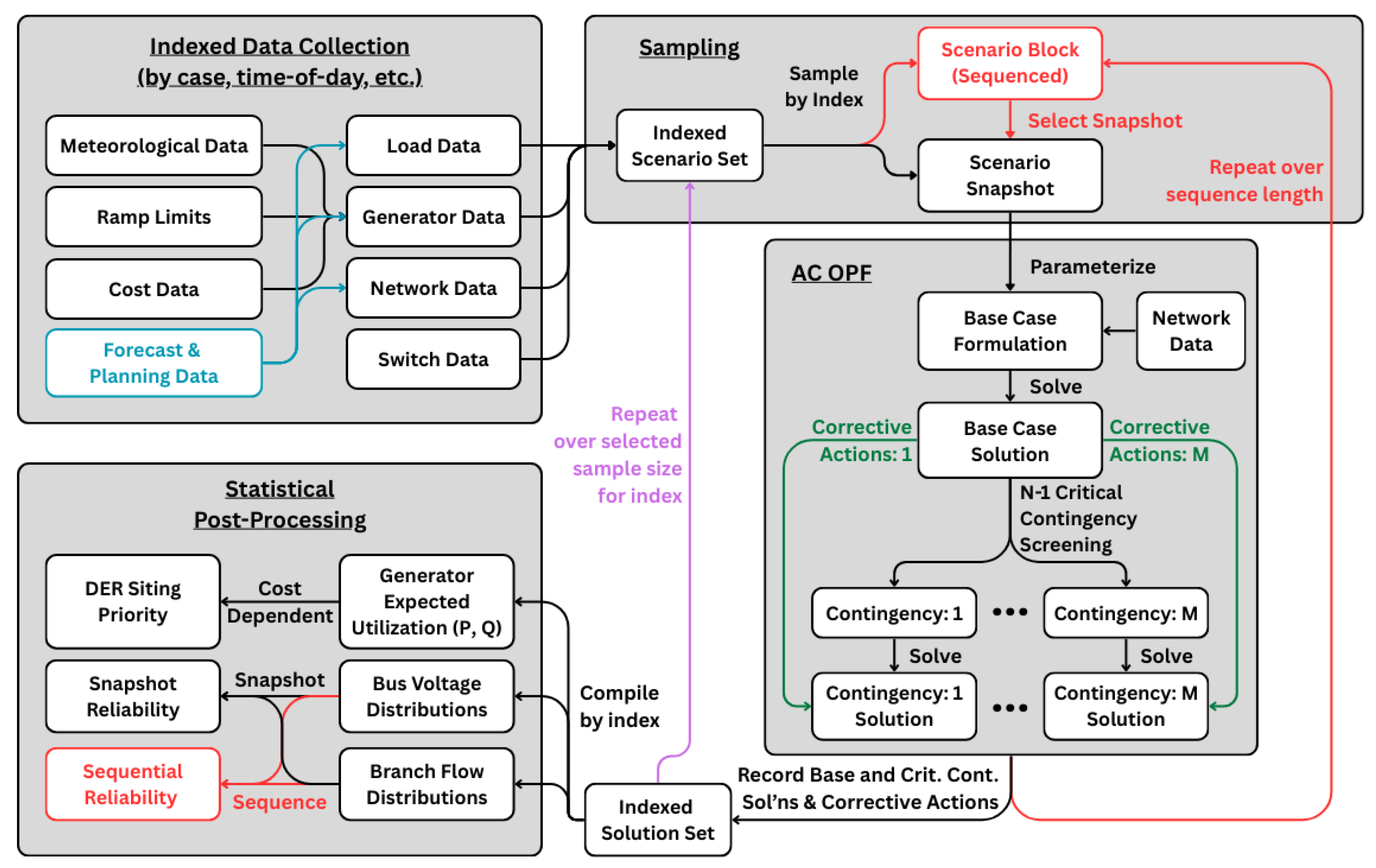
The Probabilistic Deliverability Assessment (PDA) framework presented here formulates an AC SBO workflow, as introduced in Section 3.4. System scenarios are sampled across a diverse range of load, resource, and contingency conditions. We show how both snapshot-based and time-sequential assessments can be performed by solving linked sets of parameterized AC OPF problems and aggregating the results into probabilistic metrics with confidence intervals.
The methodology assumes access to an AC OPF solver and focuses on the supporting data structures, scenario design, and workflow organization needed for probabilistic analysis in an interconnection study context. The process consists of four key components:
  • Indexed Data Collection: Input data, including network data, bus loads, generator capabilities, cost assumptions, switch states, voltage limits, and possible planning and forecasted assumptions, are compiled into an indexed scenario set, defined as a structured collection of time- or condition-specific scenarios.
  • Scenario Set Definition and Sampling: Individual scenarios or scenario blocks (sequences of scenarios) are sampled from the indexed set. Each scenario defines a complete operating condition to be evaluated, including DER limits, network topology, and costs. Sampling can be repeated over a selected sample size per index.
  • AC OPF Base Case and Contingency Evaluation: Data from each sampled scenario are used to parameterize AC OPF problems, solved to determine a feasible base dispatch. N-1 contingency screening is then applied to identify critical contingencies with limit violations, which are then re-solved with ramping constraints and control adjustments. Post-contingency solutions are recorded, including infeasible solutions.
  • Post-Processing and Statistical Interpretation: Indexed scenario outcomes are compiled to produce aggregated metrics, including DER expected utilization (active and reactive power), deliverability, and reliability estimates for cases and time blocks.
An overview of the methodology is shown in Figure 2. At a high level, the diagram illustrates the process flow, including data handling through repeated scenario sampling, AC OPF evaluation, contingency handling, and post-processing.
The process is designed to accommodate varying data granularity, enabling PDAs under both static and time-dependent operating conditions. We explore each process block in detail in the subsections to follow.

4.1. Scenario Sets and Sampling

To construct scenarios for evaluating candidate DERs under diverse operating conditions, we begin by defining a global scenario space that contains all available parameterizations of system data. This space forms a “structured bag” of load profiles, generation capabilities, network configurations, and cost parameters from which snapshots or blocks are later drawn. Formally, let
S : = D × G lim × E × C ,
where
  • D is the set of all candidate load data across injections (e.g., representative demand cases, historical or synthetic time series, or distributional models);
  • G lim is the set of generator or DER capability data (e.g., output bounds, ramp limits, or stochastic availability models);
  • E is the set of network configurations (e.g., feasible switch states or tap positions);
  • C is the set of cost parameters (e.g., linear, piecewise, or quadratic cost curves, possibly varying by regime).
A generic element of S is a tuple ( D , G , E , C ) with D D , G G lim , E E , C C . Not every such combination is meaningful; for example, a nighttime load profile should not be combined with daytime PV generation limits, and a summer cost regime may be incompatible with winter demand.
To define admissibility and allow for indexing later on, we associate each data element with labels that describe its operating context. Formally, we introduce label maps
τ D : D K D , τ G : G lim K G , τ E : E K E , τ C : C K C ,
where K D , K G , K E , K C denote the label spaces for load, generation, network, and cost data, respectively. These label spaces may include attributes such as season, hour of day, weather regime, or unit commitment plan, depending on the data type. Each map τ assigns one or more labels to a data element. For example:
  • τ D ( D ) might label a load profile D D as “summer weekday, 18:00” or “winter weekend, 02:00”;
  • τ G ( G ) might label a generator capability curve G G lim with time of day and a UC plan ID or with a weather regime affecting renewable availability;
  • τ E ( E ) could label a network configuration E E as valid for a particular maintenance schedule or switching regime;
  • τ C ( C ) might label a cost function C C as belonging to a specific fuel price scenario or seasonal tariff structure.
In this way, labels provide the contextual information that allows us to decide which elements may be combined into admissible tuples. Keys can then be defined as subsets of label components drawn from these spaces, while rules provide a more general way to encode compatibility across them. We illustrate both approaches below.
  • Key-Based Admissibility
A straightforward way to define admissibility is by selecting subsets of labels from the component label spaces. For example, we may restrict load profiles to those tagged as “peak demand,” while allowing flexible generator limits and network configurations. In general, for a key k = ( k D , k G , k E , k C ) with k D K D , k G K G , etc., the admissible set is
S adm ( k ) = D ( k D ) × G lim ( k G ) × E ( k E ) × C ( k C ) ,
where, for instance, D ( k D ) D denotes all load elements whose labels lie in k D . Tuples are admissible whenever each component comes from the subset identified by the key. As an example, a key defined as “12:00 noon” may restrict load data to profiles tagged with that time across all seasons, while allowing any valid generator plan or network state. Alternatively, a key defined by a specific UC plan ID constrains generator data but does not affect load or network choices.
  • Rule-Based Admissibility
Key-based selection can be limiting when admissibility depends on relationships across label spaces. A more general approach is to define a compatibility rule ϕ : K D × K G × K E × K C { true , false } that evaluates whether a tuple of labels is valid. The admissible set is then
S adm = ( D , G , E , C ) S : ϕ ( τ D ( D ) , τ G ( G ) , τ E ( E ) , τ C ( C ) ) .
For example, a rule could permit generator limits tagged “13:00” to pair with load profiles tagged either “13:00” or “14:00,” capturing a tolerance around wind availability. Another rule could exclude certain cost curves whenever the network is labeled with a planned maintenance outage.
Key-based admissibility can thus be viewed as a special case of rule-based admissibility, where ϕ enforces membership in specified subsets. In practice, keys provide a simple, industry-aligned mechanism, while rules offer a more general abstraction. For the remainder of this paper, we refer simply to S adm as the admissible scenario space, regardless of how it is constructed.
  • Snapshots and Blocks
From the admissible space S adm , we construct two types of scenario objects: snapshots, which represent individual operating conditions, and blocks, which represent temporally ordered sequences of operating conditions. These objects form the basis for sampling realizations used to parameterize AC OPF problems.
  • Scenario Snapshots: For a given case or time index t T , let S t S adm denote the admissible snapshot set at index t, as defined by the chosen labels or rules. A realized snapshot for sample s is then S s , t = ( D s , t , G s , t lim , E s , t , C s , t ) S t .
  • Scenario Blocks: For an index interval T = { 1 , , T } , let S T S adm T denote the admissible block set, containing ordered sequences of snapshots that satisfy temporal consistency. A realized block for sample s is then S s , T = { S s , t } t = 1 T S T .
Blocks preserve both sequencing and inter-temporal dependencies such as ramping limits, unit commitment schedules, state-of-charge trajectories, and planned outages by enforcing coupling constraints across the sequence. When underlying data encode correlations beyond the block horizon, the admissible block set may be defined over a buffered index interval  T + = { τ past + 1 , , 0 , 1 , , T , T + 1 , , T + τ future } . Sampling is performed on T + to preserve statistical or physical dependencies, while OPF evaluation is carried out on the restricted interval T .
Labels and rules translate naturally into constraints on the index set T . For example, a label defined as “12:00 noon” generates snapshots at indices t corresponding to noon across different seasons. A rule might allow load profiles at t labeled “13:00” to pair with generation data labeled “14:00,” producing sequences that preserve realistic correlations in renewable availability. In this way, labels and rules provide the structure needed to define indexed subsets of admissible data, S t or S T , which in turn form the basis for realized scenario samples S s , t and S s , T . The following subsections illustrate how concrete sampling methods can be applied to generate such realizations under different types of available data and levels of granularity.

4.1.1. Load Modeling and Sampling: Representative Cases

System load is defined at the bus level for the AC OPF problem. For a given scenario snapshot S t , denote the active and reactive power demand at bus i as
D t ( i ) = P D , i , t , Q D , i , t .
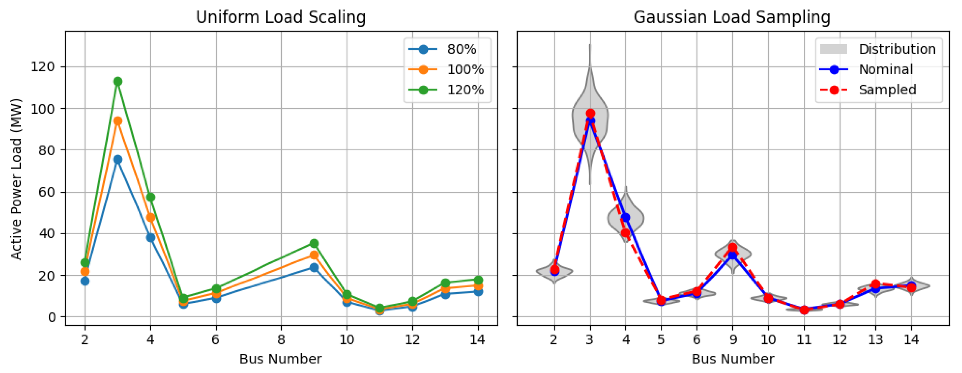
Load profiles drawn from peak or representative system conditions are suitable for stress testing but offer limited insight into the robustness of system performance near these points. To support broader assessment, we illustrate two methods for generating and sampling varied load conditions around a base case.
  • Uniform Scaling Based on Load Forecasts
Given a nominal load profile D t base , forecasted load growth or planning scenarios can be used to derive scaling factors α s to uniformly scale the base demand profile:
D s , t = α s · D t base , α s R + .
This simple approach preserves the spatial load distribution and is used for stress testing and in planning studies when only net demand projections are available.
  • Stochastic Perturbation of Per-Bus Loads
To introduce spatial diversity and stress test robustness around an operating point, the load at each bus can be independently sampled from normal distributions:
P D , i N ( μ i , σ i 2 ) , Q D , i N ( μ i , ( σ i ) 2 ) .
In this formulation, μ i and μ i denote the nominal active and reactive loads at bus i, while σ i and σ i capture their estimated variability. These variability estimates may be derived from historical load data or inferred from customer composition and behavior. This method supports the exploration of feasibility margins near constraint boundaries and enables the generation of statistically diverse loading scenarios for probabilistic assessment.
Figure 3 illustrates how each method can be applied to a small test system to explore system response under varying stress conditions.

4.1.2. Load Modeling and Sampling: Time Series Data

Time series data offer a rich foundation for constructing robust scenario sets that capture realistic temporal variability in system load. When available, these data support both raw and statistical sampling of hourly or sub-hourly load profiles, enabling analysis of intra-day dynamics, ramping behavior, and seasonal variation.
For use in a system model, the admissible load set D t D at index t must be instantiated by a realized profile D s , t . We illustrate two methods, raw sampling from data and distributional sampling, for generating and sampling load scenarios from time series data.
  • Raw Sampling
Using sufficiently long time series data, historical or synthetic time series can be parsed and collected into sets based on defined categories (e.g., summer weekdays and winter weekends). We can then, for example, randomly sample full-day profiles from which we can select specific hours or time blocks. This method preserves the temporal structure and correlations observed across hours.
  • Distributional Sampling
We can also use statistical properties computed across grouped time series to generate samples. As an example, we can parameterize a multivariate normal distribution by calculating the empirical mean vector and covariance matrix for hours in a day and generate scenario samples from this distribution. This method is well-suited for use cases where only aggregated statistics are available or where synthetic replication of typical patterns is needed across multiple sites.
Figure 4 visualizes both sampling approaches using summer weekday data compiled from CAISO hourly total load profiles [36]. Raw profile sampling preserves observed load patterns, while distributional sampling enables generation of statistically diverse scenarios.
Together, these methods support the construction of realized samples D s , t , which may appear either as single profiles in representative snapshots S s , t or as ordered sequences { D s , t } t T within time-sequenced scenarios S s , T , thereby reflecting real-world variability.

4.1.3. Generator Output and DER Representation

DER profiles, such as those from solar PV and wind, can be modeled as either fixed or variable injections, depending on data availability and system control. Below, we show how DERs can be modeled in OPF formulations, either as fixed passive injections or as actively controllable resources.
  • Fixed Injection (Negative Load Model)
In this approach, DERs are modeled as negative loads with fixed profiles, typically derived from historical data or simulations (e.g., PVsyst for solar). This representation is appropriate for behind-the-meter or non-dispatchable resources and is widely used in interconnection studies where DER control is not assumed. For a given generator at bus i at index t, we denote the feasible power limits as
G t ( i ) = ( P G , i , t min , P G , i , t max , Q G , i , t min , Q G , i , t max ) .
The realized generator limit profile for a realized sample s is then G s , t lim , which compactly represents the admissible ranges of active and reactive power for all generators under scenario sample S s , t .
  • Dispatchable DERs with Bounds
When modeling controllable DERs (e.g., utility-scale PV or wind with curtailment or hybrid control), upper and lower bounds can instead be used that reflect physical capabilities (e.g., irradiance limits or wind speed cutouts) as well as control settings.
To illustrate how to generate synthetic scenarios from real-world time series, we apply the same two approaches introduced in Section 4.1.2 to hourly profiles of solar and wind. Figure 5 illustrates both sampling modes for data on spring weekdays in 2019, compiled from ENTSO-E [37]. The top and bottom rows show solar and wind output, respectively.
The distributional sampling approach shown in the center panels uses a multivariate normal distribution parameterized by the empirical mean and covariance of the time series. However, it is important to assess the validity of the Gaussian assumption. In the case of wind, the output distribution is notably skewed, with many low-generation days and a few high-output outliers. This asymmetry leads the Gaussian model to overestimate output during several hours, particularly midday. When such skew is present, alternative models such as bootstrapping, empirical copulas, or bounded distributions (e.g., Beta) may better match the physical characteristics of the resource.

4.1.4. Switch States and Topology Variants

Power system topology can vary with the use of discrete control devices such as:
  • Circuit breakers, which isolate or energize transmission or distribution elements;
  • Tap changers, which adjust transformer voltage ratios in discrete steps;
  • Busbar or loop switches, which reconfigure live substation connectivity.
For a given index t, the admissible set of network configurations is denoted E t E , and a realized configuration for sample s is written as E s , t E t .
Scenario generation involving topology changes typically draws from a finite set of pre-screened configurations that are operationally valid and N-1-secure in the absence of candidate DERs. This avoids exploration of an intractable combinatorial space and maintains alignment with standard practices.
For tap changers specifically, their settings can sometimes be included as discrete decision variables within the AC optimal power flow (AC OPF) formulation. When permitted by the solver and model structure, tap positions can be co-optimized with generator dispatch to reduce losses, improve voltage profiles, and relieve network constraints.

4.1.5. Generator Cost Parameters

Generator costs are typically modeled using one of the following forms:
  • Linear: Constant marginal cost across all output levels.
  • Piecewise Linear: Stepwise approximation of a nonlinear cost curve.
  • Quadratic: Smooth cost function of the form C ( P ) = a P 2 + b P + c .
For a given index t, the admissible cost set is denoted C t C , and a realized sample for scenario s is written as C s , t C t . The vector C s , t may include coefficients ( a , b , c ) for quadratic models, slopes and breakpoints for piecewise linear models, or marginal costs for linear models.
For existing generators, cost models can be derived from historical bid data, heat rate curves, or assumed marginal costs. For candidate DERs, however, the modeling choice impacts insights gained for feasibility screening.
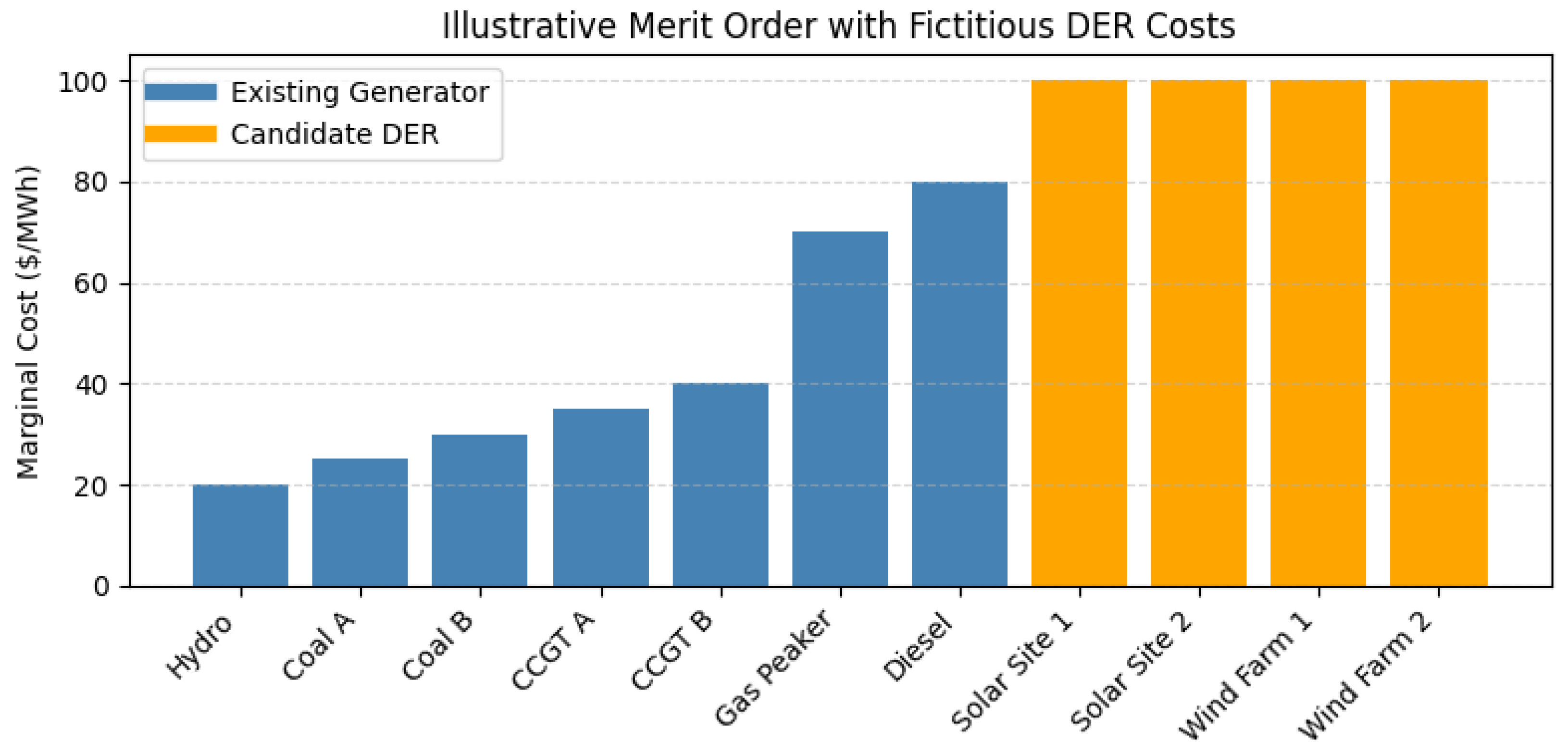
The conventional approach assigns near-zero marginal costs to candidate renewable DERs (e.g., wind and solar), causing them to be preferentially dispatched in economic dispatch formulations. While this reflects typical market behavior, it obscures whether the candidate’s output is preferential given physical system constraints.
  • Candidate Reserve Cost Structure
We propose an alternative structure in which all candidate DERs are assigned a uniform, fictitiously high marginal cost, higher than that of any existing generator over its operating range. This ensures existing generators are dispatched first and candidate DERs are only dispatched when required to meet demand under the AC power flow constraints.
Let G existing G denote the set of existing generators as a subset of all generators in a network and let G DER G denote the set of candidate DERs under evaluation. We can then express the cost function to show the separation between existing and candidate generators as follows:
min P G i G existing C i P G , i + j G DER C D E R fictitious P G , j .
In this formulation, candidate DERs act as high-cost reserves. The fictitiously high marginal cost is a modeling construct introduced to isolate feasibility-driven dispatch from economic behavior. This ensures that candidate DERs are dispatched only when required by AC network constraints, so their utilization reflects physical deliverability under system conditions rather than merit order economics. Figure 6 illustrates this separation using linear cost models.

4.2. Base Case AC OPF Formulation

We formulate base case AC OPF problems as nonlinear programs that minimize total generation cost subject to network physics and operational constraints. This standard formulation captures a single steady-state operating point, parameterized by scenario-specific inputs for load, generation, cost, and network configuration.
Let N be the set of buses, G the set of generators, and  L the set of lines and transformers, all of which are part of the fixed system definition. Scenario-dependent quantities such as load profiles, generator limits, cost parameters, and topology states are drawn from the realized datasets D s , t , G s , t lim , C s , t , and E s , t defined earlier. The decision variables include active and reactive generator outputs, voltage magnitudes, and voltage angles. The base case AC OPF is expressed as follows:
min P G , Q G , V , θ i G C i P G , i ,
subject to P G , i P D , i = V i j N V j ( G i j cos θ i j + B i j sin θ i j ) , i N ,
Q G , i Q D , i = V i j N V j ( G i j sin θ i j B i j cos θ i j ) , i N ,
P G , i min P G , i P G , i max , i G ,
Q G , i min Q G , i Q G , i max , i G ,
V i min V i V i max , i N ,
S i j ( V , θ ) S i j max , ( i , j ) L .
Here, P G , i , Q G , i are generator injections, P D , i , Q D , i are demands, V i is the voltage magnitude, θ i j = θ i θ j is the angle difference across buses, G i j + j B i j represents branch admittances, and  S i j denotes the apparent power flow magnitude on line ( i , j ) . Superscripts “min” and “max” denote lower and upper limits, respectively.
  • Fixed System vs. Scenario Data
Fully specifying this model requires both fixed system data and scenario-specific realizations. The fixed network model includes bus, generator, and line sets ( N , G , L ) , along with line parameters (impedances, shunts, and thermal ratings S i j max ) and per-bus voltage limits. Scenario-dependent inputs are drawn from the realized datasets: load profiles D s , t , generator capability limits G s , t lim , cost parameters C s , t , and network configurations E s , t . We present this division between fixed and scenario-dependent data as standard, but it can be adjusted as needed. For example, certain loads may be modeled as controllable or sheddable, and dynamic line ratings may be incorporated as part of the scenario realization.
  • Treatment of DERs
Controllable DERs (e.g., utility-scale PV or wind with curtailment or hybrid sites) can be included in G , with bounds specified in the realized limit profile G s , t lim . Non-dispatchable DERs (e.g., rooftop PV) can be modeled as negative injections within the realized load profile D s , t . Candidate DERs can be assigned fictitious costs through the realized cost vector C s , t , as described in Section 4.1.5, ensuring they are dispatched only when required by system conditions.

4.3. Contingency Screening and Corrective Dispatch

To improve tractability when solving many scenarios, we adopt a two-stage N-1 contingency evaluation. In the first stage, a fast linearized screen identifies which single-component outages may violate operating constraints. In the second, only these critical contingencies are re-solved using full AC OPF to determine corrective dispatch.
  • Contingency Screening via Linearized Jacobian
The screening stage uses the Jacobian matrix evaluated at the base case to approximate system response. For each contingency, we compute changes in active and reactive power injections ( Δ P , Δ Q ) at affected buses based on bus, generator, and branch (line or transformer) disconnects. We then approximate the resulting voltage magnitude and angle deviations ( Δ V , Δ θ ) as follows:
Δ θ Δ V = J 1 Δ P Δ Q ,
where J is the Jacobian of the power flow equations at the base operating point. These linearized deviations are used to estimate post-contingency flows and voltages. If any constraint is violated, the contingency is marked as critical.
  • Corrective Dispatch Formulation
For each critical contingency c, the AC OPF is re-solved with an updated topology and component status. Control actions such as generator re-dispatch, DER adjustments, and storage charge/discharge are permitted within operating bounds.
Let x 0 denote the base case dispatch and x c the corrected dispatch under contingency c. The corrective OPF is written as follows:
min x c C ( x c ) s . t . h c ( x c ) = 0 , g c ( x c ) 0 , x c F c ( x 0 ) ,
where h c ( · ) and g c ( · ) represent the AC power flow and operating constraints under contingency c, and  F c ( x 0 ) defines the feasible adjustment region around the base solution x 0 (e.g., due to ramping and reserve limits).
  • Inclusion of Infeasible Solutions
If no feasible re-dispatch x c exists, we record the least violating solution by applying controlled relaxations to binding constraints, including implementing emergency voltage limits (typically ± 10 % ) instead of nominal voltage limits (typically ± 5 % ) or substituting Rate B/C thermal ratings for Rate A limits. These cases flag where corrective actions are insufficient and infrastructure upgrades or revised base case assumptions may be needed.

4.4. Snapshot and Sequential Scenario Handling

The proposed framework accommodates two classes of scenario structures: case-based (snapshot) scenarios, which are independent, and block (sequential) scenarios, which evolve over time. Both are compatible with the core procedure for deliverability assessment.
  • Case-Based (Snapshot) Scenario Handling
With case-based scenarios, each scenario represents a fully parameterized AC OPF problem for a given case study. These snapshots are independently solved; there is no temporal dependency or cross-scenario interaction, except for optimal control actions linking base case solutions to post-contingency solutions. This formulation aligns with typical deliverability screening practices.
  • Block (Sequential) Scenario Handling
When time series data or forecast trajectories are available, scenarios can be structured as sequential blocks { S s , t } , where s { 1 , S } indexes sampled scenarios and t { 1 , T } indexes timesteps. In this mode, base case AC OPF problems are linked through inter-temporal constraints such as generator ramp limits, energy storage dynamics, or other state-coupled equations.
  • Contingency Evaluation Across Structures
Figure 7 gives an overview of how individual problem formulations are linked for both case-based and block scenarios. In both instances, N-1 contingency screening and corrective re-dispatch (as described in Section 4.3) are performed on each base case solution. For block scenarios, post-contingency states are not propagated forward in time. This design choice limits scenario tree branching and increases tractability for large networks and longer time horizons.

4.5. Post-Processing and Probabilistic Interpretation

Post-processing transforms raw OPF outcomes into interpretable metrics for reliability and resource utilization under uncertainty. We introduce a set of probabilistic metrics to support scenario-based evaluation.
  • Scenario-Based Reliability Estimation
For each scenario S s , t with sampling index s at case or time t, we assign the following binary feasibility indicator:
R s , t = 1 , if all constraints ( including contingencies ) are satisfied , 0 , otherwise .
We then define the probability of reliable operation at t as follows:
P ^ reliable ( t ) = 1 N t i = 1 N t R s , t ,
where N t = s = 1 S t ( 1 + M s , t ) is the number of scenarios evaluated at t across samples s 1 , , S t and contingencies per sample, with  M s , t as the number of contingencies for base scenario S s , t .
  • Time Block Reliability Estimation
In sequential simulations, we define the probability of reliable operation over a time block, T = { 1 , , T } , as the joint feasibility across all timesteps and contingencies in that block. Across the set of scenarios, S s , T , sampled with index s, we define
R s , T = 1 , if all OPF solutions in T are feasible , 0 , otherwise .
The time block reliability is then estimated by
P ^ reliable ( T ) = 1 S s = 1 S R s , T .
where S is the total number of samples taken.
This formulation requires joint feasibility across the entire interval, and is intentionally conservative: any single infeasible timestep or contingency causes the entire block to be marked as infeasible. Users seeking a less stringent metric may instead apply the scenario reliability estimate over each t T and aggregate the results.
Together, these metrics enables easily interpretable summary statements, such as “The reliability of simulated dispatch including candidate sites was 98% from 9:00 to 17:00,” or “The reliability of dispatch under peak demand with candidate DERs was 75%.”
  • Confidence Intervals for Reliability Estimates
The empirical reliability estimate P ^ reliable ( t ) represents the fraction of scenarios at time t that are feasible under both base and contingency conditions. It can be interpreted as the maximum likelihood estimator (MLE) of the underlying probability that a randomly drawn scenario is feasible under the simplifying assumption that scenario outcomes are independent Bernoulli trials. To quantify uncertainty in these estimates, a normal approximation confidence interval is used. At case or time t,
P ^ reliable ( t ) ± z α / 2 P ^ reliable ( t ) ( 1 P ^ reliable ( t ) ) N t ,
where z α / 2 is the critical value of the standard normal distribution for the desired confidence level (e.g., 1.96 for 95% confidence interval).
This formulation assumes scenario outcomes are independent, which is not strictly true given how scenarios are linked. In the case-based formulation, contingency outcomes share a common base dispatch, introducing within-sample dependence. In the sequential formulation, inter-temporal coupling (e.g., ramp limits and state-of-charge constraints) introduces dependence across timesteps. As a result, the variance of P ^ reliable may be underestimated, and reported confidence intervals may be narrower than nominal.
Nonetheless, under typical transmission planning and resource adequacy practices, base case scenarios are designed to be solvable and N-1-secure. Infeasibility is therefore expected to arise primarily in contingency evaluations, which are not propagated forward to other scenarios. Furthermore, there is no cross-sample dependence across base scenarios at the same timestep. When candidate DERs follow a candidate reserve cost structure (see Section 4.1.5), existing firm generation is prioritized, reducing the likelihood of structural infeasibility in later sequential scenarios. These considerations limit the degree of practical scenario dependence and support the interpretation of the confidence intervals as reasonable approximations. For these reasons, we report the standard interval form here and do not pursue variance corrections or sampling refinements.
Lastly, we note that time block reliability estimates, R s , T , are independent across sampled blocks, and the estimator P ^ reliable ( T ) satisfies the standard assumptions of the binomial model. As such, its confidence intervals can be interpreted without correction, providing a robust probabilistic statement about system-wide performance over time.
  • Expected Utilization and DER Deliverability
To quantify how much a controllable resource contributes across scenarios, we define its expected active power injection as follows:
E [ P G , i ] = 1 S T s = 1 S t = 1 T P G , i , s , t ,
where P G , i , s , t is the power output of generator G i in scenario S s , t , and S and T denote the number of sampled scenarios and cases or times considered in this estimate, respectively.
The per unit expected utilization is then
U G , i = E [ P G , i ] P ¯ G , i .
When the candidate reserve cost structure is used (as described in Section 4.1.5), the dispatch of candidate DERs is governed entirely by physical feasibility rather than cost-based merit order. In this context, U G can be interpreted as a deliverability metric, showing how much output from a DER is preferential, given network conditions and existing infrastructure constraints.
  • Visualization and Interpretation
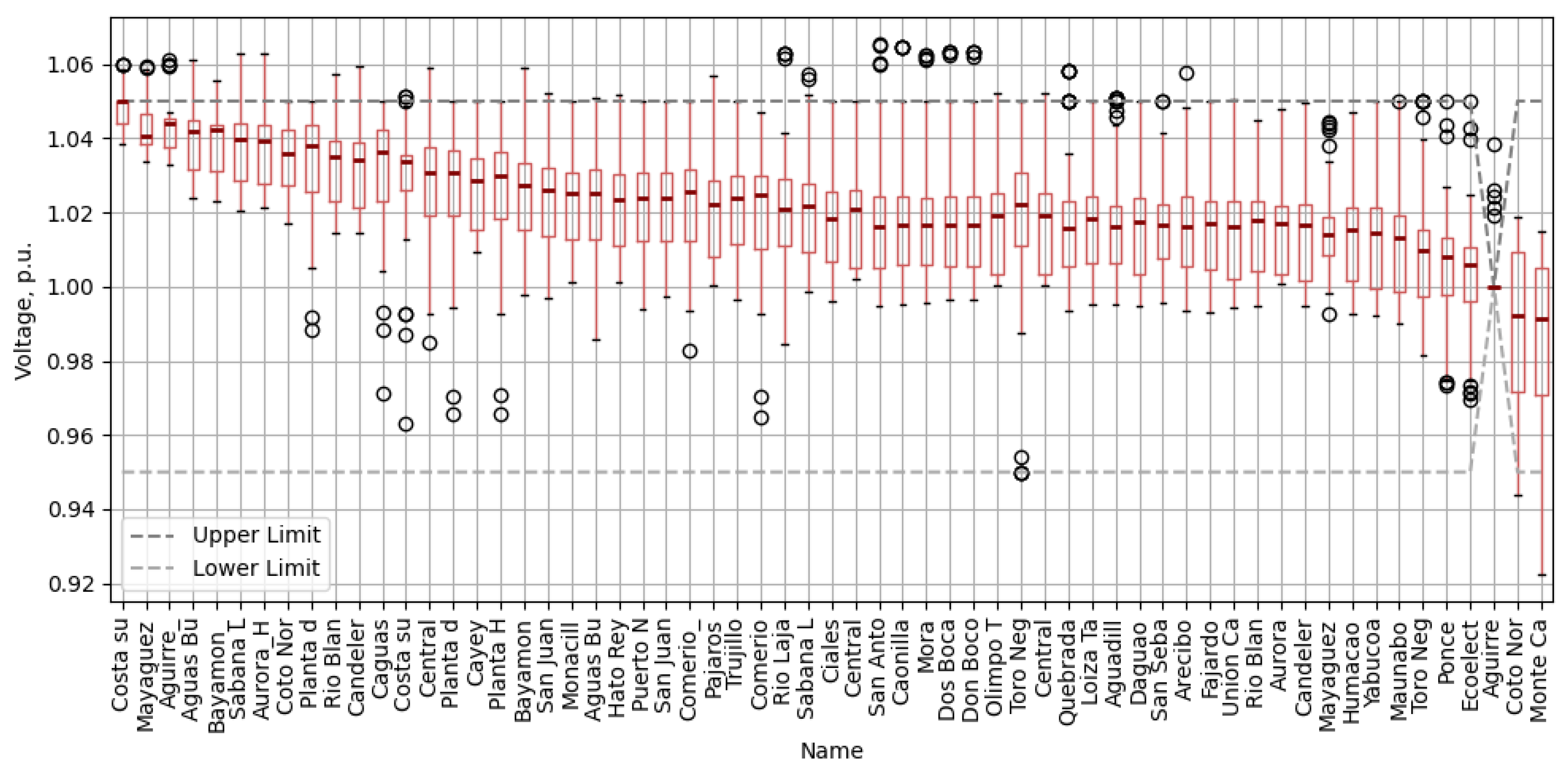
Aggregated metrics can be visualized through time series plots (e.g., reliability over time), performance profiles (e.g., bus voltages and limits), or spatial maps when combined with geographic data. For example, the following approaches can be used:
  • Bus voltage profiles can show how often solutions remain within limits, and outliers.
  • DER expected utilization and geospatial data can identify high-impact siting locations.
  • Tables can report per-component loading statistics against limits or summarize optimal corrective actions for contingencies for detailed review.
This post-processing framework transforms raw OPF outputs into actionable reliability insights and DER prioritization metrics, enabling both technical interpretation and policy-relevant decision-making.

5. Case Study: Advancing Decarbonization Efforts in Puerto Rico via Deliverability-Informed Hybrid Solar Siting

To demonstrate how the methodology in Section 4 can support site evaluations for interconnection and planning, we present a simplified case study of Puerto Rico’s bulk power system (BPS), expanded from [38]. This example illustrates how even a minimal-data, case-based scenario analysis—consistent with current interconnection study practices—can yield actionable insights by evaluating the deliverability of candidate DERs in clusters.
In the case study, we use an AC OPF solver from SmartGridz capable of handling various AC OPF formulations, including demand-side optimization. The SmartGridz solver can optimize settings for generators, transformers, shunts, adjustable loads, and DC lines, including voltage setpoints, while satisfying all system constraints [39].
The goal is to demonstrate how the proposed framework can complement and extend traditional cluster study processes, while motivating a shift toward more comprehensive time series-based scenario modeling in the future.

5.1. System Overview: Puerto Rican Public Grid Model

We utilize a 385-bus power flow model of Puerto Rico’s 115 kV and 230 kV BPS, derived from public data sources [40], with minor modifications to limits, setpoints, and branch impedances. The model also includes a 38 kV approximation of the subtransmission system, constructed via Kron reduction. This layer is represented as a fully connected subgraph with fictitious lines and approximate impedances. Violations and contingencies are restricted to the higher-level 115/230 kV BPS. Puerto Rico’s grid serves approximately 3 million residents and is structured as a meshed transmission network with radial distribution feeders [41]. Major load centers include San Juan, Ponce, Mayagüez, Arecibo, and Caguas, with generation primarily supplied by legacy oil-, diesel-, and gas-fired plants located near coastal ports. The grid’s 220 kV and 115 kV transmission corridors span the island, with bulk power typically flowing northward across the mountainous interior. Figure 8 illustrates the BPS infrastructure and major generating facilities.
To simulate DER integration under decarbonization scenarios, we consider load and resource portfolio projections from the Puerto Rico 100 (PR100) study [42] and scheduled asset retirements from the Puerto Rico Electric Power Authority (PREPA)’s 10-Year Plan [43]. Scheduled retirements include oil-fired units at San Juan, Palo Seco, and Aguirre within five years, AES coal by 2027, and Aguirre diesel units by 2030. PREPA’s Renewable Portfolio Standard (RPS) targets 40% renewable generation by 2025, 60% by 2040, and 100% by 2050, primarily through third-party DER deployments. The PR100 study confirms that these targets are technically feasible with sufficient solar and battery investments but leaves open questions regarding optimal siting, project sizing, and deployment timing.

5.2. Candidate DER Selection: Hybrid Solar Facilities

A notable takeaway from the PR100 study is the prevalence of solar PV and battery energy storage in generation mixes across planning scenarios. The large reliance on solar and batteries, combined with significant curtailment levels, motivates the consideration of hybrid solar facilities with controllable active and reactive power output. To reflect realistic deployment potential, we follow NREL estimates [44], which identify over 2000 MW of solar potential across 56 municipalities in Puerto Rico.
Based on these findings, we consider 50 candidate hybrid solar DER sites on the 115 kV network, each with a nameplate capacity of 40 MW, totaling 2000 MW of candidate capacity. Sites are selected for geographic diversity and are assumed capable of reactive power support [45]. The decision to connect at the 115 kV level was a compromise, balancing DER representation with overall model tractability.
Existing generation assets are assigned linear marginal costs based on the 2019 Siemens Integrated Resource Plan (IRP) [46], with the highest cost asset (AES coal) priced at USD 36/MWh. All candidate DERs are modeled as dispatchable and are configured as reserve units with a fictitious marginal cost of USD 100/MWh. This setup ensures dispatch priority remains on legacy resources and that only system constraints influence DER dispatch.

5.3. Scenario Definition: Retirement Stages, Contingencies, and Load Forecasts

In this case study, we define cases based on staged retirements of major generation assets in order to index scenarios. For each retirement stage, we evaluate multiple load levels and assess performance under both base and contingency conditions. The scenario design is summarized below.
  • Retirement Stages: Four sequential retirement stages are modeled based on PREPA’s published schedule. While the original plan retires individual generating units, the model used here aggregates each plant as a single generator. As such, entire facilities are retired at each stage to reflect unit-level retirements within the available modeling fidelity:
    • No retirements;
    • Retirement of all San Juan assets;
    • Additional retirement of Palo Seco assets;
    • Additional retirement of all Aguirre assets.
  • Contingency Analysis: For each scenario, we evaluate the base case, perform N-1 contingency screening, and simulate selected critical contingencies to assess feasibility under stress conditions. While optimal corrective actions are computed, they are omitted here for brevity; see [38] for details.
  • Load Scenarios: We model three load levels around a peak loading scenario, scaled to 80%, 100%, and 120% of the public model’s base demand, reflecting the deployment scenarios outlined in PR100.

5.4. Results: Computation Time

On the system model used here (385 buses, 62 generators), individual AC OPF scenarios were solved in 1–3 s on a laptop with an Intel i9-12900H CPU and 32 GB RAM. Failed runs, when they occurred, typically terminated within 2–4 s.
We therefore estimate that the full 72-scenario case was completed within several minutes of wall-clock time, with manual adjustments between cases taking far longer than solver execution. Comparable studies on a proprietary model of the Puerto Rico bulk power system (∼1400-buses), maintained by LUMA Energy, reported similarly tractable runtimes [47].

5.5. Results: Case Reliability Estimates

Figure 9 and Figure 10 summarize bus voltage and line flow statistics across all scenarios and retirement stages. Mean bus voltage magnitudes remain within ± 5 % of nominal across the BPS, with only a few minor relaxations (within ± 10 % ) observed during select N-1 contingencies. Line flows remain within Rate A limits across all cases. These results confirm that the majority of scenarios are feasible, and violations, when they occur, are marginal (under 2%). Moreover, the few recurring violations tend to localize around specific buses, indicating where targeted upgrades may yield the greatest benefit.
We also estimate the scenario-based reliability outlined in Section 4.5 for each stage of retirement and overall. These are summarized in Table 1.

5.6. Results: DER Expected Utilization and Deliverability

Figure 11 shows active power dispatch statistics for each candidate DER site under the final retirement stage. In [38], we present results for all four retirement stages and observe increased DER dispatch as legacy generation is retired, peaking in the final stage shown here. Because dispatch levels vary systematically across retirement stages, we compile dispatch statistics per stage rather than over all stages simultaneously.
Because candidate DERs are represented using the candidate reserve cost structure, their reported expected utilization is best understood as a deliverability indicator, showing where their output is physically accommodated under network constraints rather than selected through economic merit order. Figure 11 highlights the sites that provide the greatest system value on this basis, underscoring how the PDA framework can extract location-specific insights even in the absence of detailed time series data.
We extend these insights in Figure 12 by visualizing the expected utilization (in MW) of each candidate DER site geographically. Through this we see that the Humacao region has the highest utilization density, followed by the Vega Alta area. Interestingly, expected utilization within the capital area, San Juan, was distributed among numerous small facilities. While this was not planned for, it aligns well with the reduced capacities typically seen from rooftop PV installations. These insights show where it might be most useful to solicit requests for proposals (RFPs) for new facilities.

5.7. Results: DER Reactive Power and Grid Support Insights

In addition to active power dispatch, we assess the reactive power capabilities of the candidate DER sites. Many grid-forming inverters and hybrid solar systems are capable of supporting voltage regulation through dynamic reactive power injection or absorption [45]. Understanding which DER sites are most often called upon to provide reactive support can guide power purchase agreement (PPA) requirements and facility design, including voltage support equipment.
Figure 13 presents the average reactive power contributions from DERs across all base and contingency cases in the final retirement stage. These outcomes reveal several system-level insights. As legacy thermal units retire, the analysis highlights specific areas where additional distributed reactive compensation becomes necessary for optimal dispatch. Much of this demand aligns with large load centers and industrial zones, consistent with significant inductive demand. When reactive injections coincide with active dispatch, hybrid PV–battery sites emerge as particularly valuable since they can manage both active and reactive power flexibly. In contrast, for PV-only facilities, developers may need to oversize nameplate capacity or install dedicated shunt banks, which is common practice at utility-scale plants. Finally, in locations where reactive power is dispatched without active output, the findings suggest a role for stand-alone compensation devices, either new shunt capacitors or conversion of retired synchronous machines into condensers. In Puerto Rico, this appears especially relevant around the San Juan metropolitan area.
Taken together, these metrics offer an interpretable way to differentiate DERs not just by generation potential but by their value to the system’s dynamic support needs under future retirement and loading conditions. This provides an additional layer of systems thinking to interconnection evaluation processes and could be used to differentiate numerous candidate facilities based on system needs. For planners and developers, this highlights candidate locations where investments in generation and reactive power capabilities may be most beneficial.

6. Discussion

This work addresses recognized limitations in current interconnection study practices, including reliance on fixed dispatch assumptions, limited scenario representation, and deterministic evaluation criteria. To address these shortcomings, we reviewed state-of-the-art approaches for embedding uncertainty into OPF formulations, including chance-constrained, stochastic, robust, and scenario-based methods, and found that a scenario-based OPF workflow provides the best balance between tractability, interpretability, and scalability. Building on this insight, we introduced the PDA framework, which formulates structured, SBO-based AC OPF problems. The framework accommodates operational variability, network constraints, and DER flexibility, factors that are often excluded or oversimplified in current modeling assumptions. In contrast to deterministic feasibility outcomes, it generates interpretable metrics such as expected DER utilization and probabilistic reliability. These outputs improve interconnection decision-making and inform broader planning efforts by enabling stakeholders to prioritize DER sites not only by feasibility but also by their expected contribution to system reliability and grid support.
In this section, we discuss modeling assumptions and limitations of the framework and case study, practical considerations for implementation, industry adaptation, and opportunities for future research before making concluding remarks.

6.1. Modeling Assumptions and Limitations

The SBO structure provides a tractable way to overcome limitations in current interconnection assessments by accounting for optimal dispatch across uncertain injections and contingencies. At the same time, this formulation does not guarantee a globally optimal solution across linked scenarios, whether over time horizons or across contingency sets. Each scenario is solved independently, which enables faster individual solutions and post hoc aggregation into planning metrics rather than optimization over the sum of scenario costs. When extended over time horizons, branching paths can also yield problematic dispatch trajectories if unit commitment plans and inter-temporal constraints are not properly incorporated. These trade-offs distinguish the PDA framework as a planning and screening tool rather than an operational dispatch model, the latter being more appropriately addressed by formulations such as S-OPF. The strength of the SBO approach lies in its ability to generate ensembles of feasible solutions that can be interpreted through probabilistic metrics for planning and decision-making.
For the case study, several simplifying assumptions shape both the modeling and the results. Violations and contingencies at the 38 kV subtransmission layer were omitted, as this layer was approximated by a fully connected Kron-reduced network with fictitious lines in the public data model. Large generating stations were modeled as single generators, whereas in practice multiple units exist that operate as distinct gensets. Candidate DERs were represented using a reserve cost structure, which isolates feasibility-driven dispatch and highlights siting locations that can be accommodated by the grid. In practice, however, economic dispatch is governed by market marginal costs. A natural follow-up would be to apply true cost data to a reduced set of candidate projects identified through deliverability screening to support financing assessments. The public data model also excluded small generators and non-controllable PV, both of which exist in Puerto Rico and could be modeled as additional controllable units or fixed injections. Finally, load inputs were derived from scaled peak profiles to mirror the minimal-data procedures of interconnection assessments. This design supports consistency with current practice but does not capture inter-temporal dynamics that require time series data, which are identified as a direction for future work. Despite these simplifications, this study illustrates the framework’s ability to produce actionable insights, including the identification of high-impact DER sites and regions where integrated reactive power compensation would enhance grid performance. Mapping expected utilization with geospatial data highlights priority areas where utilities may localize development incentives, while probabilistic reliability metrics help assess whether candidate sites meet minimum reliability thresholds or require further analysis.

6.2. Practical Considerations for Implementation

Practical implementation of the PDA workflow raises considerations related to operational realism, computational scaling, input quality, and sampling precision.
Operational realism determines which corrective actions are feasible within the post-contingency time window. Communication delays, control response times, and the coordination of many DERs all bound feasible re-dispatch and corrective control. These factors are system-specific and can be represented through scenario design and OPF parameterization; examples include ramp limits, reserve headroom, or inverter control characteristics. We note these considerations but do not elaborate further, as the specific parameterization of each is problem-dependent and outside the scope of this paper.
A second consideration is computational scaling. While runtime was not a limiting factor in the case study presented here, larger systems, richer contingency sets, or expanded scenario sampling will increase the computational burden. If runtime becomes prohibitive, approaches such as scenario reduction, importance sampling, and parallelization can help maintain tractability. Because interconnection and planning studies are performed offline rather than under real-time dispatch deadlines, runtimes on the order of seconds per scenario remain tractable in practice. In this context, the more significant challenge is workflow integration and data availability rather than solver performance itself.
Third, the granularity and realism of input data strongly influence the reliability and interpretability of results. Full-year 8760-hour datasets can support daily blocks that capture diurnal variability, while longer blocks such as week-long sequences may be valuable in studies that explicitly consider medium-term storage feasibility. The representativeness of renewable profiles, spatial correlation of weather, credible contingency lists, and accurate DER parameters such as reactive power capability, ramp rates, and control modes are all material. Sensitivity analyses that vary these inputs within plausible ranges can reveal which assumptions most affect reported metrics.
Finally, the scale of sampling is an important consideration. The expected values of the reliability estimates reported here are determined by the system and therefore do not depend on the number of sampled scenarios, although the width of the associated confidence intervals does. For example, in Table 1, the 95% confidence interval half-width scales as O ( 1 / N t ) under the binomial model in (31). Increasing the number of scenarios tenfold, for example from N t = 18 to N t = 180 per stage, would reduce the half-widths by 1 / 10 , tightening from ± 0.1058 (R1/R2) to ± 0.0335 , and from ± 0.1452 (R3) to ± 0.0459 , while leaving the mean reliability unchanged. Practitioners can thus use (31) to size scenario sets to a target precision that matches study objectives.
We lastly acknowledge that solver robustness and software choice remain important in practice but note that they are not the focus of this paper. What is more relevant are considerations for reproducibility. Results can depend on solver choice and settings, so documenting solver versions, tolerances, and initialization strategies, fixing random seeds for sampling, and maintaining an audit trail that links plotted metrics to the underlying scenario inputs all improve transparency. When feasible, cross-validating a subset of cases with an alternative solver can provide additional assurance. Such practices are essential for building trust in PDAs and also support the institutional acceptance of these methods.

6.3. Considerations for Industry Adaptation

The PDA framework is designed to both complement and extend existing interconnection practices. In its simplest form, OPF formulations can be constrained to replicate traditional case-based power flow studies. This is a feature in SmartGridz, which allows OPF problems to be framed as fixed-dispatch power flow problems while also providing additional information through primal and dual solutions [39]. This ensures direct compatibility with current processes while enabling a gradual pathway toward more advanced assessments. The PDA framework is modular, allowing adoption to begin with optimal dispatch over snapshot-based cluster studies that reflect today’s workflows and extend to block-based or time-sequenced evaluations as data and modeling standards evolve. The use of AC OPF further enables integration of both preventive and corrective dispatch and can evolve with best practices in different operating territories. The framework represents a gradual paradigm shift: from static, case-based interconnection assessments to probabilistic insights drawn from large sets of optimal dispatch solutions over representative time blocks. Importantly, this shift can occur incrementally, enabling regulators and utilities to adopt the level of complexity most appropriate for their available resources and institutional needs.
For regulators and utilities, a central advantage of PDA is nuance and transparency. Traditional pass/fail interconnection outcomes obscure how often candidate projects are deliverable under realistic operating conditions. In contrast, PDA produces reproducible metrics such as expected utilization, probabilistic reliability with confidence intervals, and geospatial overlays of system needs. These outputs provide a more nuanced basis for ranking and evaluating multiple projects within a queue or cluster. Transparency is achieved by ensuring that different stages of the workflow can be delegated across teams and offices (such as data collection and preparation, solver setup and execution, and post hoc analysis and interpretation) and by making default datasets and assumptions open access so that applicants can assess whether these align with their projects or need to be customized. Documenting solver settings, random seeds, and scenario definitions further ensures that results are traceable and auditable, which is critical for regulatory acceptance and dispute resolution. Such reproducibility practices build confidence that results are not artifacts of a particular solver or dataset but are robust under independent audits.
Finally, industry adoption will require a cultural shift in how interconnection results are interpreted. Current processes emphasize conservative deterministic feasibility, whereas PDA introduces probabilistic deliverability metrics that reflect system variability and flexibility. Training analysts and stakeholders to interpret distributions and confidence intervals rather than deterministic outcomes will be essential. At its core, the approach substitutes fixed-dispatch AC power flow with AC OPF formulations that capture optimal dispatch under uncertainty, while preserving the ability to recover traditional case-based studies as a limiting form. In this way, PDA enhances existing procedures without disrupting regulatory compliance, offering a practical pathway for institutional adoption that can scale in complexity as data and modeling practices evolve.

6.4. Opportunities for Future Research

Future work can extend both the case study applications of the PDA framework and the framework itself. For the case study presented here, several directions are promising. A natural next step is to apply the workflow to larger systems and sampling sets. Study [47] demonstrates the tractability of solving the real ∼1400-bus Puerto Rico system with the same solver used here, making this a logical candidate for follow-on analysis. Open access benchmark networks such as the PEGASE models referenced in Section 3 also provide an opportunity for reproducible large-scale testing. Another important direction is expanding the temporal scope. For example, capturing diurnal variability for solar via daily blocks is compelling, and assessing energy adequacy and the need for medium-term storage using multi-day or week-long blocks is also possible within the framework. Larger scenario sets can also be employed to quantify how probabilistic deliverability estimates converge and how many samples are needed for acceptably narrow confidence intervals in practice. Finally, comparative studies across different jurisdictions or market contexts would help assess the portability of the PDA approach beyond the Puerto Rico system.
Future research for improving the PDA framework can weave elements of other OPF formulations into the SBO workflow. Robustness requirements could be included by jointly solving base case and contingency scenarios. Sequential stochastic OPF could be used to couple multiple time blocks, allowing inter-temporal constraints such as ramping and storage dynamics to be represented explicitly. Chance-constrained formulations could also replace hard feasibility requirements, enabling risk-aware deliverability assessments. More broadly, where multiple scenarios are solved together, indexing could be defined across the larger joint problem rather than at the level of independent operating points. Each of these directions would expand the applicability of PDA while preserving the modular, scenario-based structure.
Beyond specific case studies and formulations, opportunities also exist to improve the overall workflow. Automating the full pipeline of scenario sampling, parameterization, solving, and post hoc analysis would facilitate scaling to large interconnection queues and complex study designs. Cloud-based or high-performance computing environments could be leveraged for national-scale applications. Standardized input datasets, DER parameter libraries, and reproducibility templates would help establish PDA as a transparent and verifiable tool for industry and academic users alike. Ultimately, these extensions would broaden the applicability of PDAs and strengthen their role as a bridge between advanced OPF formulations and evolving interconnection practices.

6.5. Conclusions

This paper reviewed current industry practices and identified key modeling limitations. We then surveyed state-of-the-art approaches for handling uncertainty, motivating the choice of a scenario-based OPF (SBO) workflow. Building on this foundation, we developed a Probabilistic Deliverability Assessment (PDA) framework that embeds AC OPF formulations within structured scenario sets. The framework captures operational variability through scenario sampling, represents DERs with bounded dispatch variables, enforces security constraints via contingency screening and corrective actions, and aggregates indexed solution sets into interpretable outputs such as expected utilization and probabilistic reliability. In doing so, PDA addresses the shortcomings of current interconnection assessments, which rely heavily on fixed assumptions and deterministic feasibility outcomes. A case study on Puerto Rico’s bulk power system demonstrated that even a minimal-data implementation can uncover actionable siting insights for candidate hybrid solar projects and highlight locations where reactive power support is needed.
Looking ahead, the PDA framework offers both a practical tool for today’s interconnection challenges and a foundation for continued methodological innovation. Its modular design enables incremental adoption by regulators, utilities, and developers, while its probabilistic outputs improve transparency and comparability across projects. By bridging advanced OPF formulations with industry workflows, PDA advances the goal of more efficient, transparent, and reliable integration of distributed energy resources and sets the stage for future research on larger systems, richer datasets, and hybrid formulations.

Author Contributions

Conceptualization, L.L.A. and M.D.I.; Methodology, L.L.A.; Software, M.D.I.; Validation, L.L.A.; Formal Analysis, L.L.A.; Investigation, L.L.A.; Resources, L.L.A.; Data Curation, L.L.A. and M.D.I.; Writing—Original Draft Preparation, L.L.A.; Writing—review and editing, L.L.A. and M.D.I.; Visualization, L.L.A.; Supervision, M.D.I.; Project Administration, M.D.I.; Funding Acquisition, M.D.I. All authors have read and agreed to the published version of the manuscript.

Funding

The initial research was supported by a collaborative project between the Massachusetts Institute of Technology (MIT) and Pacific Northwest National Laboratory (PNNL), entitled “Toward a Dynamic Monitoring and Decision Systems (DyMonDS) Framework for Resilient Electricity Services: Puerto Rico BPS Feasibility Study,” conducted under the guidance of Marcelo Elizondo (subcontract number 680381). The extension of this work, including the research and preparation of this publication was based (fully or partially) upon work supported by the U.S. Department of Energy’s Office of Energy Efficiency and Renewable Energy (EERE) under the Hydrogen Fuel Cell Technology Office, Award Number DE-EE0010724. This report was prepared as an account of work sponsored by an agency of the United States Government. Neither the United States Government nor any agency thereof, nor any of their employees, makes any warranty, express or implied, or assumes any legal liability or responsibility for the accuracy, completeness, or usefulness of any information, apparatus, product, or process disclosed, or represents that its use would not infringe privately owned rights. Reference herein to any specific commercial product, process, or service by trade name, trademark, manufacturer, or otherwise does not necessarily constitute or imply its endorsement, recommendation, or favoring by the United States Government or any agency thereof. The views and opinions of authors expressed herein do not necessarily state or reflect those of the United States Government or any agency thereof.

Data Availability Statement

The authors gratefully acknowledge the use of the publicly available Puerto Rico system described in [40]. The base power flow model showcased in the case study was is available in the following GitHub repository, under “MIT_Report_PartIII”: https://github.com/lauanton/puerto_rico_psse_public_data (accessed on 2 July 2024).

Acknowledgments

The authors gratefully acknowledge Marcelo Elizondo of PNNL for his guidance during the initial research phase. They also thank Rupamathi Jaddivada, Director of Innovation at SmartGridz, for her support and initial guidelines on using the SmartGridz AC optimal power flow solver.

Conflicts of Interest

The authors declare no conflicts of interest. The funders had no role in the design of the study; in the collection, analyses, or interpretation of data; in the writing of the manuscript; or in the decision to publish the results.

References

  1. Ayres, D.; Zamora, L. Renewable Power Generation Costs in 2023; Technical Report; International Renewable Energy Agency (IRENA): Abu Dhabi, United Arab Emirates, 2024; ISBN 978-92-9260-621-3. Available online: https://www.irena.org/-/media/Files/IRENA/Agency/Publication/2024/Sep/IRENA_Renewable_power_generation_costs_in_2023.pdf (accessed on 2 July 2024).
  2. Rand, J.; Mills, N.; Gorman, W.; Wiser, R.; Seel, J.; Mulvaney, J.K.; Jeong, S.; Kahrl, F. Queued Up: 2024 Edition, Characteristics of Power Plants Seeking Transmission Interconnection As of the End of 2023; Lawrence Berkeley National Laboratory: Berkeley, CA, USA, 2024. Available online: https://emp.lbl.gov/publications/queued-2024-edition-characteristics (accessed on 2 July 2024).
  3. PJM Interconnection. PJM Manual 14H: New Service Requests Cycle Process; Technical Report 14H; PJM Interconnection: Audubon, PA, USA, 2025; Available online: https://www.pjm.com/-/media/DotCom/documents/manuals/m14h.pdf (accessed on 2 July 2024).
  4. PJM Interconnection. PJM Manual 14B: PJM Region Transmission Planning Process; Technical Report 14B; PJM Interconnection: Audubon, PA, USA, 2024; Available online: https://www.pjm.com/-/media/DotCom/documents/manuals/m14b.pdf (accessed on 2 July 2024).
  5. ISO New England (ISO-NE). ISO New England Planning Procedure No. 5-6: Interconnection Planning Procedure for Generation and Elective Transmission Upgrades; Technical Report No. 5-6; ISO New England (ISO-NE): Holyoke, MA, USA, 2024; Available online: https://www.iso-ne.com/static-assets/documents/rules_proceds/isone_plan/pp05_6/pp5_6.pdf (accessed on 2 July 2024).
  6. Midcontinent Independent System Operator (MISO). Business Practices Manual Generator Interconnection; Technical Report BPM-015-r26; Midcontinent Independent System Operator (MISO): Carmel, IN, USA, 2023; Available online: https://cdn.misoenergy.org/20230918%20PAC%20Item%2002c%20BPM-015%20Generator%20Interconnection%20Queue%20Reform%20Redlines630228.pdf (accessed on 2 July 2024).
  7. Federal Energy Regulatory Commission (FERC). FERC Docket No. RM22-14-000; Order No. 2023: Improvements to Generator Interconnection Procedures and Agreements; Technical Report 0230728-3060; Federal Energy Regulatory Commission (FERC): Washington, DC, USA, 2023. Available online: https://www.ferc.gov/media/order-no-2023 (accessed on 2 July 2024).
  8. Federal Energy Regulatory Commission (FERC). FERC Docket No. RM22-14-001; Order No. 2023-A: Improvements to Generator Interconnection Procedures and Agreements; Technical Report; Federal Energy Regulatory Commission (FERC): Washington, DC, USA, 2024. Available online: https://www.ferc.gov/media/e1-rm22-14-001 (accessed on 2 July 2024).
  9. Federal Energy Regulatory Commission (FERC). Pro Forma Large Generator Interconnection Procedures (LGIP); Technical Report; Federal Energy Regulatory Commission (FERC): Washington, DC, USA, 2024. Available online: https://www.ferc.gov/media/pro-forma-lgip (accessed on 2 July 2024).
  10. Federal Energy Regulatory Commission (FERC). Pro Forma Small Generator Interconnection Procedures (SGIP); Technical Report; Federal Energy Regulatory Commission (FERC): Washington, DC, USA, 2024. Available online: https://www.ferc.gov/media/pro-forma-sgip (accessed on 2 July 2024).
  11. Ramadan, A.; Ebeed, M.; Kamel, S.; Abdelaziz, A.Y.; Haes Alhelou, H. Scenario-Based Stochastic Framework for Optimal Planning of Distribution Systems Including Renewable-Based DG Units. Sustainability 2021, 13, 3566. [Google Scholar] [CrossRef]
  12. Jain, A.K.; Horowitz, K.; Ding, F.; Sedzro, K.S.; Palmintier, B.; Mather, B.; Jain, H. Dynamic hosting capacity analysis for distributed photovoltaic resources—Framework and case study. Appl. Energy 2020, 280, 115633. [Google Scholar] [CrossRef]
  13. Roald, L.A.; Pozo, D.; Papavasiliou, A.; Molzahn, D.K.; Kazempour, J.; Conejo, A. Power systems optimization under uncertainty: A review of methods and applications. Electr. Power Syst. Res. 2023, 214, 108725. [Google Scholar] [CrossRef]
  14. Wang, Z.; Younesi, A.; Liu, M.V.; Guo, G.C.; Anderson, C.L. AC Optimal Power Flow in Power Systems with Renewable Energy Integration: A Review of Formulations and Case Studies. IEEE Access 2023, 11, 102681–102712. [Google Scholar] [CrossRef]
  15. IEEE Std 1547-2018 (Revision of IEEE Std 1547-2003); IEEE Standard for Interconnection and Interoperability of Distributed Energy Resources with Associated Electric Power Systems Interfaces. Institute of Electrical and Electronics Engineers (IEEE): New York, NY, USA, 2018; pp. 1–138. [CrossRef]
  16. Tang, X.; Guo, Z. Co-optimization of Active and Reactive Power in Flexible Distribution Networks. In Proceedings of the 2024 6th International Conference on Energy, Power and Grid (ICEPG), Guangzhou, China, 27–29 September 2024; pp. 766–769. [Google Scholar] [CrossRef]
  17. Valova, R.; Brown, G. Distributed energy resource interconnection: An overview of challenges and opportunities in the United States. Sol. Compass 2022, 2, 100021. [Google Scholar] [CrossRef]
  18. Esteban-Pérez, A.; Morales, J.M. Distributionally robust optimal power flow with contextual information. Eur. J. Oper. Res. 2023, 306, 1047–1058. [Google Scholar] [CrossRef]
  19. Grover-Silva, E.; Girard, R.; Kariniotakis, G. Multi-temporal optimal power flow for assessing the renewable generation hosting capacity of an active distribution system. In Proceedings of the 2016 IEEE/PES Transmission and Distribution Conference and Exposition (T&D), Dallas, TX, USA, 3–5 May 2016; pp. 1–5, ISSN 2160-8563. [Google Scholar] [CrossRef]
  20. Capitanescu, F.; Martinez Ramos, J.L.; Panciatici, P.; Kirschen, D.; Marano Marcolini, A.; Platbrood, L.; Wehenkel, L. State-of-the-art, challenges, and future trends in security constrained optimal power flow. Electr. Power Syst. Res. 2011, 81, 1731–1741. [Google Scholar] [CrossRef]
  21. Venzke, A.; Chatzivasileiadis, S. Convex Relaxations of Security Constrained AC Optimal Power Flow Under Uncertainty. In Proceedings of the 2018 Power Systems Computation Conference (PSCC), Dublin, Ireland, 11–15 June 2018; pp. 1–7. [Google Scholar] [CrossRef]
  22. Bienstock, D.; Chertkov, M.; Harnett, S. Chance-Constrained Optimal Power Flow: Risk-Aware Network Control under Uncertainty. SIAM Rev. 2014, 56, 461–495. [Google Scholar] [CrossRef]
  23. Dall’Anese, E.; Baker, K.; Summers, T. Chance-Constrained AC Optimal Power Flow for Distribution Systems with Renewables. IEEE Trans. Power Syst. 2017, 32, 3427–3438. [Google Scholar] [CrossRef]
  24. Lubin, M.; Dvorkin, Y.; Roald, L. Chance Constraints for Improving the Security of AC Optimal Power Flow. IEEE Trans. Power Syst. 2019, 34, 1908–1917. [Google Scholar] [CrossRef]
  25. Tang, K.; Dong, S.; Ma, X.; Lv, L.; Song, Y. Chance-Constrained Optimal Power Flow of Integrated Transmission and Distribution Networks with Limited Information Interaction. IEEE Trans. Smart Grid 2021, 12, 821–833. [Google Scholar] [CrossRef]
  26. Mezghani, I.; Misra, S.; Deka, D. Stochastic AC optimal power flow: A data-driven approach. Electr. Power Syst. Res. 2020, 189, 106567. [Google Scholar] [CrossRef]
  27. Grangereau, M.; van Ackooij, W.; Gaubert, S. Multi-stage Stochastic Alternating Current Optimal Power Flow with Storage: Bounding the Relaxation Gap. Electr. Power Syst. Res. 2022, 206, 107774. [Google Scholar] [CrossRef]
  28. Wu, Y.; Chen, Z.; Chen, R.; Chen, X.; Zhao, X.; Yuan, J.; Chen, Y. Stochastic optimization for joint energy-reserve dispatch considering uncertain carbon emission. Renew. Sustain. Energy Rev. 2025, 211, 115297. [Google Scholar] [CrossRef]
  29. Bai, W.; Lee, D.; Lee, K.Y. Stochastic Dynamic AC Optimal Power Flow Based on a Multivariate Short-Term Wind Power Scenario Forecasting Model. Energies 2017, 10, 2138. [Google Scholar] [CrossRef]
  30. Weinhold, R.; Mieth, R. Fast Security-Constrained Optimal Power Flow Through Low-Impact and Redundancy Screening. IEEE Trans. Power Syst. 2020, 35, 4574–4584. [Google Scholar] [CrossRef]
  31. Madani, R.; Ashraphijuo, M.; Lavaei, J. Promises of Conic Relaxation for Contingency-Constrained Optimal Power Flow Problem. IEEE Trans. Power Syst. 2016, 31, 1297–1307. [Google Scholar] [CrossRef]
  32. Sun, X.; Tian, Z.; Rao, Y.; Li, Z.; Tricoli, P. Probabilistic available transfer capability assessment in power systems with wind power integration. IET Renew. Power Gener. 2020, 14, 1912–1920. [Google Scholar] [CrossRef]
  33. Taheri, S.; Jalali, M.; Kekatos, V.; Tong, L. Fast Probabilistic Hosting Capacity Analysis for Active Distribution Systems. IEEE Trans. Smart Grid 2021, 12, 2000–2012. [Google Scholar] [CrossRef]
  34. Liu, M.Z.; Ochoa, L.F.; Wong, P.K.C.; Theunissen, J. Using OPF-Based Operating Envelopes to Facilitate Residential DER Services. IEEE Trans. Smart Grid 2022, 13, 4494–4504. [Google Scholar] [CrossRef]
  35. Illinois Center for a Smarter Electric Grid (ICSEG). IEEE 14-Bus System. 2025. Available online: https://icseg.iti.illinois.edu/ieee-14-bus-system/ (accessed on 15 July 2025).
  36. California ISO (CAISO). Historical EMS Hourly Load for 2022. Library of Historical EMS Hourly Load. Available online: https://www.caiso.com/library/historical-ems-hourly-load (accessed on 15 July 2025).
  37. Muehlenpfordt, J. ENTSO-E Transparency Time Series; Open Power System Data. 2020. Available online: https://data.open-power-system-data.org/time_series/2020-10-06 (accessed on 15 July 2025).
  38. Anton, L.L. AC Optimal Power Flow for Physically and Economically Informed Grid Decarbonization. Master’s Thesis, Massachusetts Institute of Technology, Cambridge, MA, USA, 2024. Available online: https://dspace.mit.edu/handle/1721.1/156160 (accessed on 15 July 2025).
  39. SmartGridz. SmartGridz User Manual; Technical Report; SmartGridz: Cambridge, MA, USA, 2025. [Google Scholar]
  40. Ilic, M.; Salcedo Ulerio, R.O.; Corbett, E.G.; Austin, E.; Shatz, M.; Limpaecher, E.R. A Framework for Evaluating Electric Power Grid Improvements in Puerto Rico; Technical Report; MIT Lincoln Laboratory: Lexington, MA, USA, 2019; Available online: https://www.ll.mit.edu/r-d/publications/framework-evaluating-electric-power-grid-improvements-puerto-rico (accessed on 15 July 2025).
  41. U.S. Energy Information Administration. Puerto Rico Territory Energy Profile; Technical Report; U.S. Energy Information Administration: Washington, DC, USA, 2025. Available online: https://www.eia.gov/state/print.php?sid=RQ (accessed on 15 July 2025).
  42. National Renewable Energy Laboratory (NREL). Puerto Rico Grid Resilience and Transitions to 100% Renewable Energy Study (PR100): Final Report; Technical Report; National Renewable Energy Laboratory (NREL): Golden, CO, USA, 2024. [Google Scholar] [CrossRef]
  43. Puerto Rico Electric Power Authority (PREPA). PREPA 10-Year Infrastructure Plan; Technical Report; Puerto Rico Electric Power Authority (PREPA): San Juan, PR, USA, 2021. Available online: https://energia.pr.gov/wp-content/uploads/sites/7/2021/07/20210706-Joint-Motion-Submitting-Updated-10-Year-Infrastructure-Work-Plan.pdf (accessed on 15 July 2025).
  44. Grue, N.; Buster, G.; Kumler, A.; Xie, Y.; Sengupta, M.; Baggu, M. Quantifying the Solar Energy Resource for Puerto Rico; Technical Report; National Renewable Energy Laboratory (NREL): Golden, CO, USA, 2021. [Google Scholar] [CrossRef]
  45. Ellis, A.; Nelson, R.; Von Engeln, E.; Walling, R.; McDowell, J.; Casey, L.; Seymour, E.; Peter, W.; Barker, C.; Kirby, B. Reactive Power Interconnection Requirements for PV and Wind Plants-Recommendations to NERC; Technical Report; Sandia National Laboratories (SNL): Albuquerque, NM, USA; Livermore, CA, USA, 2012. [Google Scholar] [CrossRef]
  46. International, S.P.T. Puerto Rico Integrated Resource Plan 2018–2019; Technical Report RPT-015-19, Rev. 2; Siemens Power Technologies International: Schenectady, NY, USA, 2019. [Google Scholar]
  47. Ilic, M.; Anton, L. Toward a Dynamic Monitoring and Decision Systems (DyMonDS) Framework for Resilient Electricity Services: Puerto Rico BPS Feasibility Study; Technical Report; Massachusetts Institute of Technology (MIT): Cambridge, MA, USA, 2024. [Google Scholar]
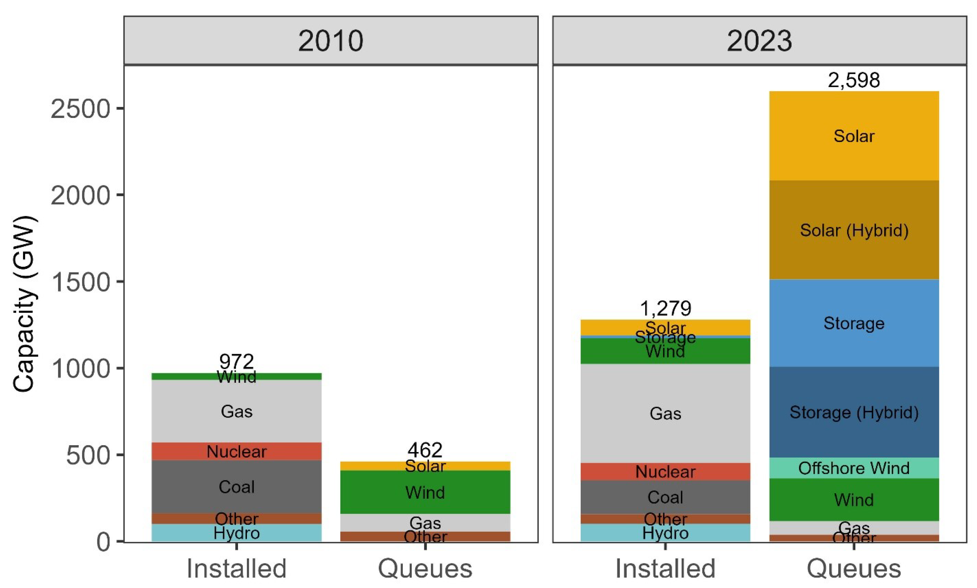
Figure 1. Installed generation capacity and queued interconnection requests in the United States in 2010 and 2023, by technology type. While total installed capacity increased modestly, the volume and composition of queued projects shifted dramatically, with solar, storage, and hybrid configurations dominating recent interconnection requests. Source: [2].
Energies 18 04832 g001
Figure 2. Process flow diagram for the proposed methodology. Red arrows represent repeated snapshot evaluation across scenario blocks. Green arrows represent optimal corrective actions per critical contingency. Magenta arrows represent repeated sampling from the same index. Blue arrows denote possible inclusion of forecast and planning data.
Energies 18 04832 g002
Figure 3. Comparison of two load sampling methods for the IEEE-14 bus system [35]. (Left) Uniform load scaling applied to all buses to simulate system-wide load levels at 80%, 100%, and 120% of the base case. (Right) Gaussian sampling of active power loads at each bus, introducing spatial diversity through independent normal distributions centered on nominal values with bus-specific variability.
Energies 18 04832 g003
Figure 4. Illustration of raw and distributional sampling methods using summer weekday CAISO load data. (Left) Full-day profiles are sampled directly from time series, with one day highlighted and representative load points and blocks annotated. (Middle) A multivariate Gaussian distribution is used to generate load samples based on empirical mean and covariance, showing a sampled profile and the 95% confidence interval (CI). (Right) Covariance matrix capturing hour-to-hour dependencies among summer weekday profiles.
Energies 18 04832 g004
Figure 5. Spring weekday profiles of solar (top) and wind (bottom) generation in 2019. (Left) Raw samples with one sampled day, point, and block highlighted. (Middle) Distributional sampling from empirical mean and covariance, including 95% confidence interval. (Right) Covariance matrix showing hourly dependencies.
Energies 18 04832 g005
Figure 6. Illustrative merit order diagram. Existing generators have varying marginal costs (e.g., 25–80 USD/MWh), while all candidate DERs are assigned a fictitious, equally high cost (e.g., 100 USD/MWh), ensuring they are only dispatched when required by physical constraints.
Energies 18 04832 g006
Figure 7. Comparison of case-based snapshots and time block scenarios. Each sampled base solution S i , j is linked to a set of critical contingency subproblems { S i , j c } ; for blocks, sequential timesteps are linked via their base solutions. Post-contingency states are not propagated forward in time, which limits branching and keeps the workflow tractable for large networks and longer horizons.
Energies 18 04832 g007
Figure 8. Illustration of Puerto Rico’s bulk power system (BPS), including transmission infrastructure and major generating facilities. Here, 115 kV lines are shown in red, and 230 kV lines are shown in blue. The six largest generating facilities (by capacity) are shown.
Energies 18 04832 g008
Figure 9. Boxplots of bus voltage magnitudes across all base and N-1 contingency scenarios and all retirement stages. Buses are sorted left to right by mean voltage. For each bus, boxes show the interquartile range across scenarios; whiskers indicate the non-outlier range; and points mark outliers. The bold red line marks the mean across scenarios. Nominal upper and lower voltage limits are shown to highlight violating outliers. Most scenarios are feasible; marginal excursions appear as isolated outliers.
Energies 18 04832 g009
Figure 10. Boxplots of line/transformer loading across all base and N-1 contingency scenarios and all retirement stages. Boxes show the interquartile range; whiskers indicate the non-outlier range; and points mark outliers. A faint horizontal line shows Rate A thermal limits for reference. Elements are sorted by their Rate A limit (descending) to make headroom visible. Across scenarios, flows remain within Rate A limits.
Energies 18 04832 g010
Figure 11. Boxplots of active power dispatch for each candidate DER site across all scenarios in the final retirement stage. The bold red line marks expected utilization (mean across scenarios); boxes show the interquartile range; and points indicate outliers. Sites are sorted by mean dispatch to highlight which DERs were most called upon and at what output. Since the candidate reserve cost structure was used, expected utilization can be interpreted as a deliverability indicator, highlighting deliverable power injections from preferential locations under network constraints.
Energies 18 04832 g011
Figure 12. Geospatial view of expected DER utilization (MW) across all scenarios in the final retirement stage, centered on node locations in the public BPS model. Marker size reflects higher expected MW dispatch; clusters indicate high utilization density. The analysis highlights Humacao as the highest-density region, followed by Vega Alta, with San Juan exhibiting many smaller sites, consistent with rooftop PV patterns. These insights indicate where solicitations (RFPs) may yield the most impact.
Energies 18 04832 g012
Figure 13. Mean reactive power contributions from candidate DERs (MVar) across all base and N-1 contingency scenarios in the final retirement stage. Marker size reflects higher mean reactive power dispatch. Clusters highlight locations most in need of voltage support as legacy units retire, aligning with large load centers and industrial zones. When reactive support coincides with active dispatch, hybrid PV–battery sites are promising resources (coordinated P/Q control); where reactive support occurs without active output, the results suggest stand-alone compensation (e.g., shunt capacitors or synchronous condensers).
Energies 18 04832 g013
Table 1. Scenario-based reliability of feasible operations under successive retirement stages. Confidence intervals are computed using a 95% confidence level (CI).
Retirement StageReliability95% CI WidthNum. of Scenarios
(Feasible/Total)
R10.9444±0.105817/18
R20.9444±0.105817/18
R30.8889±0.145216/18
All0.9306±0.058767/72
Disclaimer/Publisher’s Note: The statements, opinions and data contained in all publications are solely those of the individual author(s) and contributor(s) and not of MDPI and/or the editor(s). MDPI and/or the editor(s) disclaim responsibility for any injury to people or property resulting from any ideas, methods, instructions or products referred to in the content.