Machine Learning-Based Prediction of Heat Transfer and Hydration-Induced Temperature Rise in Mass Concrete

Abstract

The temperature rise in mass concrete structures, caused by the exothermic process of cement hydration and concurrent heat exchange with the environment, results in thermal gradients between the core and outer layers of the structure. These gradients generate tensile stresses that may exceed the early age tensile strength of concrete, leading to cracking. Therefore, reliable prediction of the temperature rise and associated thermal gradients is essential for assessing the risk of early age thermal cracking. Traditional methods for predicting temperature development rely on numerical simulations and simplified analytical approaches, which are often time-consuming and impractical for rapid engineering assessments. This paper proposes a machine learning-based (ML) approach to predict temperature rise and thermal gradients in mass concrete. The dataset was generated using the analytical CIRIA C766 method, enabling systematic selection and gradation of key factors, which is nearly impossible using measurements collected from full-scale structures and is essential for identifying an effective ML model. Three regression models, linear regression, decision tree, and XGBoost were trained and evaluated on simulated datasets that included concrete mix parameters and environmental conditions. Among these, the XGBoost model achieved the highest accuracy in predicting the maximum temperature rise and the temperature differential between the core and surface of the analysed element. The results confirm the suitability of ML models for reliable thermal response prediction. Furthermore, ML models can provide a usable alternative to conventional methods, offering both tools to thermal control strategies and insight into the influence of input factors on temperature in early age mass concrete.

1. Introduction

The hydration process in mass concrete is a complex phenomenon influenced by numerous interrelated factors. Among these, the heat generated during cement hydration plays a critical role in the early age behaviour of concrete. Excessive temperature rise can lead to thermal gradients and internal restraints, which in turn contribute to the development of thermal cracking, a significant durability concern in large-scale concrete structures. Early theoretical investigations into the heat of hydration date back to the 1930s, notably during the construction of the first dams. Since then, decades of research have focused on mitigating thermal cracking by optimising cement types, concrete mix designs, curing methods, and the use of chemical and mineral admixtures [1,2,3,4,5,6,7,8,9,10,11,12,13,14].

Contemporary research continues to highlight the importance of modelling heat and mass transfer in concrete, with an increasing number of studies over the past three years confirming the persistent relevance of this subject [15,16,17,18]. Foundational models for heat and moisture transport in porous materials were first proposed by Luikov, Harmathy, and De Vries [15,19]. Today, a wide range of mathematical and numerical models are available, varying in terms of physical assumptions and computational complexity. Advanced models for concrete specifically incorporate its porous, multi-phase character and the interplay of physicochemical phenomena [12,20,21]. However, many engineering applications, especially those involving early age massive concrete structural members, still rely on simplified formulations that neglect thermodiffusion cross-effects [22,23,24,25]. While more comprehensive formulations derived from the laws of irreversible thermodynamics do exist [16,20], their practical application is limited by complexity and computational demands. Consequently, simplified 1D or 2D analyses are often used, omitting the spatial variability of temperature and moisture fields, especially in irregularly shaped elements such as bridge abutments, nuclear containment walls, or lock chambers.

Heat and moisture transport in concrete generally follow Fourier’s law and Fick’s second law, respectively. Yet, the hydration phase presents unique modelling challenges. Initially a heterogeneous mixture of solids and liquids, concrete undergoes significant structural transformation as hydration progresses, complicating the modelling of its thermal response. Two main modelling strategies address this: the multi-phase and phenomenological approaches [12].

The multi-phase approach seeks to represent the material’s heterogeneous nature through separate constitutive equations for the solid, liquid, and gaseous phases. These are then averaged to describe the behaviour of the concrete as a whole. Although this method can offer detailed insights, it involves numerous input parameters and is computationally intensive. Research by Gawin et al. [20] and others [26,27] has advanced multi-phase modelling significantly. Nevertheless, due to computational limitations, even these sophisticated models often reduce the analysis to one-dimensional cases, limiting the evaluation of spatial heat and humidity distributions in massive elements.

In contrast, the phenomenological approach treats concrete as a continuous medium and provides a macroscopic description of heat and mass transport phenomena. This strategy is more popular in engineering applications and is supported by numerous studies. A detailed review of these models and their capabilities is presented in [15]. While this method is less computationally demanding, it still requires a deep understanding of the evolving thermal properties of concrete and access to advanced modelling tools to deliver reliable predictions.

As mentioned before, the challenges posed by early age thermal effects in concrete became evident during the 19th and 20th centuries, particularly with the construction of massive concrete dams. Landmark projects such as the Hoover Dam (1936) and the Grand Coulee Dam (1942) in the United States exposed the critical issue of excessive heat generated by cement hydration [1,2]. Today, similar problems persist in modern infrastructure, particularly in large-scale structural elements such as foundation blocks, bridge abutment walls, reactor containments, water tanks, and retaining walls [17,28,29]. These elements, characterised by thick cross-sections, are collectively referred to as mass concrete due to their susceptibility to significant temperature rises during hydration.

The heat generated within these elements can reach up to 100 °C, giving rise to two major concerns. First, high internal temperatures must be limited, typically to 65–70 °C, to avoid delayed ettringite formation (DEF), which poses long-term risks to concrete durability. Second, non-uniform temperature distribution creates thermal gradients, as the core of the structure heats up and cools more slowly than the exterior. This mismatch in expansion and contraction causes internal restraint and tensile stresses, resulting in thermal cracking. In the case of external restraints, which are typical in building structures, tensile stresses due to this restraint arise during the cooling phase, as the maximum temperature reached in the element gradually decreases to ambient temperature. The formation of thermal cracks not only weakens the mechanical performance of the structure but also compromises watertightness, which is especially critical in hydraulic and containment structures. To mitigate this risk, construction guidelines often impose maximum allowable differences in temperature, both between the core and surface (commonly 15–20 °C) and between the peak and stabilised temperatures, to ensure concrete strains remain within acceptable limits [2,3]. Therefore, accurately predicting temperature rise in concrete during this critical early period is essential for achieving durable, crack-resistant structures. Numerous research efforts and real-world case studies have emphasised the importance of this issue and the limitations of existing modelling tools.

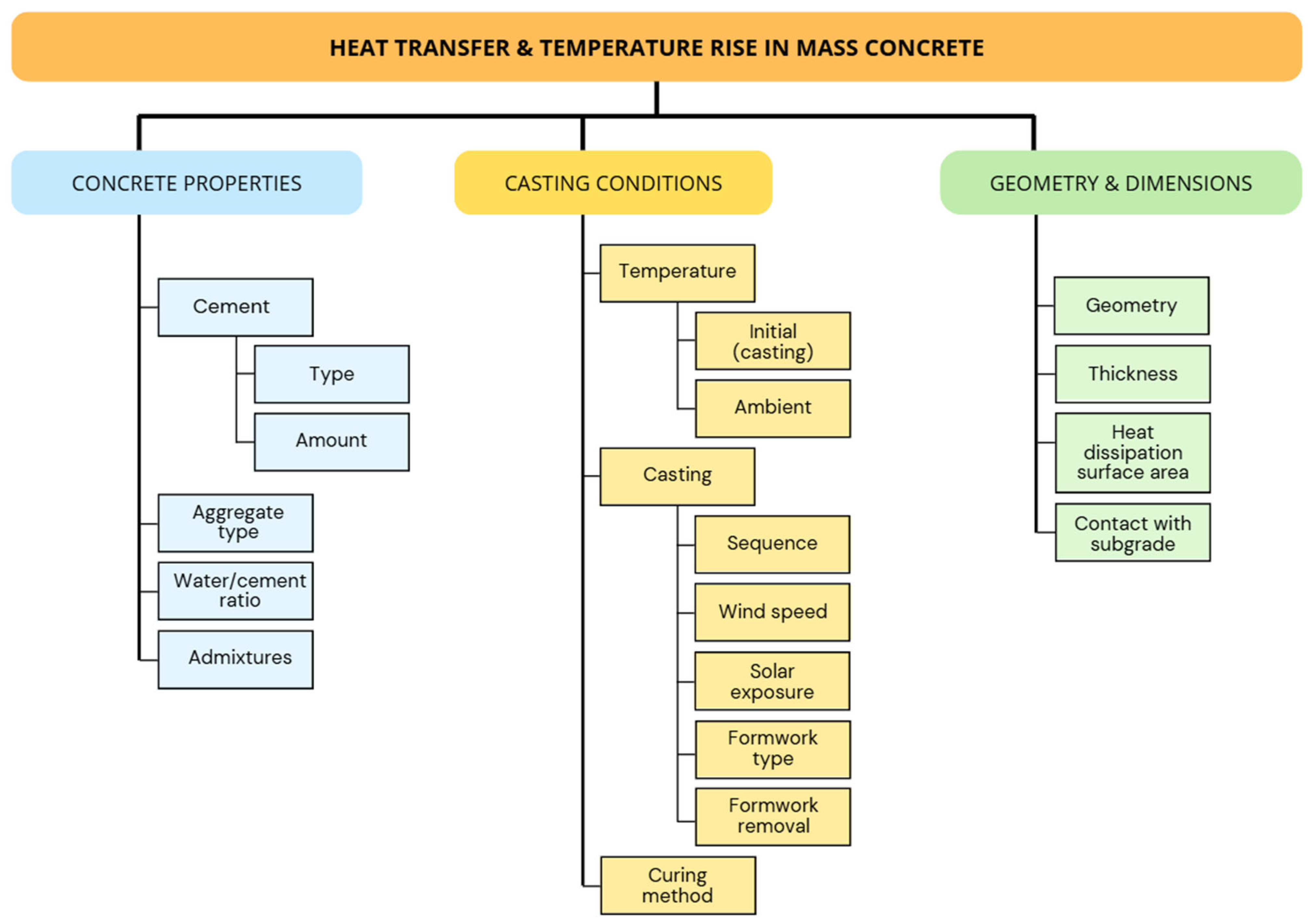
There is a large number of interdependent factors that influence temperature development during both the hydration process and the transfer of heat to the environment. These factors are complex, often nonlinear, and highly sensitive to variations in both material characteristics and external conditions. For clarity, they can be grouped into three main categories (Figure 1).

The first group encompasses the properties of the concrete mix, including the type and quantity of cement, the use of mineral and chemical admixtures, the water-to-cement ratio, and particularly the type of aggregate. These factors primarily affect the amount of heat generated during hydration, but they also influence heat transfer characteristics—particularly through the aggregate, which plays a key role in determining the thermal conductivity of the concrete.

The second group includes casting and curing conditions, such as the initial temperature of the mix at placement, ambient temperature during construction, the casting sequence, duration and segmentation, the thermal properties of the formwork, and the type of curing or protection applied to exposed surfaces. Environmental factors like solar radiation and wind speed also fall into this category, as they significantly affect heat exchange between the concrete and its surroundings.

The third group involves geometric and boundary conditions, including the dimensions and thickness of the structural element, the nature of contact with the subgrade or adjacent materials, and the available surface area for heat dissipation. These aspects strongly influence how heat is retained or lost over time. All of these factors interact dynamically throughout the hydration and hardening process. Moreover, the kinetics of cement hydration, which themselves depend on the evolving temperature field within the concrete, add a layer of complexity. As a result, the accurate prediction of thermal behaviour in mass concrete requires not only detailed thermal modelling but also calibration of model parameters using experimental data and validation through real-time temperature monitoring.

Given the complexity of interacting factors influencing heat transfer in mass concrete, as well as the limitations of current analytical and numerical methods—many of which are either oversimplified or computationally prohibitive—there is a growing demand for novel, efficient, and reliable predictive approaches. Traditional simulations often require the use of advanced computational software, substantial processing power, and detailed description and calibration of material parameters, which significantly limit their practicality in real-time engineering applications [15,22,30]. In this context, the use of machine learning (ML) offers a promising alternative [31,32,33,34]. By learning directly from data, ML models can capture complex nonlinear relationships among multiple variables governing temperature rise, temperature distribution, and thermal gradients. This is particularly valuable given that temperature development in mass concrete is inherently nonlinear, nonstationary, and affected by numerous interacting factors. While the problem can, in principle, be solved using the three-dimensional Fourier heat conduction equation with appropriate boundary conditions, such solutions require advanced numerical modelling and are computationally demanding. On the other hand, simplified physical estimations are feasible only under idealised adiabatic conditions, which neglect environmental heat exchange and therefore fail to represent real structures. These limitations highlight the need for alternative approaches that can provide sufficiently accurate predictions while accounting for diverse influencing technological and materials factors. ML methods may address this gap by offering a systematic framework for predicting early age thermal behaviour in mass concrete structures. Once an appropriate model is trained and validated on an expanded database, it could serve as a practical tool for engineers to estimate temperature development across a broad range of input parameters. Moreover, beyond prediction, ML can also help quantify the relative importance of technological and material factors, thereby supporting better-informed design decisions and more effective thermal control strategies.

It should be mentioned that in recent years, AI has introduced new perspectives and transformative approaches in the study of cementitious materials. Innovative numerical procedures and modelling techniques have been proposed, enabling the analysis of temperature and stress fields in mass concrete based on existing finite element simulations combined with the development of data-driven methods [35]. For example, during the construction of a large-span cable-stayed bridge in China, Support Vector Regression (SVR) was successfully used to predict the heat of hydration in pile caps based on monitoring data. The model achieved high accuracy in forecasting temperature 2–3 days in advance and outperformed traditional BP neural networks [36]. Similarly, deep learning (DL) techniques—such as Artificial Neural Networks (ANN), Recurrent Neural Networks (RNN), and Bidirectional Deep RNNs (BD-RNN)—have shown promise in predicting temperature rise in concrete with complex mix compositions. Enhanced with segmentation methods, optimisation algorithms, and cross-validation, these models achieved reliable results even when trained on relatively small datasets [37]. In addition to thermal prediction, machine learning models are also used to address complex engineering problems, offering improved accuracy and efficiency [34,36,37,38,39,40,41,42,43,44].

Particularly useful and worthy of attention may be regression machine learning models, designed to predict continuous numerical values based on input data. Regression machine learning models are a class of algorithms designed to predict continuous numerical values based on input data. Unlike classification models, which assign data points to predefined categories, regression models learn the underlying relationship between input features and a continuous target variable. In the context of building materials engineering, such models can be especially valuable for forecasting key parameters in early age concrete behaviour. For example, predicting the maximum temperature inside mass concrete elements, estimating the rate of heat release from cement hydration, or modelling the development of temperature gradients during curing. Commonly used regression algorithms include linear regression, which assumes a straightforward linear relationship between inputs and outputs; decision trees and ensemble methods like Random Forest, which can capture complex, nonlinear patterns; Support Vector Regression (SVR), which is well-suited for high-dimensional data; and neural networks, which are capable of modelling intricate nonlinear dependencies due to their layered architecture [33,36]. Additionally, ensemble-based approaches such as gradient boosting combine multiple weak learners to create a more accurate and robust predictive model. Once trained on relevant datasets, these models can deliver rapid and precise predictions, reducing reliance on traditional, time-consuming physical simulations. Their ability to account for multiple interacting variables and nonlinear relationships makes them a powerful tool in modelling the thermal and durability performance of mass concrete structures.

Despite promising results, ML applications in the context of heat transfer prediction in mass concrete are still not widespread. Therefore, this paper proposes a machine learning-based framework for predicting temperature rise and thermal gradients induced by cement hydration and heat transfer to the environment. It should be mentioned that the proposed ML models are designed to predict the maximum temperature and temperature gradients in mass concrete. The thermal cracking risk, the most relevant aspect from a practical perspective, is not directly predicted; however, it can be evaluated based on the predicted peak temperature, the subsequent cooling to ambient conditions, and the magnitude of the thermal gradient. In practice, given the limiting tensile strain capacity of concrete, it is generally assumed that the temperature gradient should not exceed approximately 15–20 °C. Thermal gradients also provide the basis for stress calculations. Therefore, temperature prediction consistently serves as the foundation for assessing the potential risk of thermal cracking.

Three regression models, linear regression, decision tree, and XGBoost were trained and evaluated on simulated datasets that included concrete mix parameters and environmental conditions. The method is shown through a case study of a massive reinforced concrete wall, a structural element commonly used in bridge abutments, nuclear enclosures, lock walls, tanks, and retaining structures. These components are particularly vulnerable to early age cracking due to hydration heat accumulation, which may reduce their serviceability and durability.

The remainder of this paper is structured as follows. In the Data and Methods section, we describe the input data, the generation of simulation datasets, and the applied machine learning algorithms. This section also outlines the data preprocessing steps and training strategy. The Results section presents the model’s predictive performance and compares it with traditional simulation approaches. Finally, conclusions are drawn regarding the effectiveness, limitations, and potential of ML-based modelling for early age thermal behaviour in mass concrete temperatures.

2. Data and Methods

2.1. Data Collection

The development of temperature during concrete curing was estimated using the iterative method outlined in CIRIA C766 [3,29], which proposed a useful approach for predicting temperature rise and thermal gradients based on adiabatic temperature data. This method is based on heat diffusion theory and applied through spreadsheet-based calculations. Previous studies have demonstrated good agreement between this prediction method, full 3D finite element models as well as experimental measurements [29]. In detail, the method assumes that the temperature at a given cell and time step is calculated as the average of the temperatures in the surrounding cells from the previous time step, with an additional increment corresponding to the adiabatic temperature increase during that time interval. The procedure follows the formula:

$$T_{t,j}=0.5\left(T_{t-\mathsf{\Delta }t,j-1} + T_{t-\mathsf{\Delta }t,j+1}\right)+∆T_{ad}$$

where

$T_{t,j}$—the temperature within a cell at a particular time increment $t$, in the cell $j$,

$T_{t-\mathsf{\Delta }t,j-1}$, $T_{t-\mathsf{\Delta }t,j+1}$—the temperature within the previous time increment $t-\mathsf{\Delta }t$ in the adjacent cells $j-1$, $j+1$,

$∆T_{ad}$—the adiabatic temperature rise within the time increment $t$.

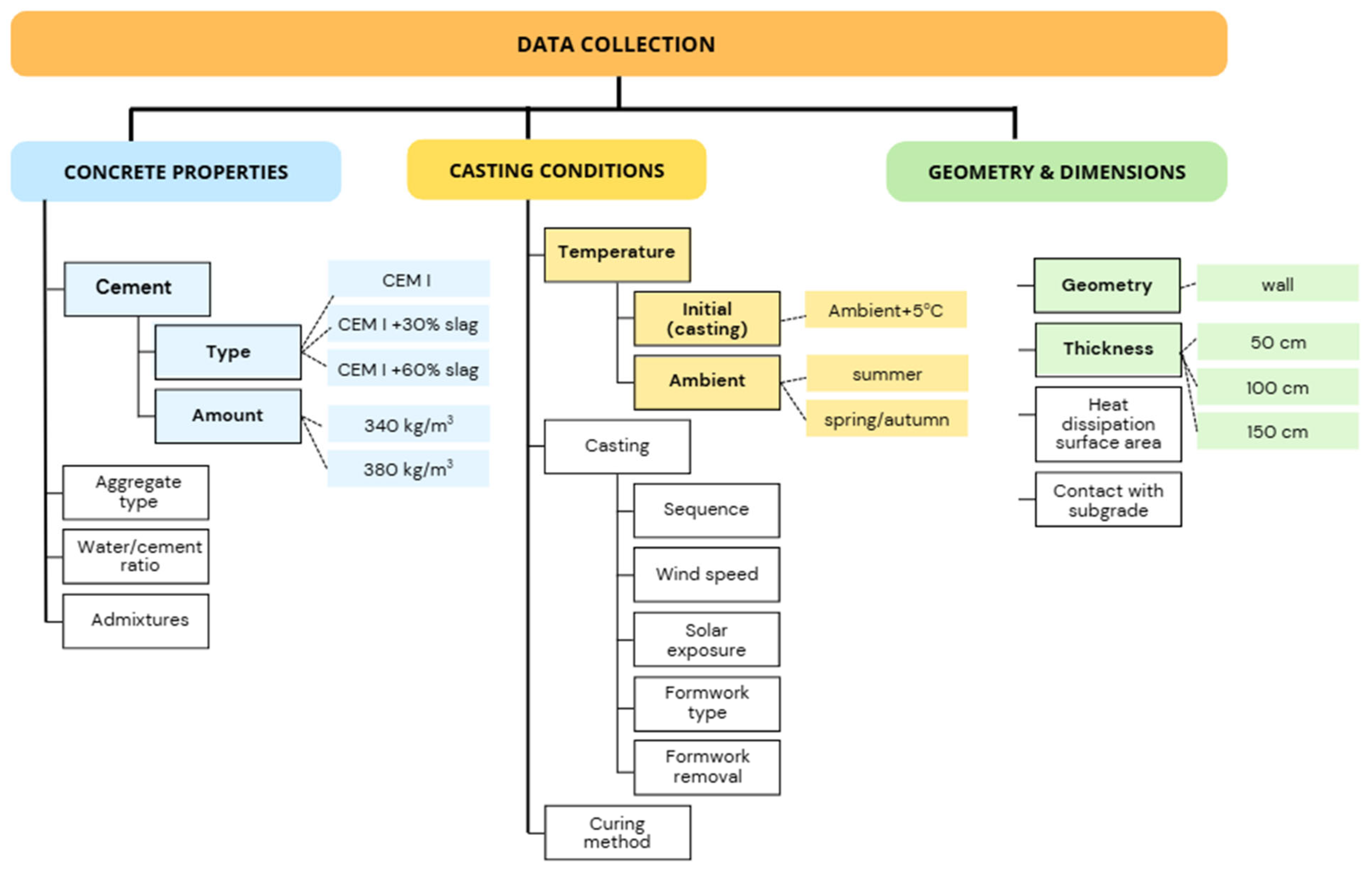
It should be emphasised that the dataset was generated entirely using the CIRIA C766 analytical method and does not include experimental or field monitoring data. This approach was chosen to enable a systematic and controlled variation in key factors, which is extremely difficult to achieve in real massive concrete structures due to the large number of variable conditions. Although

Table 1. Data collections set.

Wall Thickness, cm	Concrete Class	Cement Type	Total Binder, kg/m3	Environmental Conditions	Initial Temperature, °C	Ambient Temperature, °C	Tmax, °C	ΔT Core_Surface, °C
50	C30/37	CEM I	340	spring/autumn	15	10	40	5.6
50	C30/37	CEM I	340	summer	30	25	63.7	7.3
50	C30/37	CEM I + 30% slag	340	spring/autumn	15	10	33.3	4.4
50	C30/37	CEM I + 30% slag	340	summer	30	25	58	6.2
50	C30/37	CEM I + 60% slag	340	spring/autumn	15	10	27.1	3.2
50	C30/37	CEM I + 60% slag	340	summer	30	25	50.9	4.9
100	C30/37	CEM I	340	spring/autumn	15	10	51.4	13
100	C30/37	CEM I	340	summer	30	25	72.3	14.7
100	C30/37	CEM I + 30% slag	340	spring/autumn	15	10	44	10.7
100	C30/37	CEM I + 30% slag	340	summer	30	25	67.1	13.1
100	C30/37	CEM I + 60% slag	340	spring/autumn	15	10	35.8	8.1
100	C30/37	CEM I + 60% slag	340	summer	30	25	59.2	10.7
150	C30/37	CEM I	340	spring/autumn	15	10	57.8	19.2
150	C30/37	CEM I	340	summer	30	25	76.1	20.1
150	C30/37	CEM I + 30% slag	340	spring/autumn	15	10	50.8	16.5
150	C30/37	CEM I + 30% slag	340	summer	30	25	71.6	18.5
150	C30/37	CEM I + 60% slag	340	spring/autumn	15	10	41.8	13
150	C30/37	CEM I + 60% slag	340	summer	30	25	63.8	15.5
50	C35/45	CEM I	380	spring/autumn	15	10	43.1	6.2
50	C35/45	CEM I	380	summer	30	25	68	8.1
50	C35/45	CEM I + 30% slag	380	spring/autumn	15	10	35.8	4.9
50	C35/45	CEM I + 30% slag	380	summer	30	25	61.6	6.9
50	C35/45	CEM I + 60% slag	380	spring/autumn	15	10	28.9	3.6
50	C35/45	CEM I + 60% slag	380	summer	30	25	53.7	5.4
100	C35/45	CEM I	380	spring/autumn	15	10	55.8	14.4
100	C35/45	CEM I	380	summer	30	25	77.6	16.3
100	C35/45	CEM I + 30% slag	380	spring/autumn	15	10	47.5	11.8
100	C35/45	CEM I + 30% slag	380	summer	30	25	71.7	14.6
100	C35/45	CEM I + 60% slag	380	spring/autumn	15	10	38.4	9
100	C35/45	CEM I + 60% slag	380	summer	30	25	63	11.9
150	C35/45	CEM I	380	spring/autumn	15	10	62.9	21.3
150	C35/45	CEM I	380	summer	30	25	81.7	22.3
150	C35/45	CEM I + 30% slag	380	spring/autumn	15	10	55.1	18.3
150	C35/45	CEM I + 30% slag	380	summer	30	25	76.7	20.5
150	C35/45	CEM I + 60% slag	380	spring/autumn	15	10	45.1	14.3
150	C35/45	CEM I + 60% slag	380	summer	30	25	68	17.2

presents only a limited set of parameters, these were selected as the most influential for early age thermal behaviour. Other factors, such as curing methods, formwork removal time, and wind speed, were kept constant to ensure a manageable dataset size and effective training and evaluation of the ML models. It should also be noted that obtaining full experimental data in this context is highly challenging, as it would require not only temperature measurements in massive concrete elements but also, among others, measurements of cement hydration heat, thermal properties of concrete, ambient temperature, and wind speed. As mentioned in the Introduction, the application of ML in assessing the temperature development of hardening concrete is still not widespread; therefore, as a first step, this analytical approach was considered more suitable to evaluate the potential of ML models. We acknowledge that this limits the diversity of the dataset, and future work incorporating experimental or field data will be essential to improve the representativeness and generalisation of the models.

The factors considered in the analysis are highlighted in Figure 2, encompassing all key parameters that influence heat transfer and temperature rise in mass concrete. The structural element analysed was a concrete wall, intended to represent walls of varying thickness. It should be noted that in such elements, thickness is the main factor affecting temperature development during hydration; therefore, other dimensions were not specified in the analysis. It should be noted that the binder contents of 340 kg/m³ and 380 kg/m³ were selected based on the guidelines [3] and correspond to the target concrete classes C30/37 and C35/45, respectively.

The remaining input parameters, kept constant across all cases, were as follows: gravel aggregate and quartz sand, no chemical admixtures, wind speed of 5 m/s, and 18 mm plywood formwork. Variables such as formwork removal time, segmented concreting, and the use of temperature-reducing methods were not considered in the analysis. Heat transfer was assumed to occur solely through the side formwork surfaces.

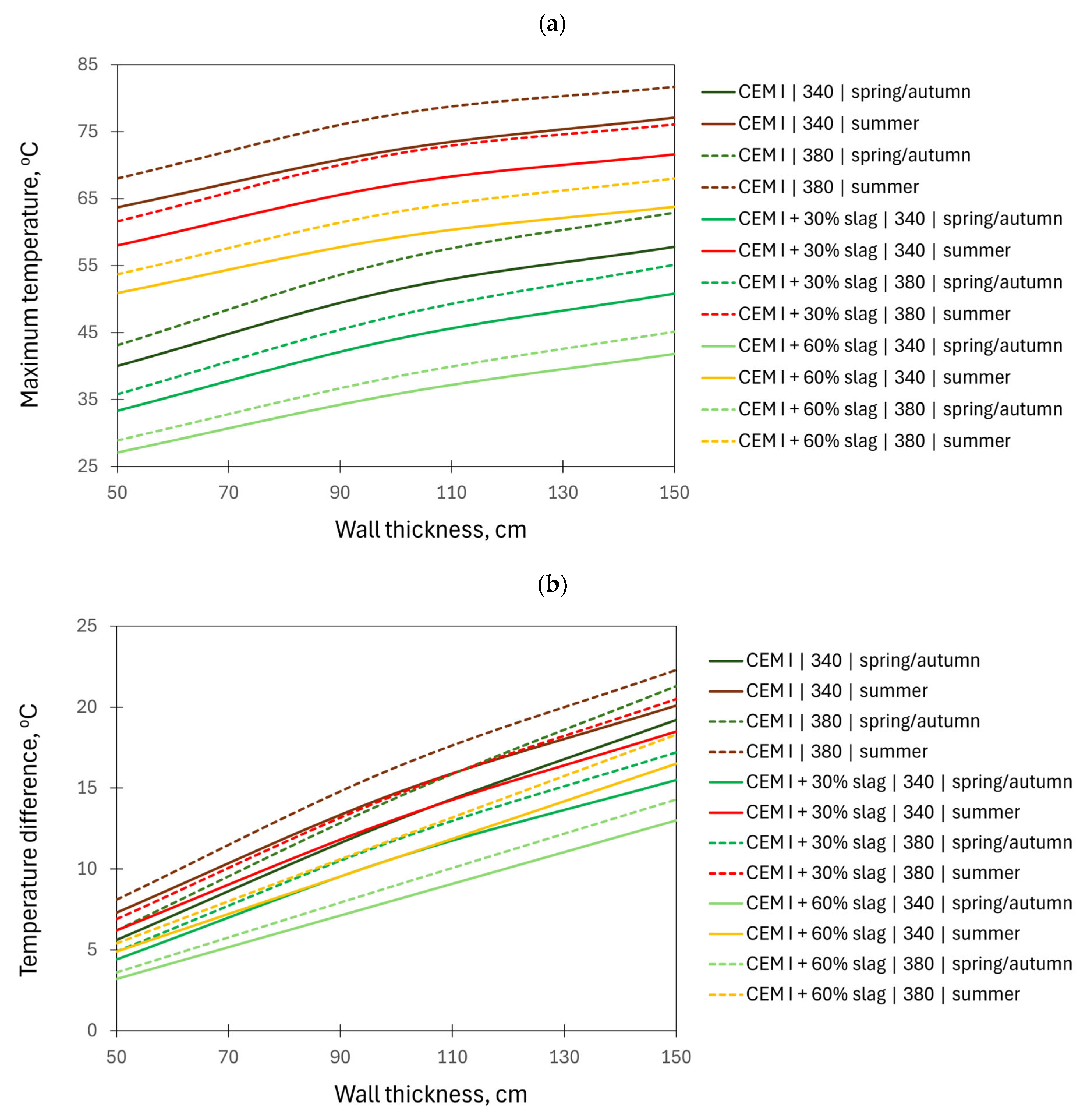
Figure 3 and Table 1 present two key temperature values obtained from the calculations for the wall: the maximum internal temperature (Figure 3a) and the temperature difference between the wall’s interior and exterior surfaces (Figure 3b) across all analysed cases.

2.2. Data Distribution Analysis

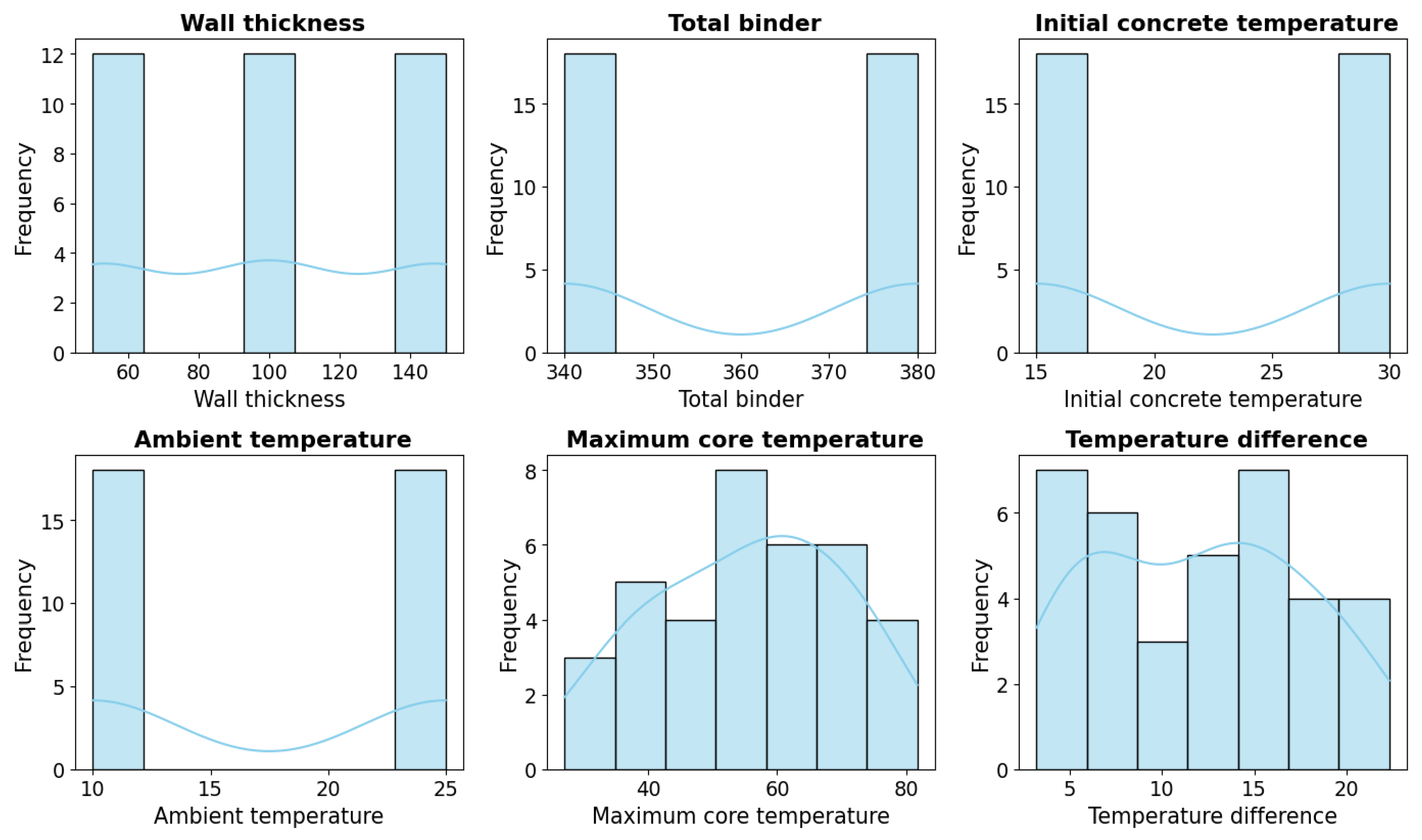
The data distribution was evaluated using both descriptive statistics (

Table 2. Descriptive statistics of numerical variables.

Variable	Mean	Std	Min	25%	50%	75%	Max
Wall thickness	100.00	41.4039	50.00	50.00	100.0	150.0	150.00
Total binder	360.00	20.2837	340.00	340.00	360.0	380.0	380.00
Initial concrete temperature	22.50	7.6064	15.00	15.00	22.50	30.00	30.00
Ambient temperature	17.50	7.6064	10.00	10.00	17.50	25.00	25.00
Maximum core temperature	55.5361	14.7690	27.10	43.775	56.80	67.325	81.70
Temperature difference	11.9917	5.6566	3.20	6.725	12.45	16.350	22.30

) and histograms (Figure 4), which confirmed the absence of strong skewness or extreme outliers. The variables exhibited relatively narrow ranges and showed no evidence of outliers. For instance, Wall thickness and Total binder varied in discrete steps (50–150 cm and 340–380 kg/m³, respectively), while temperature-related variables (Temp initial and Temp ambient) ranged from 15 to 30 °C and 10–25 °C. In contrast, the output variables were more variable: Tmax ranged from 27.1 to 81.7 °C (mean 55.5 °C), and ΔT core_surface ranged from 3.2 to 22.3 °C (mean 12.0 °C). Although the distributions did not strictly conform to normality, no substantial skewness or outliers were observed. Accordingly, the dataset was deemed suitable for machine learning modelling without the need for further transformations.

In the analyses, various strategies for preprocessing input data were tested, including normalisation of numerical features and the use of regularised linear models. Normalisation was specifically evaluated in the context of linear regression, as this type of model can be sensitive to differences in feature scales. However, in the present dataset, the numerical features fell within comparable ranges (approximately 10–400), which did not introduce substantial disparities between variables. As a result, normalisation did not lead to any meaningful improvement in model performance and, in some cases, even caused a slight deterioration in results. Similarly, the application of regularisation had no notable effect on error metrics. Therefore, the final analyses employed classical linear regression without additional scaling. It is also worth noting that for tree-based models (Decision Tree, XGBoost), normalisation is not required, since these algorithms rely on threshold-based splits rather than regression coefficients. Consequently, scaling has no impact on their performance. In summary, scaling was evaluated but ultimately omitted in the final analyses, as it did not improve predictive performance in linear regression and was irrelevant for tree-based models.

2.3. Methods

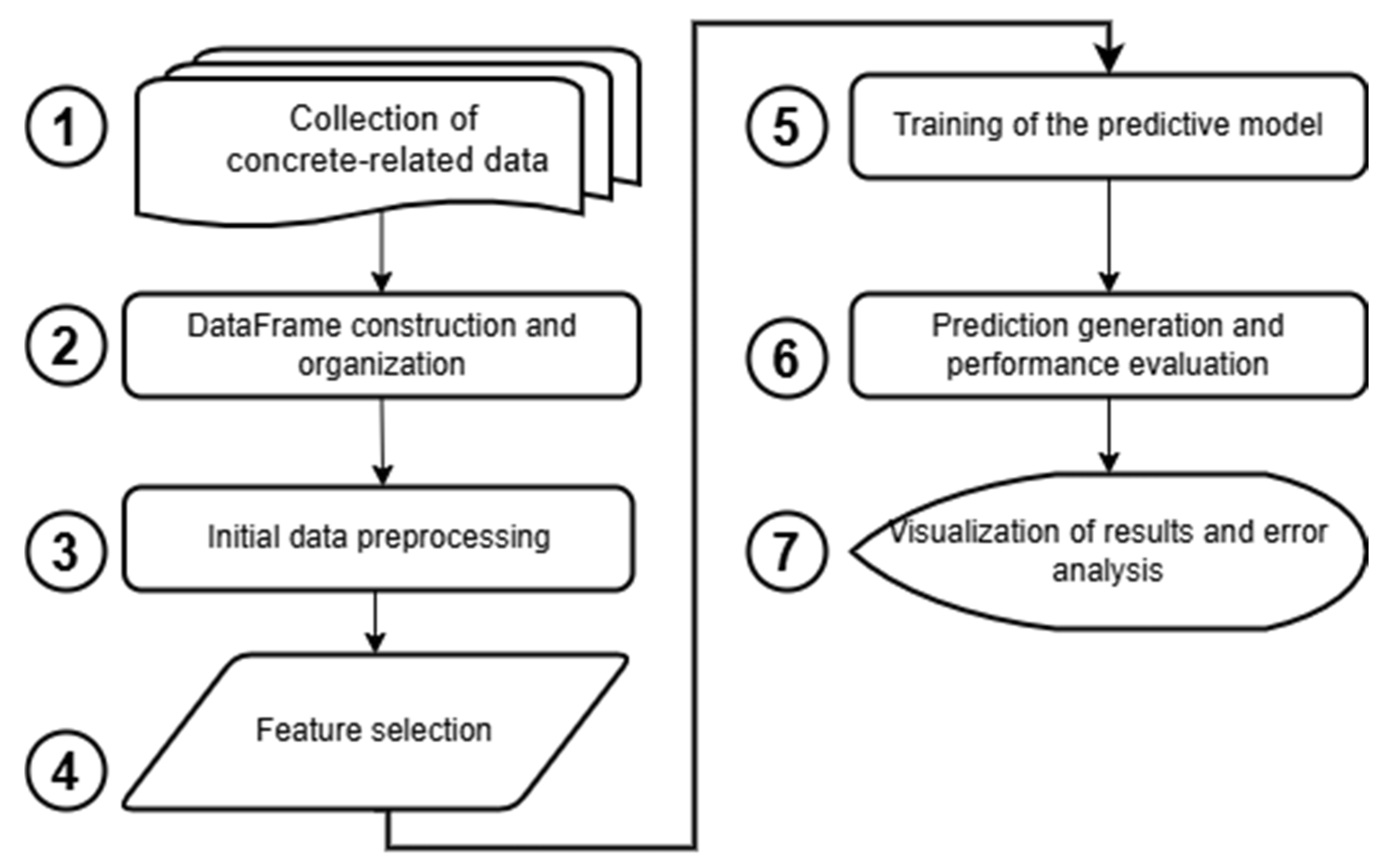
In the first step (Figure 5, Step 1), a dataset of experimental results related to the properties of mass concrete walls, as described in the previous section, was compiled. The data, visualised in Figure 3, were organised into columns representing the following parameters: wall thickness, concrete class, cement type, slag content (Slag), total binder content, initial mix temperature (Temp initial), constant ambient temperature (Temp ambient), maximum temperature during hydration (Tmax), and the temperature difference between the core and the surface of the element (ΔT core_surface).

It should be outlined that the variables with potentially low correlation were retained deliberately to allow the ML models to assess their potential combined influence and to avoid excluding factors that might have nonlinear, or interaction effects not captured by simple correlation analysis. Moreover, such low-correlation variables do occur in real massive concrete structures, which is why they were not omitted. Regarding validation, the dataset was generated using the analytical CIRIA C766 method, which allowed systematic variation in key factors but limited the availability of an independent or external dataset. Therefore, both LOOCV and 5-fold cross-validation were applied to maximise the effective use of the generated dataset and to provide a robust internal assessment of model performance, acknowledging that external validation would be desirable in future studies as real-field data becomes available.

The data were structured into a DataFrame (Figure 5, Step 2) using the Python version 3.12.6 pandas library, which facilitated further processing and analysis. During the preprocessing stage (Figure 5, Step 3), categorical variables were converted into a numerical format through encoding, making them compatible with machine learning algorithms.

Based on feature-importance analysis and the specific characteristics of the problem (Figure 5, Step 4), a subset of relevant input variables was identified and is presented in

Table 3. List of Input variables (Features) used in the study.

Variable	Description
Wall thickness (cm)	Thickness of the concrete wall
Concrete class	Strength class of the concrete mix
Slag content (%)	% of ground granulated blast-furnace slag
Total binder (kg/m3)	Total amount of binder materials
Environmental conditions	Seasonal environmental conditions
Initial concrete temperature (°C)	Temperature of fresh concrete at casting
Ambient temperature (°C)	Ambient temperature during hydration

. The machine learning models were then configured to predict two target outputs: the maximum temperature (Tmax) and the temperature difference between the concrete core and surface (ΔT core_surface), as summarised in

Table 4. List of Output variables (Targets) used in the Study.

Variable	Description
Maximum core temperature (Tmax, °C)	Peak temperature in the core of the wall
Temperature difference (ΔT core_surface, °C)	Temperature difference between the core and the wall surface

.

To predict the thermal response of concrete, three regression machine learning models were employed (Figure 5, Step 5): linear regression—a basic statistical model that estimates the target value as a linear combination of input features; decision tree—an algorithm that constructs a tree-like structure by recursively partitioning the data based on feature values; and XGBoost—a powerful gradient boosting technique that builds an ensemble of models by iteratively correcting the errors of previous predictions.

Linear regression analysis is a widely used statistical technique that models the relationship between variables and predicts the value of one variable based on another. The variable to be predicted is known as the dependent variable, while the variable used for prediction is the independent variable. Simple linear regression examines the relationship between a continuous outcome variable and a continuous covariate. This relationship is assumed to be linear and is typically represented by the equation in which x is the covariate and y the outcome: y = β₀ + β₁x. Here, β₀ is the intercept of the straight line and the y-axis, and β₁ is the slope of the line. Since β₀ corresponds to the value of y when x is zero, it often holds limited practical significance and is rarely the focus of analysis. When the model includes multiple covariates, it is referred to as multiple linear regression. Like simple linear regression, it uses the least squares method to estimate regression coefficients, though the calculations are more complex. Importantly, multiple linear regression is not limited to continuous variables; binary and categorical variables can also be incorporated into the model [31,32].

Decision trees are some of the most extensively studied and widely used tools in machine learning and data science. They are applied in various tasks, including classification, regression, and feature selection. The idea is to create a tree-like structure, where each node represents a decision or a split on a specific attribute. Algorithm recursively partitions data into subsets based on attribute values until a predefined stopping condition is met and selects the best attribute for each split using criteria like information gain and gain ratio. One of the key advantages of decision trees is their interpretability. The resulting model is easy to visualise and understand, which is particularly important in fields where transparency is crucial. Moreover, decision trees can handle both categorical and numerical data directly, avoiding the need for extensive preprocessing such as converting categorical variables into numerical formats. This versatility makes them efficient and effective in a broad range of applications [33].

XGBoost (Extreme Gradient Boosting) is a highly efficient machine learning algorithm based on the implementation of gradient-boosted decision trees. It is often used for supervised learning tasks, especially in regression and classification problems. XGBoost combines weak learners, decision trees, in sequence, where each new learner is trained to correct the errors of the previous ones. Like other supervised learning methods, for example, neural networks, XGBoost aims to minimise a loss function such as mean squared error for regression. Unlike neural networks that use backpropagation, XGBoost fits each tree to the negative gradient of the loss function relative to the model’s current predictions. Despite its strengths, XGBoost’s performance still depends on the quality and quantity of data. Another limitation is that the model’s tree-based structure does not yield a simple mathematical equation, which can limit interpretability. Additionally, its effectiveness can decrease when facing highly imbalanced datasets or when the relationship between variables is nonlinear and highly complex [34,45].

The training process was carried out using Leave-One-Out Cross-Validation (LOOCV), which provides a robust estimate of each model’s generalisation performance by evaluating it on all possible single-instance test sets.

For each iteration, the following performance metrics were recorded separately for both target variables: Mean Absolute Error (MAE) (Equation (1)), Mean Squared Error (MSE) (Equation (2)), Mean Absolute Percentage Error (MAPE) (Equation (3)), and the coefficient of determination (R²) (Equation (4)).

$$MAE:{\displaystyle \frac{1}{n}}\sum _{i=1}^n\left|y_i-\widehat{y_i}\right|$$

(1)

$$MSE:{\displaystyle \frac{1}{n}}\sum _{i=1}^n{\left(y_i-\widehat{y_i}\right)}^2$$

(2)

$$MAPE:{\displaystyle \frac{100\%}{n}}\sum _{i=1}^n\left|{\displaystyle \frac{y_i-\widehat{y_i}}{y_i}}\right|$$

(3)

$$R^2:1-{\displaystyle \frac{{\sum }_{i=1}^n{\left(y_i-\widehat{y_i}\right)}^2}{{\sum }_{i=1}^n{\left(y_i-\overline{y}\right)}^2}}$$

(4)

where

$y_i$—actual observed values;

$\widehat{y_i}$—predicted values;

$\overline{y}$—mean of actual values;

$n$—number of observations.

As a further evaluation step (Figure 5, Step 6), 5-fold cross-validation (5-fold CV) was performed for each model, with a focus on analysing the coefficient of determination (R²). In addition, a correlation analysis between input and target variables was conducted and presented in the form of a correlation matrix.

For each model (Figure 5, Step 7), the Permutation Importance method was used to assess the significance of individual features, enabling interpretation of their influence on the model’s predictions. To support this analysis, plots comparing actual and predicted values were generated, along with histograms of residuals (prediction errors). These visualisations helped identify potential areas where the models tended to underestimate or overestimate the predicted values, offering further insight into model performance and reliability.

3. Results

3.1. Model Performance Using Leave-One-Out Cross-Validation

To evaluate the accuracy of the predictive models, Leave-One-Out Cross-Validation (LOOCV) was used, as it provides reliable and stable results, particularly when working with a limited dataset. The evaluation outcomes are summarised in

Table 5. Comparison of regression model performance based on Leave-One-Out Cross-Validation.

Model	Target Variable	R2	MAE	MSE	MAPE (%)
Linear Regression	Tmax	0.983	1.573	3.511	3.013
Linear Regression	ΔT core_surface	0.975	0.726	0.770	8.321
Decision Tree	Tmax	0.925	3.856	15.892	6.994
Decision Tree	ΔT core_surface	0.944	1.206	1.728	10.265
XGBoost	Tmax	0.997	0.652	0.717	1.261
XGBoost	ΔT core_surface	0.998	0.176	0.048	1.948

, presented separately for each target variable: Tmax and ΔT core_surface.

Analysis of the results indicates that the XGBoost model delivered the best overall predictive performance, achieving the highest coefficient of determination (R²) values: 0.997 for Tmax and 0.998 for ΔT core_surface. Additionally, it recorded the lowest values of MAE, MSE, and MAPE, confirming its high level of accuracy and robustness. The linear regression model also performed well, with R² values of 0.983 for Tmax and 0.975 for ΔT core_surface, although its absolute errors were slightly higher compared to XGBoost.

The decision tree model, while still showing relatively high R² values (above 0.92 for both target variables), exhibited substantially larger prediction errors. This suggests a lower generalisation capability in this particular application, possibly due to overfitting or limited complexity in capturing the underlying relationships within the data.

3.2. Evaluation Using 5-Fold Cross-Validation

To further evaluate the generalizability of the models, five-fold cross-validation was conducted. For each model, the mean coefficient of determination (R²) and its standard deviation were calculated, enabling an assessment of the models’ predictive stability with respect to different training and test data splits.

As shown in

Table 6. Average R² and standard deviation of regression models based on 5-fold cross-validation.

Model	Mean R2	Standard Deviation
Linear Regression	0.9661	0.0105
Decision Tree	0.8985	0.0569
XGBoost	0.9665	0.0358

, the XGBoost model achieved the highest mean R² value of 0.9665, along with a moderate standard deviation of 0.0358, indicating both high predictive accuracy and good generalisation capability. The linear regression model yielded a slightly lower mean R² of 0.9661, but with the lowest standard deviation (0.0105), suggesting excellent consistency and stability across cross-validation iterations.

In contrast, the decision tree model recorded the lowest mean R² value (0.8985) and the highest standard deviation (0.0569), reflecting greater variability in results and reduced prediction stability compared to the other models.

3.3. Correlation Between Input and Target Variables

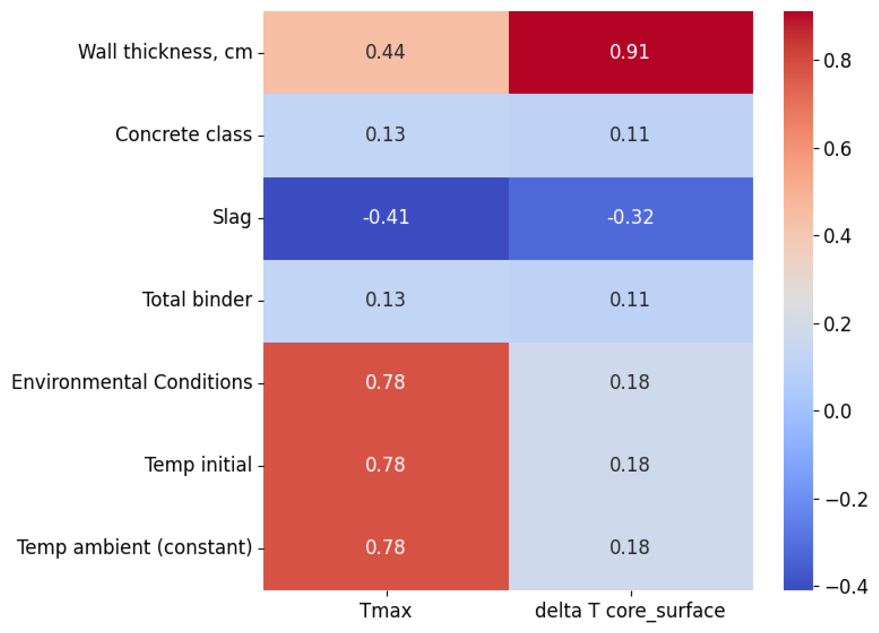
To gain deeper insight into the influence of individual input features on the target variables, a linear correlation analysis was conducted, with the results presented in Figure 6. The correlation matrix displays the Pearson correlation coefficients for each feature-target variable pair, specifically for Tmax and ΔT core_surface.

The analysis revealed that wall thickness had the strongest correlation with ΔT core_surface, with a Pearson coefficient of 0.91, indicating a very strong positive relationship. This variable also showed a moderate correlation with Tmax, at 0.44. For Tmax, environmental conditions, specifically the initial concrete temperature and ambient temperature, also demonstrated a strong positive correlation, each with a coefficient of 0.78, highlighting their significant influence on predicting the maximum internal temperature of concrete.

In contrast, slag content exhibited a negative correlation with both Tmax (−0.41) and ΔT core_surface (−0.32), confirming that higher slag content tends to reduce the thermal effects associated with cement hydration. Other variables, such as concrete class and total binder content, showed low correlation coefficients (approximately 0.11–0.13), suggesting a limited impact on the target variables within the scope of the analysed dataset. It should be clarified that the concrete class is directly related to the amount of cement binder. Based on practical experience, experimental research, and CIRIA C766 guidelines, it is known that higher cement content leads to increased self-heating, with approximately a 10 °C rise under adiabatic conditions per 100 kg of cement. However, this effect is less pronounced in our dataset due to the relatively small variation in concrete classes and binder content, which, however, reflects actual engineering applications. At the same time, larger variations were considered in wall thickness and external conditions, which had a greater influence on the results. Therefore, for the analysed dataset, the feature importance results showing minimal contribution of concrete class and binder content, particularly for the temperature difference between the core and the surface of the element (ΔT core_surface), appear reasonable.

3.4. Feature Importance Analysis

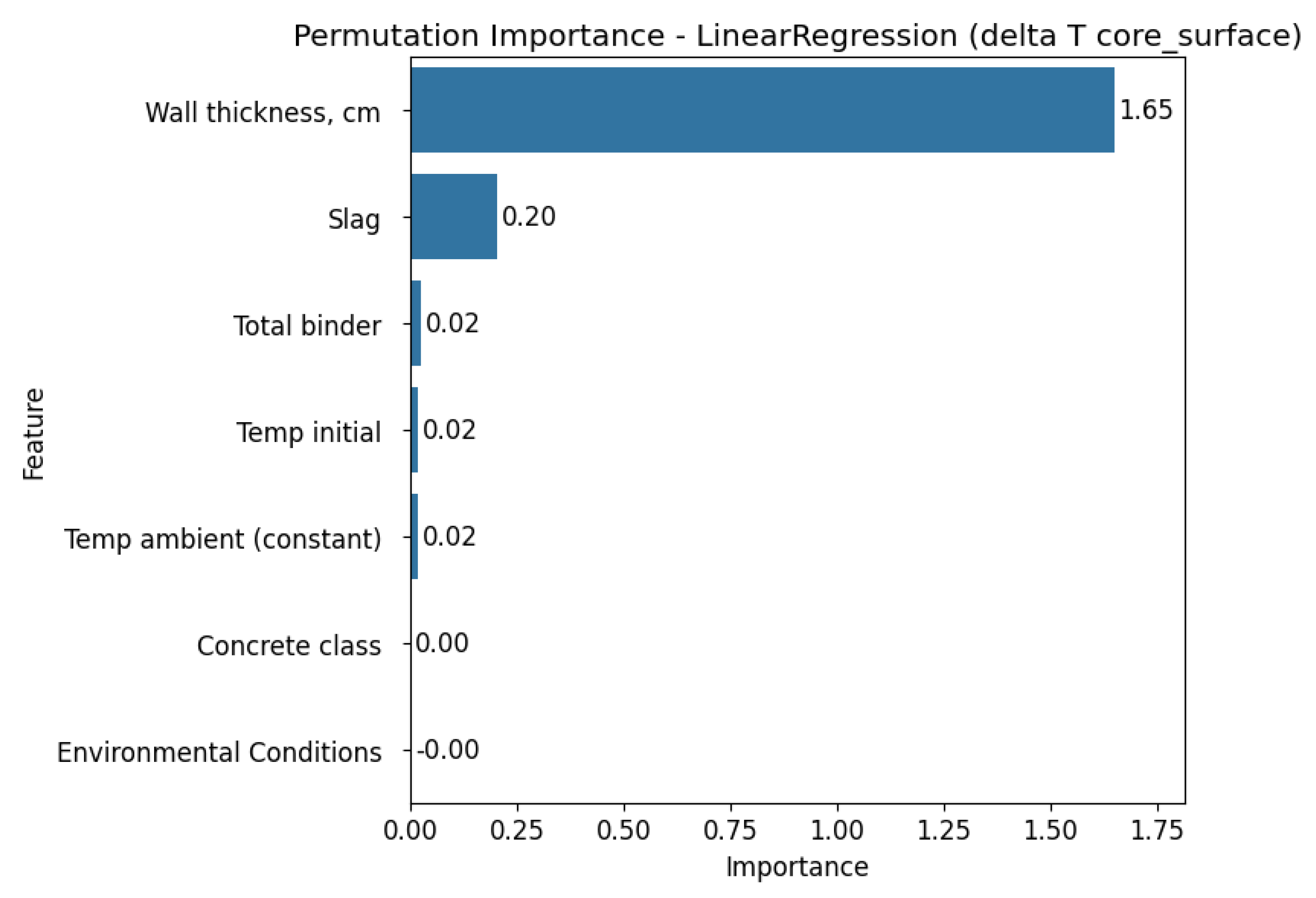
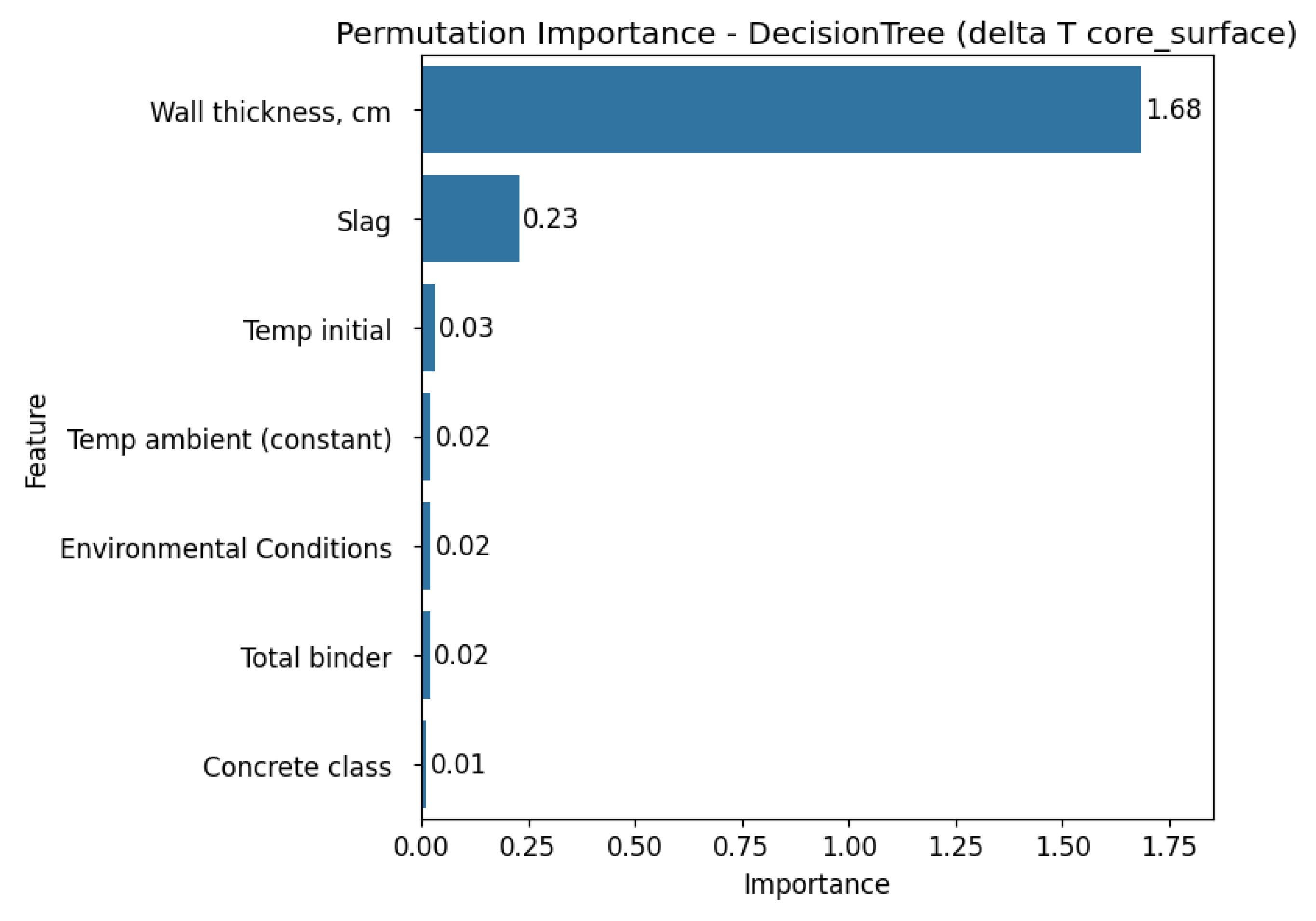
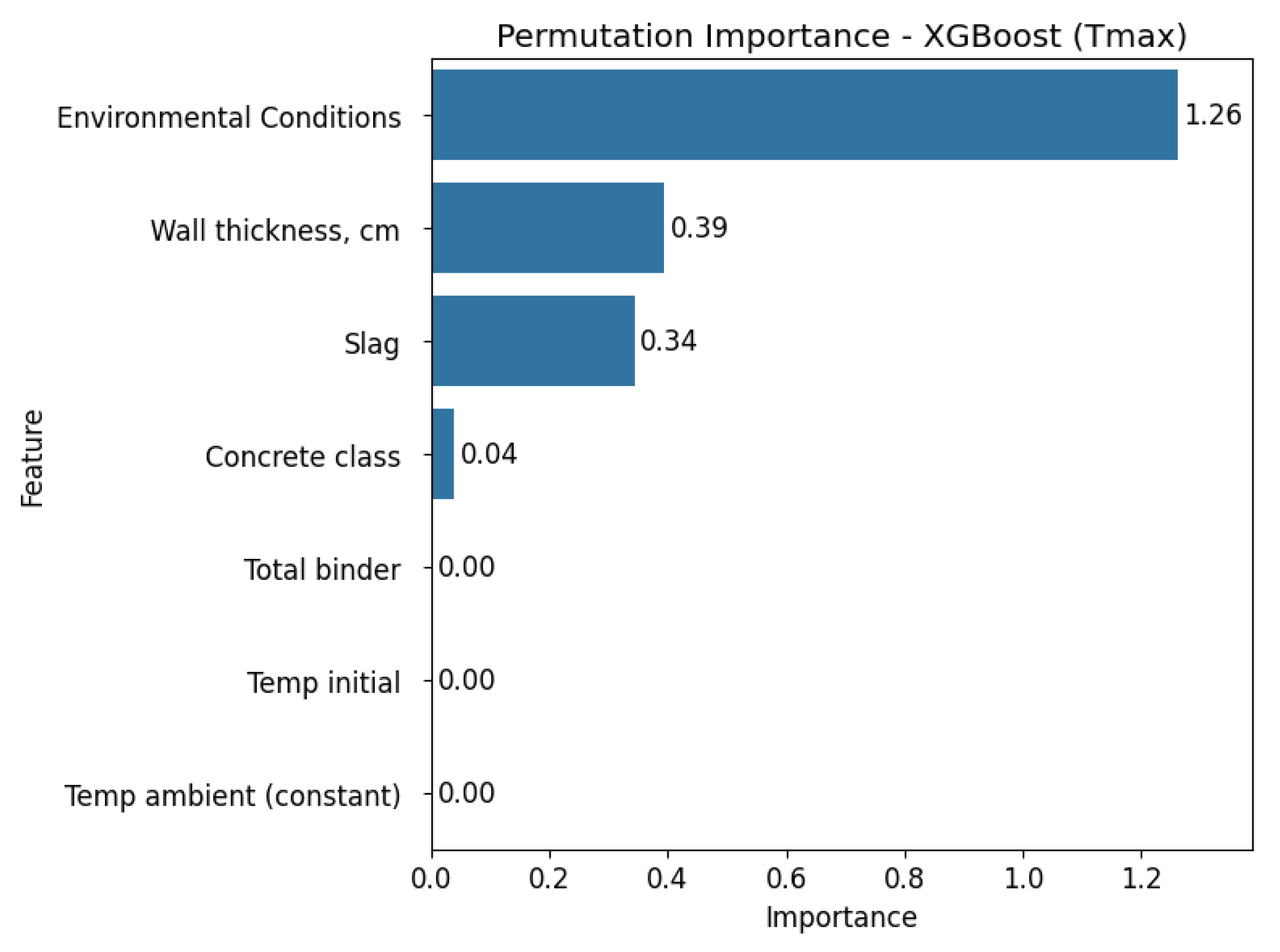
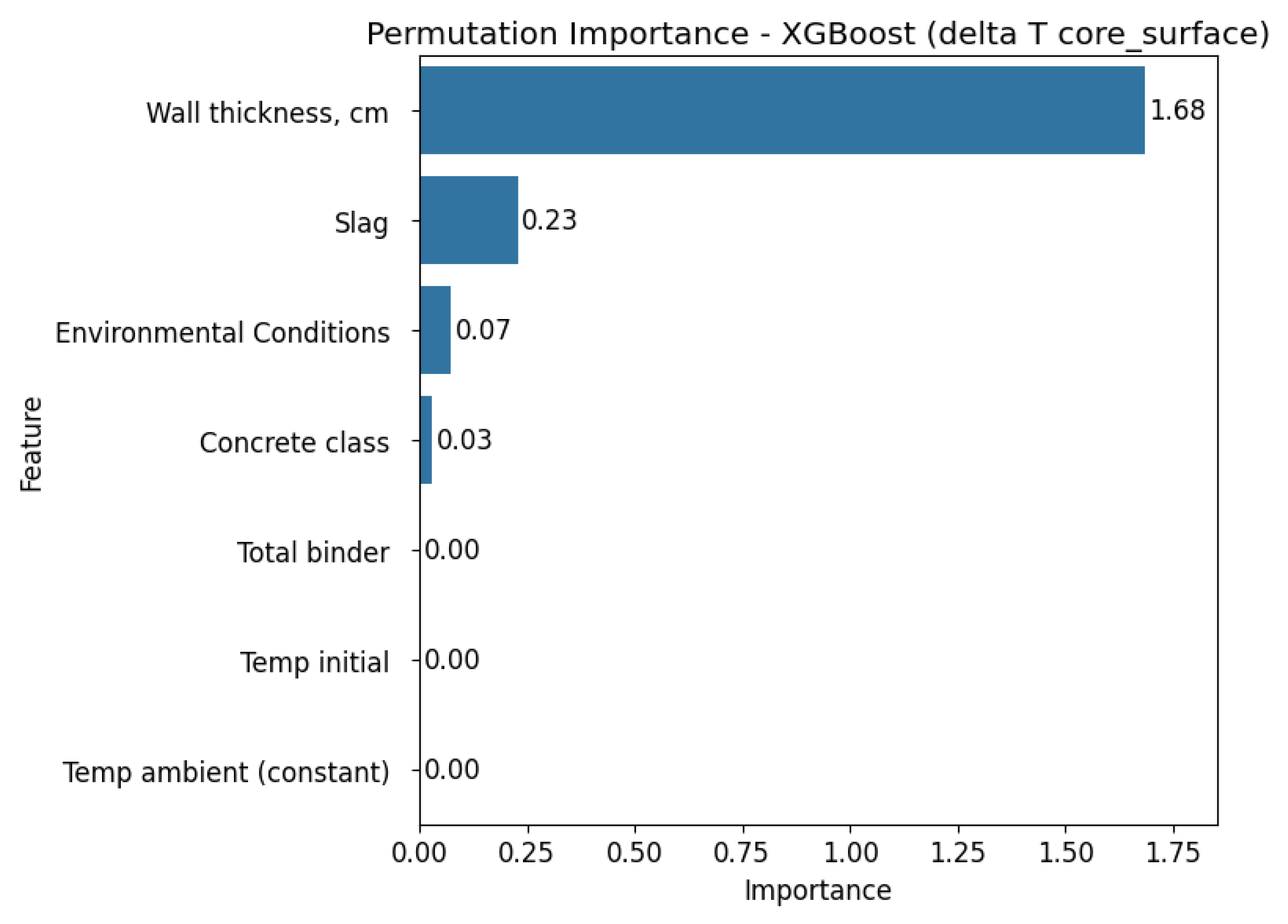
Next, the impact of individual input variables on the prediction quality was assessed using the Permutation Importance analysis method. The results are presented separately for each of the three regression models used in Figure 7, Figure 8, Figure 9, Figure 10, Figure 11 and Figure 12.

The permutation importance analysis conducted across all three models, Linear Regression, Decision Tree, and XGBoost, for the two target variables (Tmax and ΔT core_surface) reveal consistent patterns in feature relevance. Wall thickness consistently stands out as the most influential predictor for ΔT core_surface in all models, showing particularly high importance values in both the Decision Tree and XGBoost models. For Tmax, feature importance varies depending on the model. Linear Regression highlights wall thickness, slag content, initial and ambient temperature as key predictors.

In contrast, the Decision Tree model identifies ambient temperature as the most dominant factor, while XGBoost assigns the greatest importance to environmental conditions overall. Across all models and target variables, certain features such as total binder, concrete class, and environmental conditions consistently show small importance, suggesting limited predictive value in the studied context.

Overall, these findings highlight the critical role of thermal and geometric parameters, particularly wall thickness, in determining both maximum temperature and thermal gradients within concrete structures. However, it is important to emphasise that although the results are generally consistent with existing knowledge about the influence of technological and material factors on concrete hardening temperatures, they are based on the specific dataset used in this analysis.

3.5. Prediction vs. Actual and Residuals Analysis

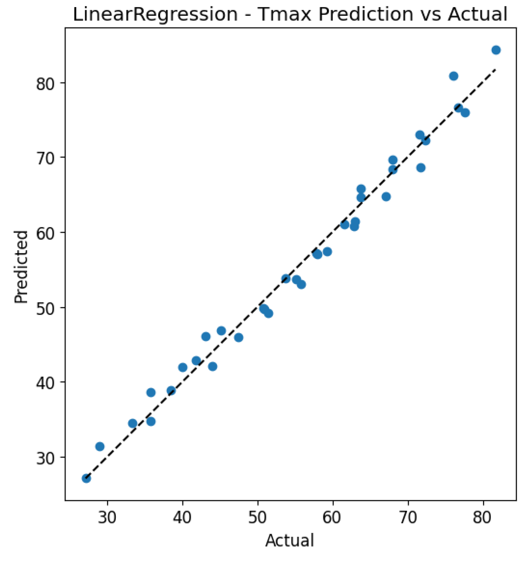
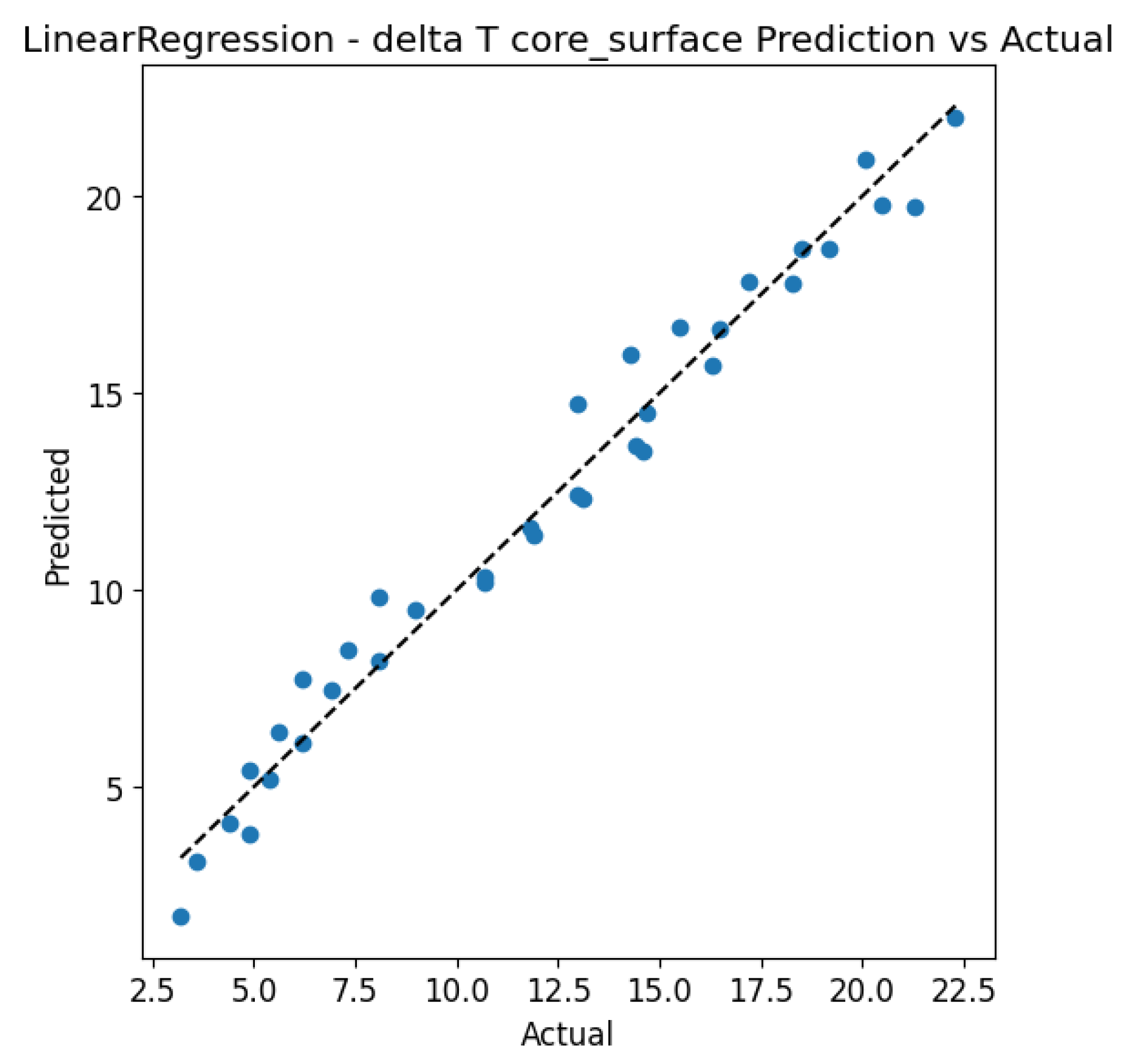
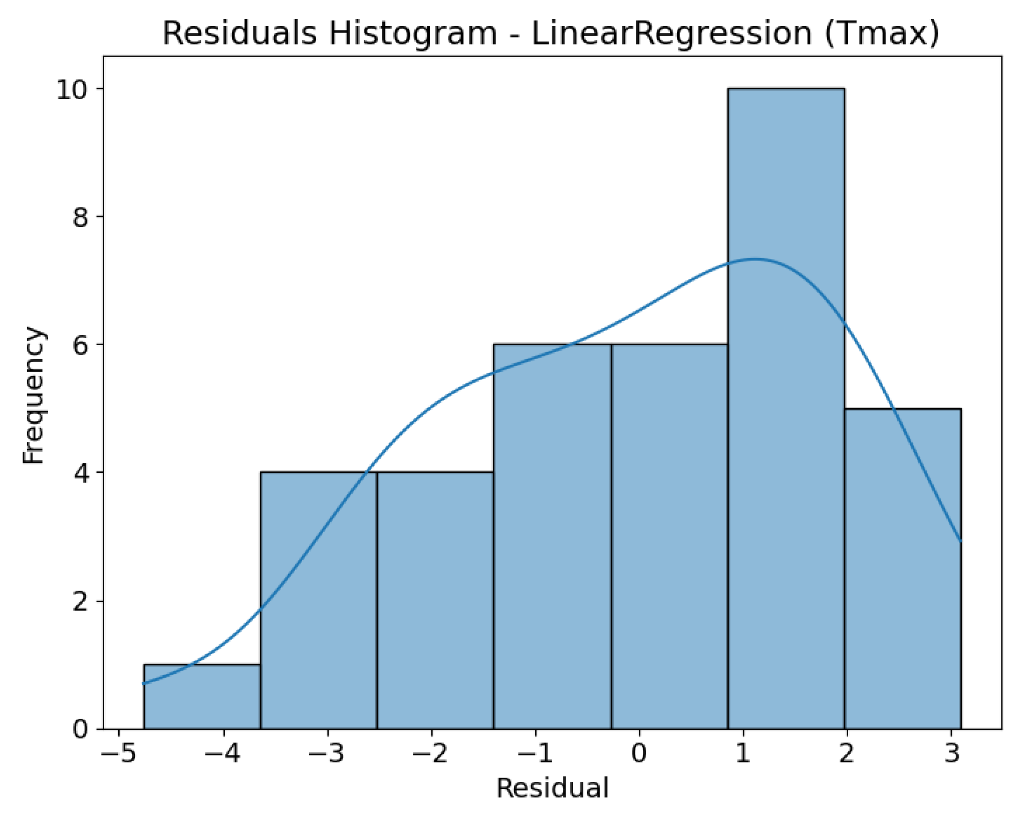
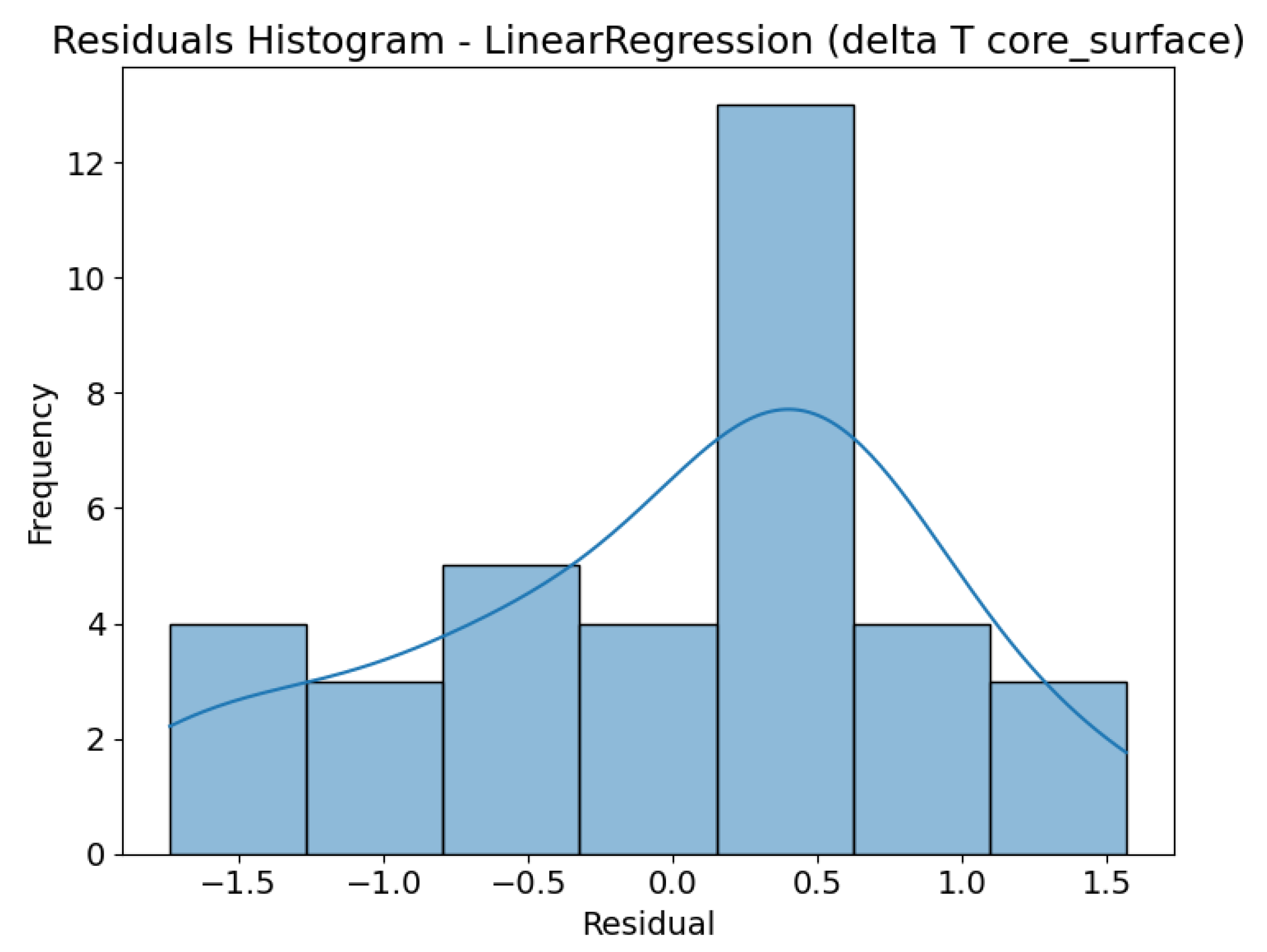
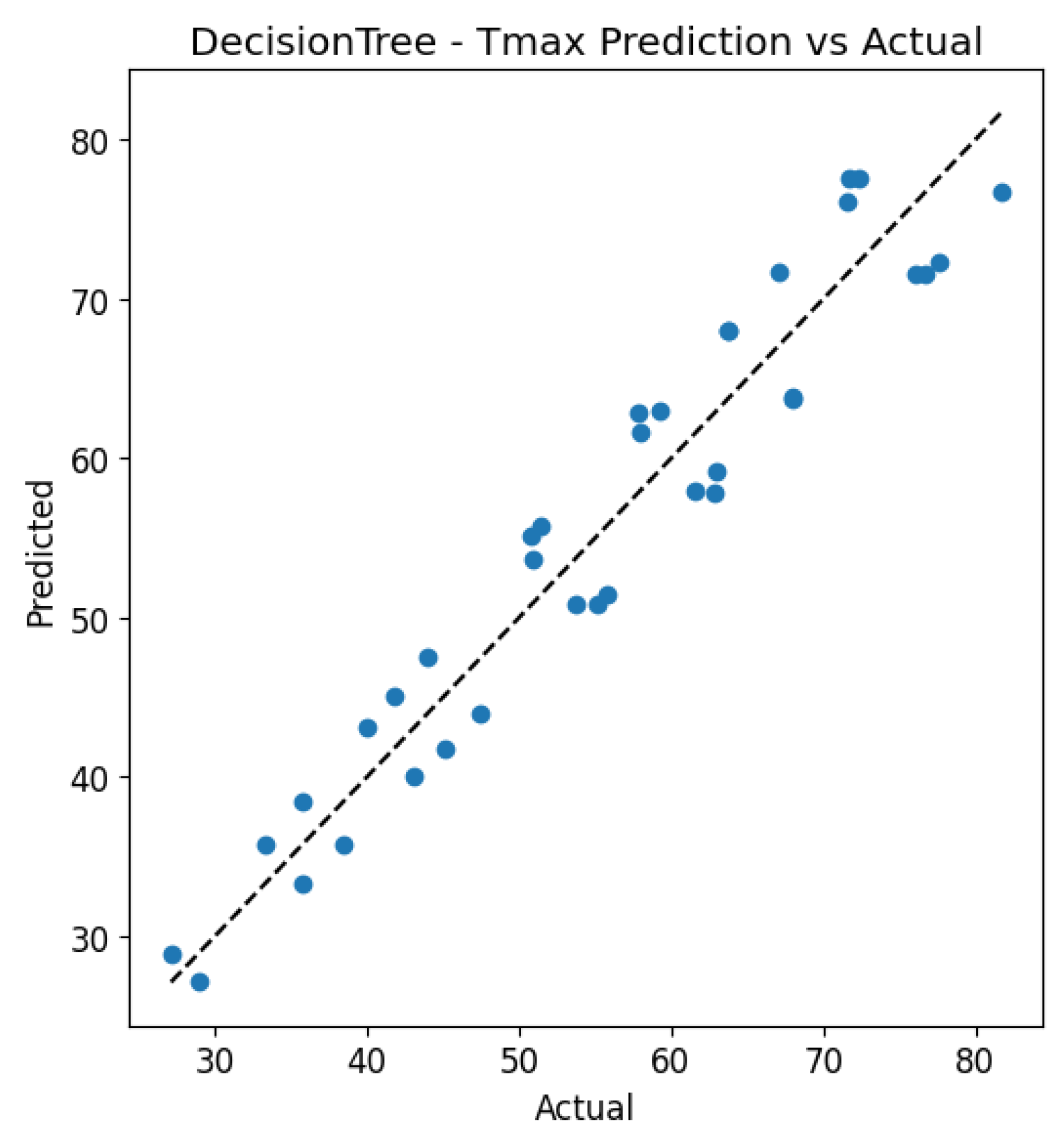
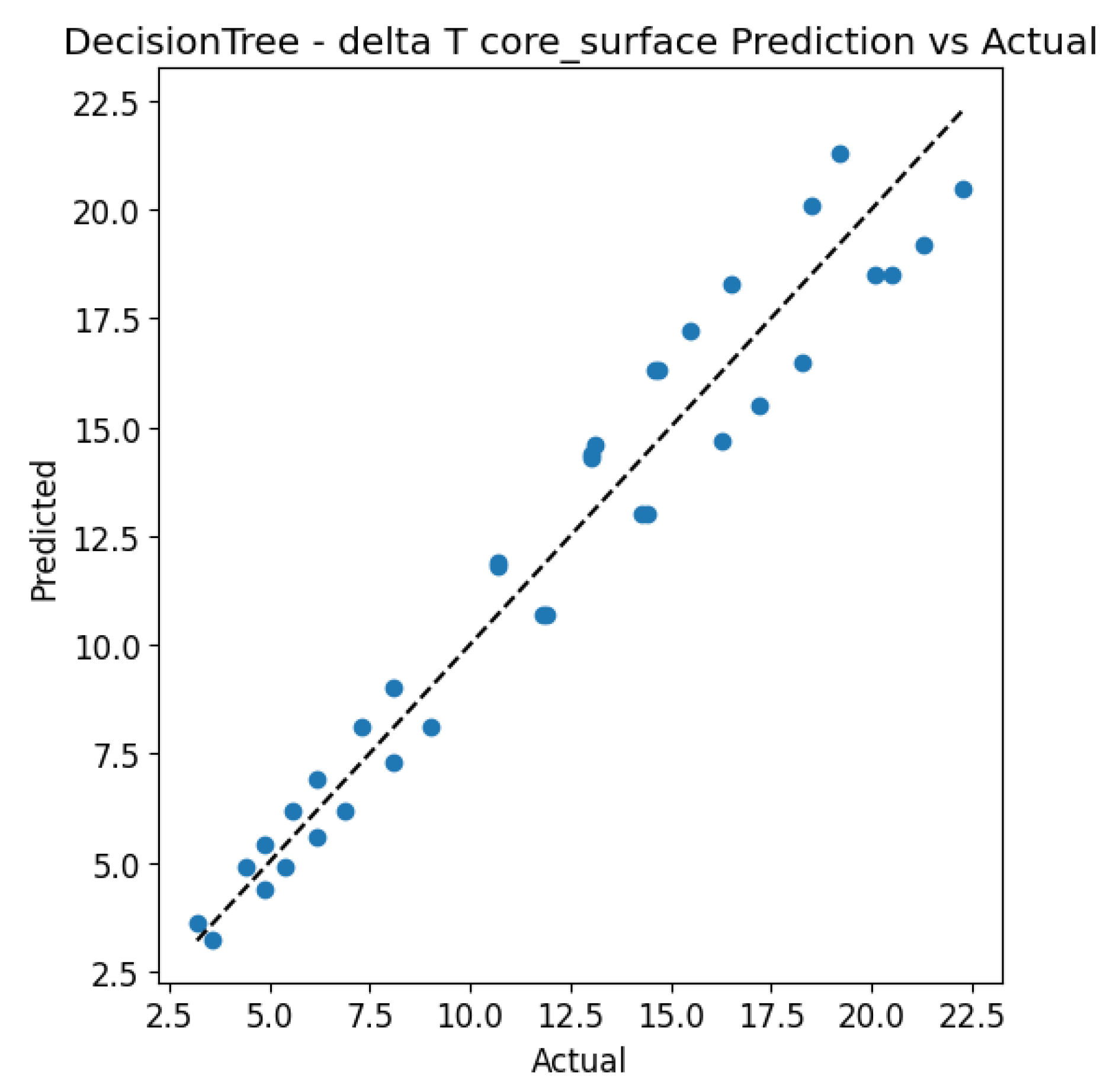
To evaluate prediction accuracy and model calibration, scatter plots comparing predicted versus actual values, along with residual histograms derived from Leave-One-Out cross-validation (LOOCV) results, were analysed. This approach enables the identification of potential systematic errors and provides insight into the distribution of prediction errors relative to the observed data. For the linear regression model (Figure 13, Figure 14, Figure 15 and Figure 16), a high level of agreement was observed between the actual and predicted values, as illustrated by the scatter plots for both target variables. Predictions for ΔT core_surface show very good calibration relative to the ideal line (y = x), while for Tmax, a slight dispersion is visible at higher temperature values. The histograms of residuals indicate that, for ΔT core_surface, the error distribution is relatively symmetric and centred around zero, confirming the absence of significant bias. In contrast, for Tmax, a predominance of positive residuals is evident, suggesting a tendency of the model to overestimate the maximum temperature.

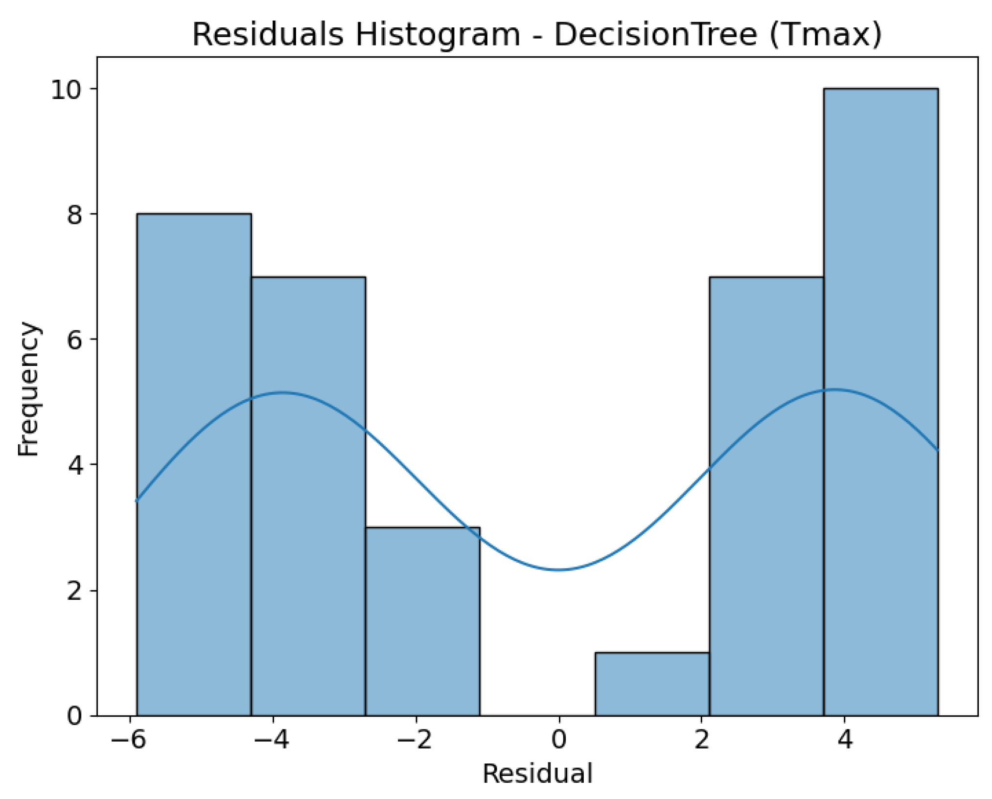
In the case of the Decision Tree model (Figure 17, Figure 18, Figure 19 and Figure 20), prediction accuracy was noticeably lower compared to the other models. The scatter plots reveal greater deviations from the ideal line (y = x), confirming the presence of significant prediction errors, particularly at higher actual values.

The residual histogram for Tmax displays a bimodal distribution, indicating instability in the model’s predictions—frequently alternating between overestimation and underestimation. This bimodal shape is a consequence of the discrete nature of decision trees, which generate predictions in distinct value ranges, leading to clustered residuals. For ΔT core_surface, the residuals show a more uniform distribution; however, the deviation from a normal distribution suggests that the model struggles to fully capture the underlying data patterns.

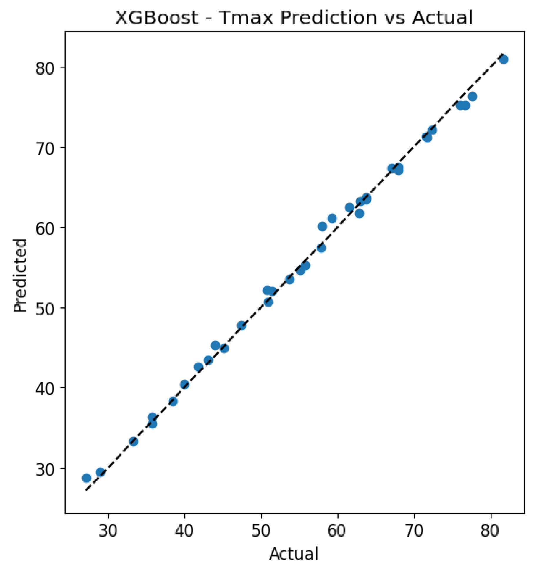
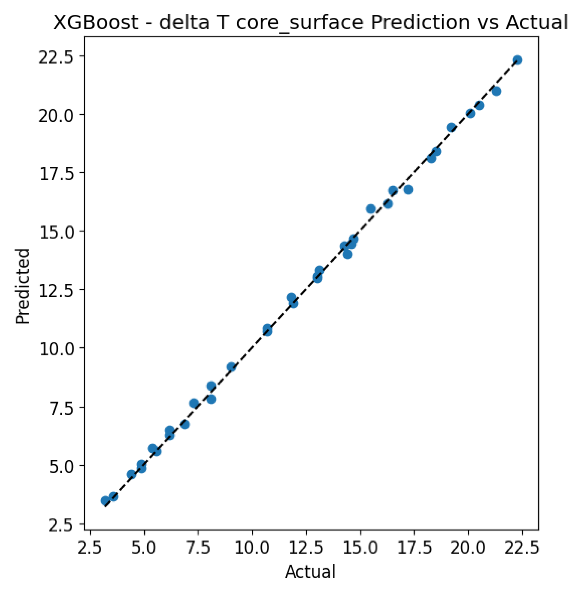
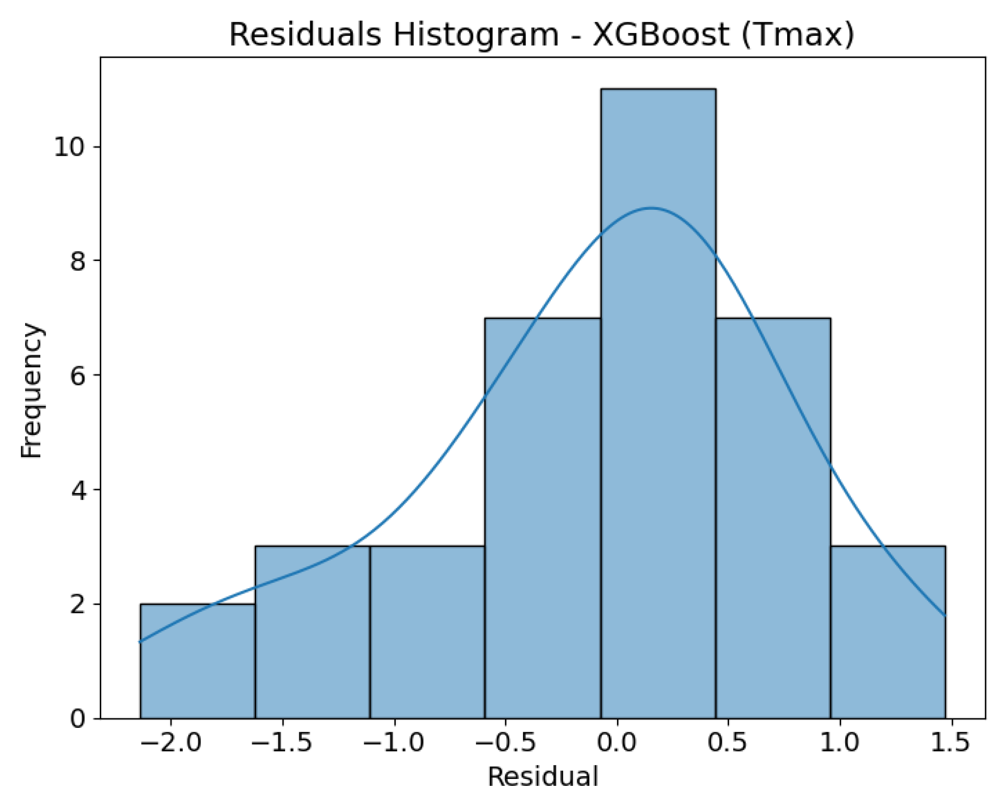
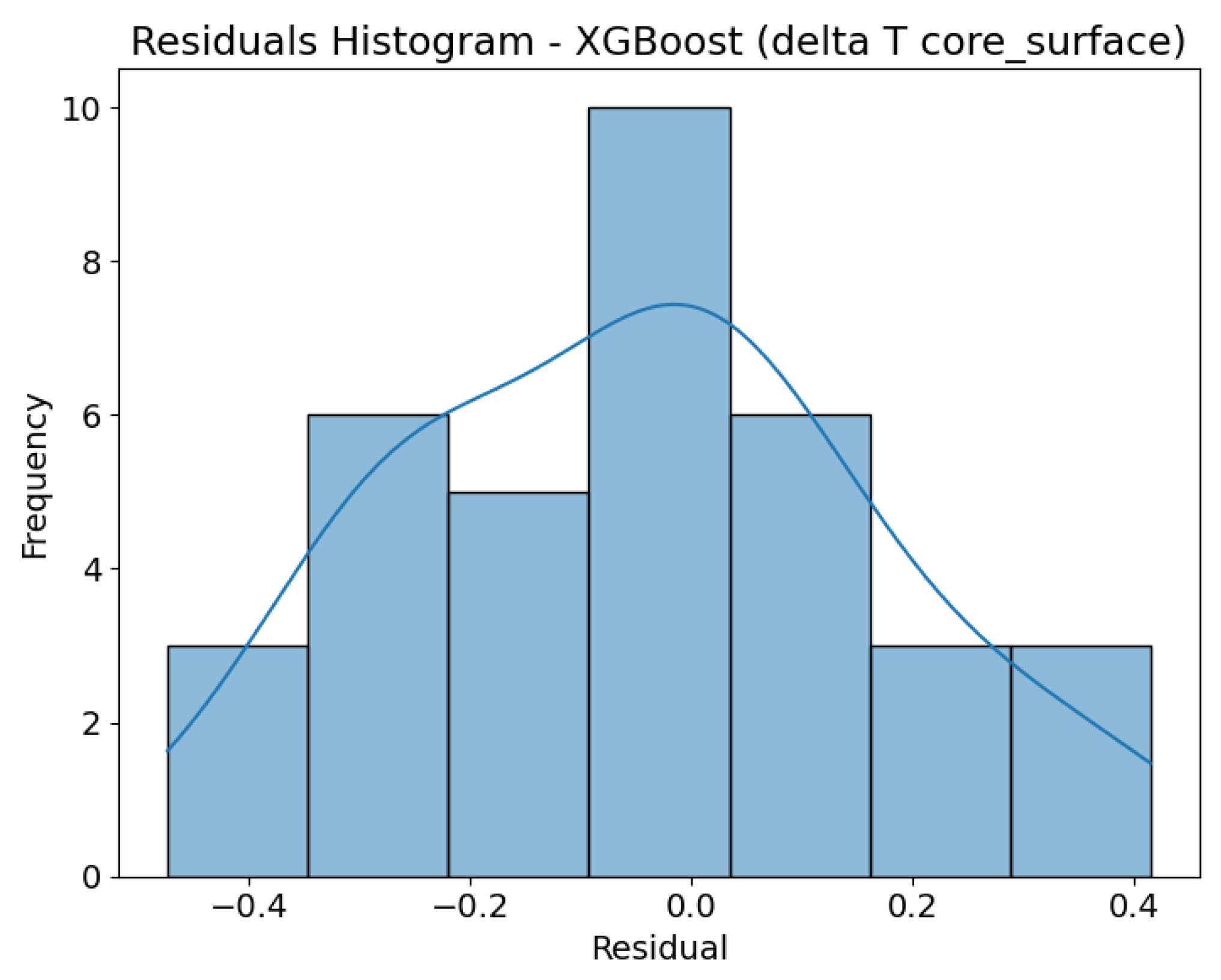
The XGBoost model (Figure 21, Figure 22, Figure 23 and Figure 24) demonstrated the highest predictive accuracy among all the algorithms evaluated. The scatter plots for both target variables show a near-perfect alignment with the y = x line, confirming excellent calibration of the model. The residual histograms exhibit a symmetrical, narrow distribution centred around zero for both variables, indicating high prediction stability and precision. In the case of ΔT core_surface, the errors are particularly minimal and evenly distributed, further confirming the model’s strong ability to capture the underlying relationships in the data.

3.6. Residual Diagnostics

The residual analysis was complemented with statistical tests to confirm the visual findings. Normality of the residual distribution was assessed using the Shapiro–Wilk and D’Agostino–Pearson tests, while potential systematic error (bias) was evaluated with a one-sample t-test (testing whether the residual mean equals zero). The results are summarised in

Table 7. Results of statistical tests for model residuals.

Model	Target Variable	Shapiro p	D’Agostin p	t-Test p	Mean Residual
Linear Regression	Tmax	0.3352	0.4372	0.9073	−0.037
Linear Regression	ΔT core_surface	0.0872	0.3997	0.9433	−0.011
Decision Tree	Tmax	0.0001	0.0000	0.9869	−0.011
Decision Tree	ΔT core_surface	0.0121	0.0001	0.9406	0.017
XGBoost	Tmax	0.3054	0.3060	0.4645	−0.105
XGBoost	ΔT core_surface	0.8648	0.7589	0.1800	−0.049

.

For the LinearRegression model, the residuals did not significantly deviate from normality, and their mean was close to zero, indicating no detectable bias. For the DecisionTree model, the tests revealed a deviation from normality, although the residual mean was not significantly different from zero. The bimodal shape of the residual histogram reflects the discrete nature of tree-based predictions. In contrast, for the XGBoost model, the residuals followed a distribution consistent with normality and were centred around zero, confirming that the ensemble method effectively smooths the irregularities observed in a single tree.

4. Conclusions

This study developed and compared three machine learning regression models to predict the thermal response of massive concrete, focusing on two key parameters: the maximum temperature (Tmax) and the temperature difference between the concrete core and surface (ΔT core_surface). The models were trained on the data, incorporating both cross-section dimensions of the analysed wall, concrete mix properties and environmental conditions.

The results demonstrated that the XGBoost model achieved the highest predictive accuracy, with coefficient of determination (R²) values of 0.997 for Tmax and 0.998 for ΔT core_surface, outperforming both the linear regression and Decision Tree models. Residual analysis and scatter plots confirmed the high stability and excellent calibration of the XGBoost predictions. The linear regression model also delivered satisfactory performance, particularly for Tmax prediction, with a low mean absolute percentage error (MAPE) of 3.01%. However, for ΔT core_surface, the error increased significantly (MAPE = 8.32%), suggesting the model’s limited capacity to capture nonlinear relationships within the data.

The Decision Tree model showed the lowest predictive performance among the three. Its residual distributions revealed signs of instability and greater error dispersion, while its R² values and error metrics (MAE, MAPE) were notably worse than those of the other models.

These findings confirm that properly configured machine learning algorithms, especially gradient boosting methods like XGBoost, can serve as powerful tools for analysing thermal behaviour and heat transfer in massive concrete structures. Hence, the ML models may provide a systematic framework for predicting early age thermal behaviour in mass concrete structures. Once an appropriate ML model is selected and tested, and the database is expanded, it could form the basis of a practical tool for users to predict temperature development based on a broad dataset of input parameters. This study primarily explores the potential of such an approach, as no comprehensive attempts of this kind currently exist. This methodology may also allow engineers to assess the relative importance of technological and material factors influencing temperature development in the specific concrete structure, supporting better-informed design decisions and thermal control strategies.

References

1. ACI Committee. ACI 207.1R-05—Guide to Mass Concrete; American Concrete Institute: Farmington Hills, MI, USA, 2005. [Google Scholar]
2. ACI Committee. ACI 207.2R-07—Report on Thermal and Volume Change Effects on Cracking of Mass Concrete; American Concrete Institute: Farmington Hills, MI, USA, 2007. [Google Scholar]
3. Bamforth, P.B. Construction Industry Research and Information Association Control of Cracking Caused by Restrained Deformation in Concrete. CIRIA C766; Construction Industry Research and Information Association: London, UK, 2018. [Google Scholar]
4. Azenha, M.; Faria, R.; Ferreira, D. Identification of Early-Age Concrete Temperatures and Strains: Monitoring and Numerical Simulation. Cem. Concr. Compos. 2009, 31, 369–378. [Google Scholar] [CrossRef]
5. Maruyama, I.; Lura, P. Properties of Early-Age Concrete Relevant to Cracking in Massive Concrete. Cem. Concr. Res. 2019, 123, 105770. [Google Scholar] [CrossRef]
6. Schindler, A.K.; Folliard, K.J. Heat of Hydration Models for Cementitious Materials. Mater. J. 2005, 102, 24–33. [Google Scholar] [CrossRef]
7. Branco, F.A.; Mendes, P.; Mirambell, E. Heat of Hydration Effects in Concrete Structures. Mater. J. 1992, 89, 139–145. [Google Scholar] [CrossRef]
8. Baran, T.; Pichniarczyk, P. Correlation Factor between Heat of Hydration and Compressive Strength of Common Cement. Constr. Build. Mater. 2017, 150, 321–332. [Google Scholar] [CrossRef]
9. Bourchy, A.; Barnes, L.; Bessette, L.; Chalencon, F.; Joron, A.; Torrenti, J.M. Optimization of Concrete Mix Design to Account for Strength and Hydration Heat in Massive Concrete Structures. Cem. Concr. Compos. 2019, 103, 233–241. [Google Scholar] [CrossRef]
10. de Matos, P.R.; Junckes, R.; Graeff, E.; Prudêncio, L.R., Jr. Effectiveness of Fly Ash in Reducing the Hydration Heat Release of Mass Concrete. J. Build. Eng. 2020, 28, 101063. [Google Scholar] [CrossRef]
11. Hong, Y.; Lin, J.; Chen, W. Simulation of Thermal Field in Mass Concrete Structures with Cooling Pipes by the Localized Radial Basis Function Collocation Method. Int. J. Heat Mass Transf. 2019, 129, 449–459. [Google Scholar] [CrossRef]
12. Klemczak, B. Prediction of Coupled Heat and Moisture Transfer in Early-Age Massive Concrete Structures. Numer. Heat Transf. Part A Appl. 2011, 60, 212–233. [Google Scholar] [CrossRef]
13. Klemczak, B.; Batog, M.; Giergiczny, Z.; Żmij, A. Complex Effect of Concrete Composition on the Thermo-Mechanical Behaviour of Mass Concrete. Materials 2018, 11, 2207. [Google Scholar] [CrossRef]
14. Ma, R.; Zhang, F.; Li, Q.; Hu, Y.; Liu, Z.; Tan, Y.; Zhang, Q. Intelligent Optimal Strategy for Balancing Safety–Quality–Efficiency–Cost in Massive Concrete Construction. Intell. Infrastruct. Constr. 2025, 1, 2. [Google Scholar] [CrossRef]
15. Klemczak, B.; Smolana, A.; Jędrzejewska, A. Modeling of Heat and Mass Transfer in Cement-Based Materials during Cement Hydration—A Review. Energies 2024, 17, 2513. [Google Scholar] [CrossRef]
16. Jędrzejewska, A.; Benboudjema, F.; Lacarrière, L.; Azenha, M.; Schlicke, D.; Dal Pont, S.; Delaplace, A.; Granja, J.; Hájková, K.; Joachim Heinrich, P.; et al. COST TU1404 Benchmark on Macroscopic Modelling of Concrete and Concrete Structures at Early Age: Proof-of-Concept Stage. Constr. Build. Mater. 2018, 174, 173–189. [Google Scholar] [CrossRef]
17. Jędrzejewska, A.; Kanavaris, F.; Zych, M.; Schlicke, D.; Azenha, M. Experiences on Early Age Cracking of Wall-on-Slab Concrete Structures. Structures 2020, 27, 2520–2549. [Google Scholar] [CrossRef]
18. Fairbairn, E.M.R.; Azenha, M. Thermal Cracking of Massive Concrete Structures. State of the Art Report of the RILEM Technical Committee 254-CMS; Springer: Cham, Switzerland, 2018; ISBN 978-3-319-76616-4. [Google Scholar]
19. Bergman, T.L.; Lavine, A.S.; Incropera, F.P. Fundamentals of Heat and Mass Transfer, 7th ed.; John Wiley & Sons, Incorporated: Hoboken, NJ, USA, 2011; ISBN 978-1-118-13725-3. [Google Scholar]
20. Gawin, D.; Pesavento, F.; Schrefler, B.A. Hygro-Thermo-Chemo-Mechanical Modelling of Concrete at Early Ages and beyond. Part I: Hydration and Hygro-Thermal Phenomena. Int. J. Numer. Methods Eng. 2006, 67, 299–331. [Google Scholar] [CrossRef]
21. Honorio, T.; Bary, B.; Benboudjema, F. Evaluation of the Contribution of Boundary and Initial Conditions in the Chemo-Thermal Analysis of a Massive Concrete Structure. Eng. Struct. 2014, 80, 173–188. [Google Scholar] [CrossRef]
22. Kwak, H.-G.; Ha, S.-J.; Kim, J.-K. Non-Structural Cracking in RC Walls: Part I. Finite Element Formulation. Cem. Concr. Res. 2006, 36, 749–760. [Google Scholar] [CrossRef]
23. Di Luzio, G.; Cusatis, G. Hygro-Thermo-Chemical Modeling of High-Performance Concrete. II: Numerical Implementation, Calibration, and Validation. Cem. Concr. Compos. 2009, 31, 309–324. [Google Scholar] [CrossRef]
24. Aurich, M.; Campos Filho, A.; Bittencourt, T.N.; Shah, S.P. Finite Element Modeling of Concrete Behavior at Early Age. Rev. IBRACON Estrut. Mater. 2009, 2, 37–58. [Google Scholar] [CrossRef]
25. Zreiki, J.; Bouchelaghem, F.; Chaouche, M. Early-Age Behaviour of Concrete in Massive Structures, Experimentation and Modelling. Nucl. Eng. Des. 2010, 240, 2643–2654. [Google Scholar] [CrossRef]
26. Briffaut, M.; Benboudjema, F.; Torrenti, J.-M.; Nahas, G. Effects of Early-Age Thermal Behaviour on Damage Risks in Massive Concrete Structures. Eur. J. Environ. Civ. Eng. 2012, 16, 589–605. [Google Scholar] [CrossRef]
27. Faria, R.; Azenha, M.; Figueiras, J.A. Modelling of Concrete at Early Ages: Application to an Externally Restrained Slab. Cem. Concr. Compos. 2006, 28, 572–585. [Google Scholar] [CrossRef]
28. Azenha, M. Numerical Simulation of the Structural Behaviour of Concrete Since Its Early Ages. Ph.D. Thesis, University of Porto, Porto, Portugal, 2009. [Google Scholar]
29. Smolana, A.; Klemczak, B.; Azenha, M.; Schlicke, D. Early Age Cracking Risk in a Massive Concrete Foundation Slab: Comparison of Analytical and Numerical Prediction Models with on-Site Measurements. Constr. Build. Mater. 2021, 301, 124135. [Google Scholar] [CrossRef]
30. Azenha, M.; Sousa, C.; Faria, R.; Neves, A. Thermo–Hygro–Mechanical Modelling of Self-Induced Stresses during the Service Life of RC Structures. Eng. Struct. 2011, 33, 3442–3453. [Google Scholar] [CrossRef]
31. Madea, B.; Rödig, A. Time of Death Dependent Criteria in Vitreous Humor—Accuracy of Estimating the Time since Death. Forensic Sci. Int. 2006, 164, 87–92. [Google Scholar] [CrossRef]
32. Roustaei, N. Application and Interpretation of Linear-Regression Analysis. Med. Hypothesis Discov. Innov. Ophthalmol. 2024, 13, 151–159. [Google Scholar] [CrossRef]
33. Mienye, I.D.; Jere, N. A Survey of Decision Trees: Concepts, Algorithms, and Applications. IEEE Access 2024, 12, 86716–86727. [Google Scholar] [CrossRef]
34. Niazkar, M.; Menapace, A.; Brentan, B.; Piraei, R.; Jimenez, D.; Dhawan, P.; Righetti, M. Applications of XGBoost in Water Resources Engineering: A Systematic Literature Review (Dec 2018–May 2023). Environ. Model. Softw. 2024, 174, 105971. [Google Scholar] [CrossRef]
35. Ilc, A.; Turk, G.; Kavčič, F.; Trtnik, G. New Numerical Procedure for the Prediction of Temperature Development in Early Age Concrete Structures. Autom. Constr. 2009, 18, 849–855. [Google Scholar] [CrossRef]
36. Liu, D.; Zhang, W.; Tang, Y.; Jian, Y. Prediction of Hydration Heat of Mass Concrete Based on the SVR Model. IEEE Access 2021, 9, 62935–62945. [Google Scholar] [CrossRef]
37. Jiang, Y.; Zuo, W.; Yuan, C.; Xu, G.; Wei, X.; Zhang, J.; She, W. Deep Learning Approaches for Prediction of Adiabatic Temperature Rise of Concrete with Complex Mixture Constituents. J. Build. Eng. 2023, 73, 106816. [Google Scholar] [CrossRef]
38. Kekez, S.; Krzywoń, R. Prediction of Bonding Strength of Externally Bonded SRP Composites Using Artificial Neural Networks. Materials 2022, 15, 1314. [Google Scholar] [CrossRef]
39. Kekez, S.; Kubica, J. Application of Artificial Neural Networks for Prediction of Mechanical Properties of CNT/CNF Reinforced Concrete. Materials 2021, 14, 5637. [Google Scholar] [CrossRef]
40. Zheng, M.; Fan, X.; Li, C.; Li, J.; He, D.; Zhu, R. Machine Learning-Based Recursive Prediction and Application of Green’s Function of Water-Wave Radiation and Diffraction. J. Mar. Sci. Eng. 2025, 13, 1488. [Google Scholar] [CrossRef]
41. Akbas, M. Integrated GBR–NSGA-II Optimization Framework for Sustainable Utilization of Steel Slag in Road Base Layers. Appl. Sci. 2025, 15, 8516. [Google Scholar] [CrossRef]
42. Džolev, I.; Kekez-Baran, S.; Rašeta, A. Fire Resistance of Steel Beams with Intumescent Coating Exposed to Fire Using ANSYS and Machine Learning. Buildings 2025, 15, 2334. [Google Scholar] [CrossRef]
43. Wu, F.; Zhu, J.; Yang, H.; He, X.; Peng, Q. Data-Driven Symmetry and Asymmetry Investigation of Vehicle Emissions Using Machine Learning: A Case Study in Spain. Symmetry 2025, 17, 1223. [Google Scholar] [CrossRef]
44. DeRousseau, M.A.; Kasprzyk, J.R.; Srubar, W.V. Computational Design Optimization of Concrete Mixtures: A Review. Cem. Concr. Res. 2018, 109, 42–53. [Google Scholar] [CrossRef]
45. Blockeel, H.; Devos, L.; Frénay, B.; Nanfack, G.; Nijssen, S. Decision Trees: From Efficient Prediction to Responsible AI. Front. Artif. Intell. 2023, 26, 4553. [Google Scholar] [CrossRef]
Figure 1. Factors affecting heat transfer and temperature rise in mass concrete.
Energies 18 04673 g001
Figure 2. Data Collection scheme.
Energies 18 04673 g002
Figure 3. Data Collection set: (a) maximum internal temperature (Tmax), (b) temperature difference between the wall’s interior and exterior surfaces (ΔT core_surface).
Energies 18 04673 g003
Figure 4. Histograms of input and output variables.
Energies 18 04673 g004
Figure 5. Data Processing Flowchart.
Energies 18 04673 g005
Figure 6. Heatmap showing Pearson correlation coefficients between input features and target variables (Tmax and ΔT core_surface).
Energies 18 04673 g006
Figure 7. Permutation importance of input features for the Linear Regression model (Tmax).
Energies 18 04673 g007
Figure 8. Permutation importance of input features for the Linear Regression model (ΔT core_surface).
Energies 18 04673 g008
Figure 9. Permutation importance of input features for the Decision Tree model (Tmax).
Energies 18 04673 g009
Figure 10. Permutation importance of input features for the Decision Tree model (ΔT core_surface).
Energies 18 04673 g010
Figure 11. Permutation importance of input features for the XGBoost model (Tmax).
Energies 18 04673 g011
Figure 12. Permutation importance of input features for the XGBoost model (ΔT core_surface).
Energies 18 04673 g012
Figure 13. Scatter plot of predicted vs. actual Tmax values using the Linear Regression model.
Energies 18 04673 g013
Figure 14. Scatter plot of predicted vs. actual ΔT core_surface values using the Linear Regression model.
Energies 18 04673 g014
Figure 15. Histogram of residuals for Tmax predicted by the Linear Regression model.
Energies 18 04673 g015
Figure 16. Histogram of residuals for ΔT core_surface in the Linear Regression model.
Energies 18 04673 g016
Figure 17. Scatter plot of predicted vs. actual Tmax values using the Decision Tree model.
Energies 18 04673 g017
Figure 18. Scatter plot of predicted vs. actual ΔT core_surface values using the Decision Tree model.
Energies 18 04673 g018
Figure 19. Histogram of residuals for Tmax predicted by the Decision Tree model.
Energies 18 04673 g019
Figure 20. Histogram of residuals for ΔT core_surface in the Decision Tree model.
Energies 18 04673 g020
Figure 21. Scatter plot of predicted vs. actual Tmax values using the XGBoost model.
Energies 18 04673 g021
Figure 22. Scatter plot of predicted vs. actual ΔT core_surface values using the XGBoost model.
Energies 18 04673 g022
Figure 23. Histogram of residuals for Tmax predicted by the XGBoost model.
Energies 18 04673 g023
Figure 24. Histogram of residuals for ΔT core_surface in the XGBoost model.
Energies 18 04673 g024