Article

Dynamic Behavior of a Glazing System and Its Impact on Thermal Comfort: Short-Term In Situ Assessment and Machine Learning-Based Predictive Modeling

by
Saman Abolghasemi Moghaddam
1,2,*,
Nuno Simões
2,3,*,
Michael Brett
2,3,
Manuel Gameiro da Silva
4 and
Joana Prata
2,3
1
Department of Mechanical Engineering, University Coimbra, Rua Luís Reis Santos, Pólo II, 3030-788 Coimbra, Portugal
2
Itecons—Institute for Research and Technological Development in Construction, Energy, Environment and Sustainability, Rua Pedro Hispano, 3030-289 Coimbra, Portugal
3
CERIS, Department of Civil Engineering, University Coimbra, Rua Luís Reis Santos, Pólo II, 3030-790 Coimbra, Portugal
4
ADAI, Department of Mechanical Engineering, University Coimbra, Rua Luís Reis Santos, Pólo II, 3030-788 Coimbra, Portugal
*
Authors to whom correspondence should be addressed.
Energies 2025, 18(17), 4656; https://doi.org/10.3390/en18174656
Submission received: 31 July 2025 / Revised: 27 August 2025 / Accepted: 29 August 2025 / Published: 2 September 2025

Abstract

In the context of retrofitting existing buildings into nearly zero-energy buildings (NZEBs), in situ assessment methods have proven reliable for evaluating the performance of building components, including glazing systems. However, these methods are often time-consuming, intrusive to occupants, and disruptive to building operations. This study investigates the potential of a machine learning approach—multiple linear regression (MLR)—to predict the dynamic performance of an office building’s glazing system by analyzing surface temperature variations and their impact on nearby thermal comfort. The models were trained using in situ data collected over just two weeks—one in September and one in December—but were applied to predict the glazing performance on multiple other dates with diverse weather conditions. Results show that MLR predictions closely matched nighttime measurements, while some discrepancies occurred during the daytime. Nevertheless, the machine learning model achieved a daytime prediction accuracy of approximately 1.5 °C in terms of root mean square error (RMSE), which is lower than the values reported in previous studies. For thermal comfort evaluation, the MLR model identified the periods with thermal discomfort with an overall accuracy of approximately 92%. However, during periods when the difference between predicted and measured operative temperatures exceeded 1 °C, the thermal comfort predictions showed greater deviation from actual measurements. The study concludes by acknowledging its limitations and recommending a future approach that integrates machine learning with laboratory-based techniques (e.g., hot-box setups and solar simulators) and in situ measurements, together with a broader variety of glazing samples, to more effectively evaluate and enhance prediction accuracy, robustness, and generalizability.

1. Introduction

Around 40% of global energy consumption is attributed to buildings, positioning them among the most energy-intensive sectors. Enhancing the performance of building envelope components is therefore crucial, given their significant role in thermal regulation and overall energy efficiency [1]. As a key element of the envelope, windows notably influence energy performance, aesthetics, and occupant comfort. Their impact varies with climate, building age, type, and size, often making them a primary source of energy loss. Research indicates that windows may account for 20–60% of such losses, while also contributing to unwanted solar heat gain and daylight penetration, which can cause thermal and visual discomfort and elevate heating and cooling demands [2,3,4,5,6,7,8,9]. Glazing, which generally constitutes the majority of a window’s surface area, plays a critical role in determining its thermal performance and thus merits targeted investigation [9,10,11,12]. Studies consistently emphasize the importance of two key metrics—thermal transmittance (U-value) and solar heat gain coefficient (SHGC, also known as g-value)—as they significantly affect both energy efficiency and thermal behavior [2,13,14,15].
Comprehensive reviews by Moghaddam et al. [2,9], Simões et al. [16], and [13] underscore the importance of evaluating glazing systems from two complementary perspectives: (1) standardized steady-state metrics—such as U-value and g-value—which offer essential benchmarks for design and comparison; and (2) the dynamic performance under real-world, variable outdoor conditions. The latter is particularly crucial, as factors like location, orientation, and climate can lead to significant deviations from standardized values, as highlighted by Kuhn [17]. Understanding dynamic behavior also supports the development of advanced building façade components designed to enhance performance and improve resilience to external temperature fluctuations [18,19,20].
One approach to evaluating the dynamic behavior of glazing systems involves the use of validated simulation tools [21,22] that model heat transfer through glazing assemblies. However, these tools depend on precise input data regarding the thermal and optical properties of each glazing layer, which can be challenging to acquire—especially for older systems. Moreover, simulations often rely on theoretical assumptions that may neglect real-world factors such as material aging, degradation, and manufacturing imperfections [2,16].
A practical method for assessing the dynamic performance of existing glazing systems is through extended in situ measurements under varying environmental conditions [16,23]. While effective, this approach is often resource-intensive, potentially disrupting building operations, inconveniencing occupants, and incurring high costs. As a result, there is growing interest in methods that shorten measurement durations without sacrificing accuracy. One such approach involves using short-term measurement data to predict year-round performance, supported by machine learning (ML) techniques. ML models require fewer building-specific inputs [22] and can deliver accurate results within reduced timeframes [24]. Building physics has witnessed a rising use of machine learning (ML), a subfield of artificial intelligence [13,25]. Among various ML techniques, regression methods—particularly multiple linear regression (MLR)—are noted for their simplicity and effectiveness. MLR models the relationship between a dependent variable and multiple independent variables, offering advantages such as minimal data requirements, reduced manual effort, and low computational demands. Its accessibility and ease of implementation are often highlighted as key strengths [26,27].
Extensive literature demonstrates that MLR performs well across a wide range of applications in which input–output relations are reasonably approximated as linear. Examples include predicting window-system U-values from physical characteristics [28]; relating building energy use and heating/cooling loads to climatic and architectural variables [27,29]; estimating cooling energy demand as a function of window-to-wall ratio [30]; supporting climate modeling and impact studies [31]; forecasting temperature and solar irradiance for photovoltaic (PV) applications [32]; predicting room cooling loads [33]; and estimating indoor air temperature using non-intrusive infrared sensing [34]. Collectively, these studies highlight MLR’s ability to deliver robust, data-driven results with modest computational requirements [27]. In contrast, only a few studies have investigated the use of MLR for predicting the dynamic thermal performance of glazing systems—particularly the temporal variation of surface temperatures [35]. Surface temperatures are key factors influencing both thermal comfort and energy efficiency, yet their dynamic behavior in glazing assemblies is underexplored in the context of MLR. Accurate prediction of indoor and outdoor glazing surface temperatures can inform various analyses, including energy performance and occupant comfort near glazed areas [6,36,37,38,39,40], condensation risk assessment [41,42,43], as well as evaluations of thermal stress, potential breakage, and overheating risks [44].
The authors’ previous study [35] addressed the limited application of MLR in predicting the dynamic thermal behavior of glazing systems by exploring its effectiveness in estimating daytime and nighttime surface temperatures. Between late August and late December, an in situ monitoring campaign was undertaken to assess the performance of a relatively large double-glazed unit. MLR models were trained on two consecutive months of data (late September to late November) to predict surface temperatures for selected summer and winter days. While the model showed promising accuracy for nighttime predictions, discrepancies emerged during daytime periods. One of the reasons for such discrepancies was that the dataset used for training did not include data representing various weather and seasonal conditions. As a result, the trained models were unable to predict conditions that differed significantly from those in the dataset. Building on that work, the present study refines the modeling approach by selecting two shorter training periods—one week each in September and December—to address the central research question of whether MLR models trained on brief, but seasonally distinct datasets can reliably predict glazing surface temperatures and associated thermal comfort under varying weather conditions. Model predictions are then compared with measurements to evaluate the reliability of MLR in capturing the thermal behavior of the glazing system across diverse environmental scenarios.

2. Materials and Methods

This section presents detailed information on the glazing unit, the measurement campaigns, the test setup, and the machine learning approach adopted in the study.

2.1. Glazing Unit

The glazing system examined in this study is installed on the south-facing façade of a ground-floor office building in Coimbra, Portugal (40.2° N, 8.4° W). It is a double-glazed configuration composed of an outer 8 mm clear glass pane coated on the cavity side, a 14 mm cavity filled with a gas mixture containing 90% argon and 10% air, and an inner 10 mm clear glass pane with the coating oriented toward the cavity. Both coatings are of the “PLANITHERM XN II.” type. According to ISO 15099:2003 [45], the center-of-glass thermal transmittance (U-value) under steady-state conditions is 1.2 ( W · m 2 · K 1 ), while the corresponding g-value is 0.57. Figure 1 illustrates the configuration of the glazing unit.

2.2. Measurement Campaign

An in situ experimental study was conducted to monitor the dynamic response of the glazing unit to fluctuating outdoor conditions during both day and night across several months in 2023. Data collection began in late August and continued through the end of December. The dataset used to train the MLR models comprises continuous measurements covering all hours of the first week of September (late summer) and the third week of December (winter). These periods were selected to provide concise in situ datasets while capturing distinct and temporally distant seasonal conditions, thereby offering a representative basis for model development. Both weeks contained uninterrupted, high-quality data across day and night cycles, ensuring the reliability of the training dataset. For the prediction phase—focused on glazing surface temperatures and thermal comfort near the glazing—three two-day episodes were selected: October 5 and 6 (Days 1 and 2), October 21 and 22 (Days 3 and 4), and November 6 and 7 (Days 5 and 6). These episodes were chosen based on two main criteria: first, to ensure they are temporally distant from the training periods, and second, to capture a range of weather conditions. The selected days include sunny, cloudy, and mixed-weather scenarios, as well as nights with mild and cold temperatures, in order to evaluate the MLR models under varied environmental conditions.

2.3. Measurement Setup

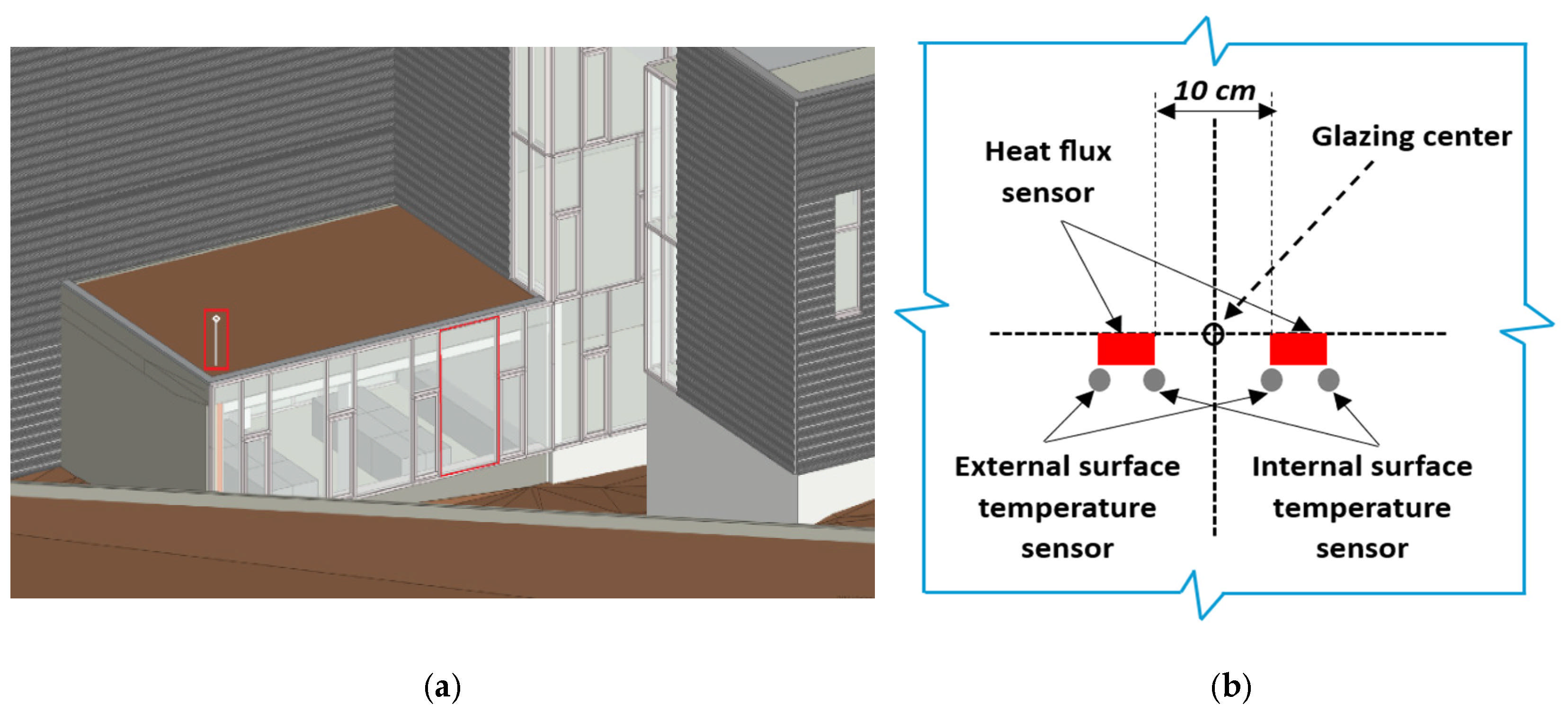
Outdoor environmental conditions were systematically observed and recorded using an all-in-one weather station installed on the office building’s roof (see Figure 2a). Additionally, the indoor ambient temperature and black globe temperature were recorded using multiple K-type thermocouples and a black globe sensor, respectively. These sensors were strategically positioned to avoid direct exposure to solar radiation, thereby minimizing their influence. Only the central part of the glazing is considered in this study. Figure 2b illustrates the measurement setup, which includes two heat flux sensors, two thermocouples for measuring the internal surface temperature, and two for the external surface temperature. Data were logged at 15-min intervals, although the analysis is performed using hourly time steps. Additional details about the measurement equipment can be found in the author’s previous work [35], which serves as the foundation for the current study.

2.4. Machine Learning Approach

As mentioned in the Introduction, this study examines the capability of a machine learning approach to predict two aspects, drawing on experimental data collected during two brief monitoring periods from separate seasons: (1) the dynamic behavior of a relatively large glazing unit in an office building, and (2) daytime thermal comfort in the indoor area near the glazing system. It is important to note that, while the influence of solar radiation on indoor and surface temperatures is accounted for in the thermal comfort analysis (using the black globe sensor data), the impact of direct solar exposure on occupants near the glazing is excluded from this study. Although advanced machine learning methods often achieve strong performance in predictive tasks, this study employs multiple linear regression (MLR) for several reasons. First, the relatively small dataset limits the applicability of more complex models, which generally require larger samples to ensure reliable generalization. Second, MLR provides interpretability, simplicity, and effectiveness in capturing the relationships between multiple input variables and a single output variable, while still delivering reasonable performance in this context [26,27,35].
This study is conducted in three main stages: first, the identification of dependent (target) and independent variables; second, the training and testing of MLR models and the selection of the best-performing models; and third, the comparison of the MLR-predicted results with the actual observed values. A detailed explanation of each stage is provided below.
Stage 1: The identification of dependent (target) and independent variables is one of the most critical steps in any machine learning approach. The dependent variables should reflect key aspects of the study—in this case, the dynamic performance of a glazing unit and indoor thermal comfort. Regarding the independent variables employed in training the MLR models, two main criteria are considered: (1) they must be easily measurable using basic sensors or definable as desired input parameters, and (2) they should exhibit strong linear relationships with the dependent variables. The linear relationships are evaluated using the Pearson correlation coefficient (r). Variables are included in the regression model only if they exhibit a statistically significant correlation, i.e., if r differs significantly from zero [27]. The Pearson coefficient indicates both the strength and direction of a linear relationship, with values ranging from -1 (strong negative correlation) to 1 (strong positive correlation), while a value of 0 indicates no linear correlation.

2.4.1. Dependent and Independent Variables for Dynamic Performance Analysis of the Glazing Unit

As noted in ref. [35], the internal and external surface temperatures of glazing are key indicators of the dynamic performance of a glazing system. These variables reflect how the glazing interacts with both the indoor and outdoor environments. Accordingly, this study selects internal and external surface temperatures of the glazing as the dependent (target) variables. Both daytime and nighttime surface temperature variations are analyzed to capture the glazing system’s response to the presence or absence of solar radiation.
Regarding the independent variables, we adhered to the selection principle stated earlier: only variables that can be measured with basic sensors or specified as needed were considered. This criterion limits the number of eligible input variables. During nighttime periods, the internal and external glazing surface temperatures are predicted from the indoor (office) and outdoor ambient temperatures [35]. In daylight, the feature set is broadened to represent the sun’s influence by incorporating global horizontal radiation and the solar elevation angle—both readily obtainable without specialized instrumentation. Based on findings from the previous study [35], the relative solar azimuth angle did not exhibit a strong linear correlation with glazing surface temperatures and is therefore excluded from the current analysis. Additionally, for both daytime and nighttime scenarios, the potential benefit of including interaction terms (i.e., products of independent variables) is explored in separate model configurations to assess their impact on MLR model performance.

2.4.2. Dependent and Independent Variables for Indoor Thermal Comfort Analysis

In this study, thermal comfort analysis follows Fanger’s comfort indices and the ASHRAE Standard 55-2020 [46,47]. The black globe temperature, measured by a black globe sensor, is selected as the dependent variable, as it is used to determine the mean radiant temperature ( M R T ) and the operative temperature ( T o ). These parameters are essential for calculating the Predicted Mean Vote (PMV) and the Predicted Percentage of Dissatisfied (PPD), which are key indicators of thermal comfort. The relevant calculations are performed using the following equations [48]:
M R T = t g + 273 4 + 0.25 × 10 8 ε t g t a D 0.25 t g t a 0.25 273
T o = M R T + ( t a × 10 v ) 1 + 10 v
In this formulation, t g denotes the black globe temperature (°C), ε represents the emissivity of the globe sensor (dimensionless), D is the black globe sensor diameter (m), t a corresponds to the air temperature (°C), and v indicates the air velocity measured at the height of the black globe sensor ( m · s 1 ). In the case of a standard black globe sensor, the emissivity is 0.95 and the diameter is 0.15 m.
Once the operative temperatures are calculated, the PMV and PPD values can be determined using the CBE Tool [49], which requires four additional input parameters: air velocity ( m · s 1 ), relative humidity (%), metabolic rate (met), and clothing insulation (clo). In this study, since in office environments the metabolic rate of occupants is typically consistent, as individuals are engaged in similar tasks throughout the day, the metabolic rate is fixed at 1.2 met. Clothing insulation is varied according to the specified dates, with values of 0.57 clo for Days 1 and 2 (early October) and 0.74 clo for Days 3 to 6 (late October and early November), in line with recommended values reported in [49]. Relative humidity is maintained at an average of 50% through the use of non-electric dehumidifiers, while the measured air velocity at the area under study does not exceed 0.1 ( m · s 1 ). However, in cases of high air velocity (not observed in this study), it is recommended, according to ref. [50], to follow ISO 7726:2025 [51] for MRT calculation. It is important to note that PPD values below 10% and PMV values within the range of –0.5 to +0.5 are generally considered indicative of acceptable thermal comfort conditions [52].
In this study, a total of eight scenarios with varying sets of independent variables are considered (see Table 1). The simplest scenario, containing the fewest variables, includes only the indoor (office, T i ) and outdoor ( T e ) ambient temperatures. To account for the influence of solar radiation on the indoor environment, the most complex scenario incorporates five main variables along with the interaction terms. These main variables are indoor temperature ( T i ), outdoor temperature ( T e ), global horizontal radiation ( G ), solar elevation angle ( θ s e ), and internal surface temperature of the glazing ( T s i ). The first four variables are supported by the findings in the authors’ previous study [35], while the fifth— T s i —is highlighted as a significant factor affecting thermal comfort in [36]. Evaluating these different scenarios allows for identifying the most critical independent variables necessary for accurate thermal comfort predictions.
Stage 2: At this stage, multiple linear regression (MLR) models are constructed and tested. Once the relevant predictors are identified, the models are developed and their accuracy examined. To validate the approach, this study adopts a holdout strategy in which the dataset is randomly divided: 80% is allocated for model training, while the remaining 20% is reserved for testing. This division enables the model to learn from the majority of the observations while retaining an independent subset to evaluate its performance on unseen data [35,53]. The holdout method is simple yet effective, offering a dependable estimate of generalization ability and helping to limit overfitting without the need for more sophisticated validation schemes.
The dataset is divided into training and testing subsets using the “train_test_split” function from the scikit-learn library in Python 3. The MLR model is then trained on the training data using the fit method, and its performance is evaluated on the test set using the predict method. For the sake of brevity, theoretical details regarding the construction of MLR models and the formula for calculating the Pearson Correlation Coefficient (r) are omitted from this study. These can be found in the author’s previous work [35], which serves as the foundation for the current study. The performance of the trained models is assessed in the testing phase using four statistical indicators: Mean Squared Error (MSE), Root Mean Squared Error (RMSE), Mean Absolute Percentage Error (MAPE), and the Coefficient of Determination (R2). In this context, smaller values of MSE, RMSE, and MAPE signify more accurate predictions, whereas larger R2 values demonstrate stronger explanatory power and better overall model performance.
M S E = 1 n i = 1 n y i y ^ i 2
R M S E = 1 n i = 1 n y i y ^ i 2
M A P E = 1 n i = 1 n y i y ^ i y i × 100
R 2 = i = 1 n ( y i y ^ i ) 2 i = 1 n ( y i Y ¯ ) 2
where Y ¯ is the arithmetic mean of the dependent variable, while n , y i , and y ^ i represent the number of data points, the observed value of the dependent value, and the predicted value of the dependent value, respectively.
At this stage, the best MLR model for each target (dependent) variable—namely, the internal and external surface temperatures of the glazing (for dynamic performance analysis) and the black globe temperature (for thermal comfort analysis)—is selected based on the evaluation metrics. The model with the most favorable evaluation results is chosen to proceed to the next phase, where it is used to predict the target variables for specified periods not included in the dataset used for training the MLR models.
Stage 3: At this stage, the MLR-predicted results for the specified dates are compared with the actual observed values. If the best MLR model selected for thermal comfort prediction corresponds to one of Scenarios 5 to 8, the internal surface temperature of the glazing used in that model is itself predicted by the MLR model developed for that specific variable. In other words, the MLR model used to predict thermal comfort is dependent on the predictions of the MLR model for the internal surface temperature of the glazing.
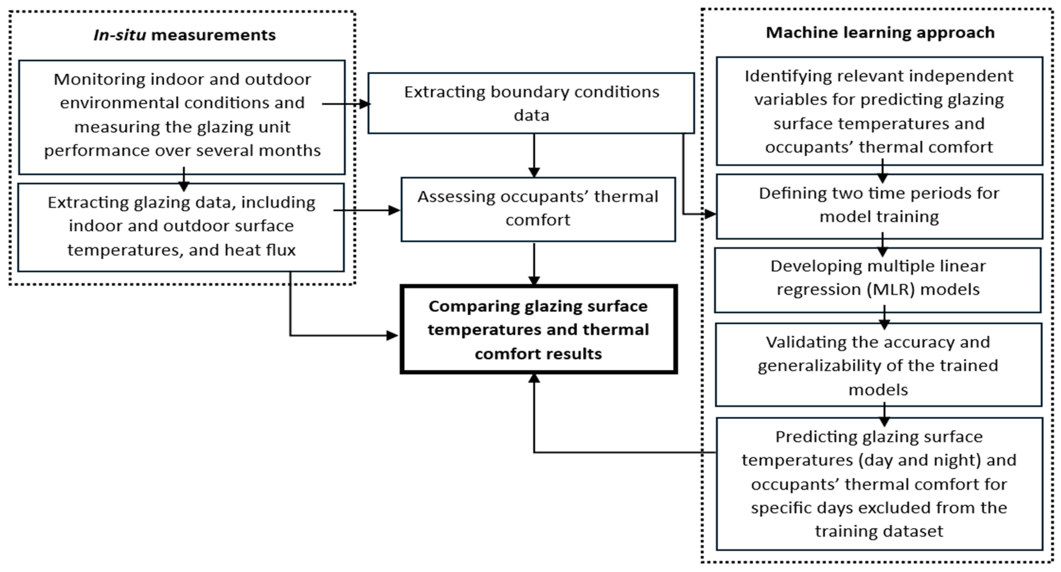
Figure 3 shows the overview of this study.

3. Results

This section is structured around two main criteria: (1) analysis of the glazing’s dynamic behavior using a machine learning approach; and (2) assessment of thermal comfort in the area adjacent to the glazing. In this study, all input variables were retained in their original units without scaling.

3.1. Dynamic Behavior Evaluation

3.1.1. Nighttime Assessment

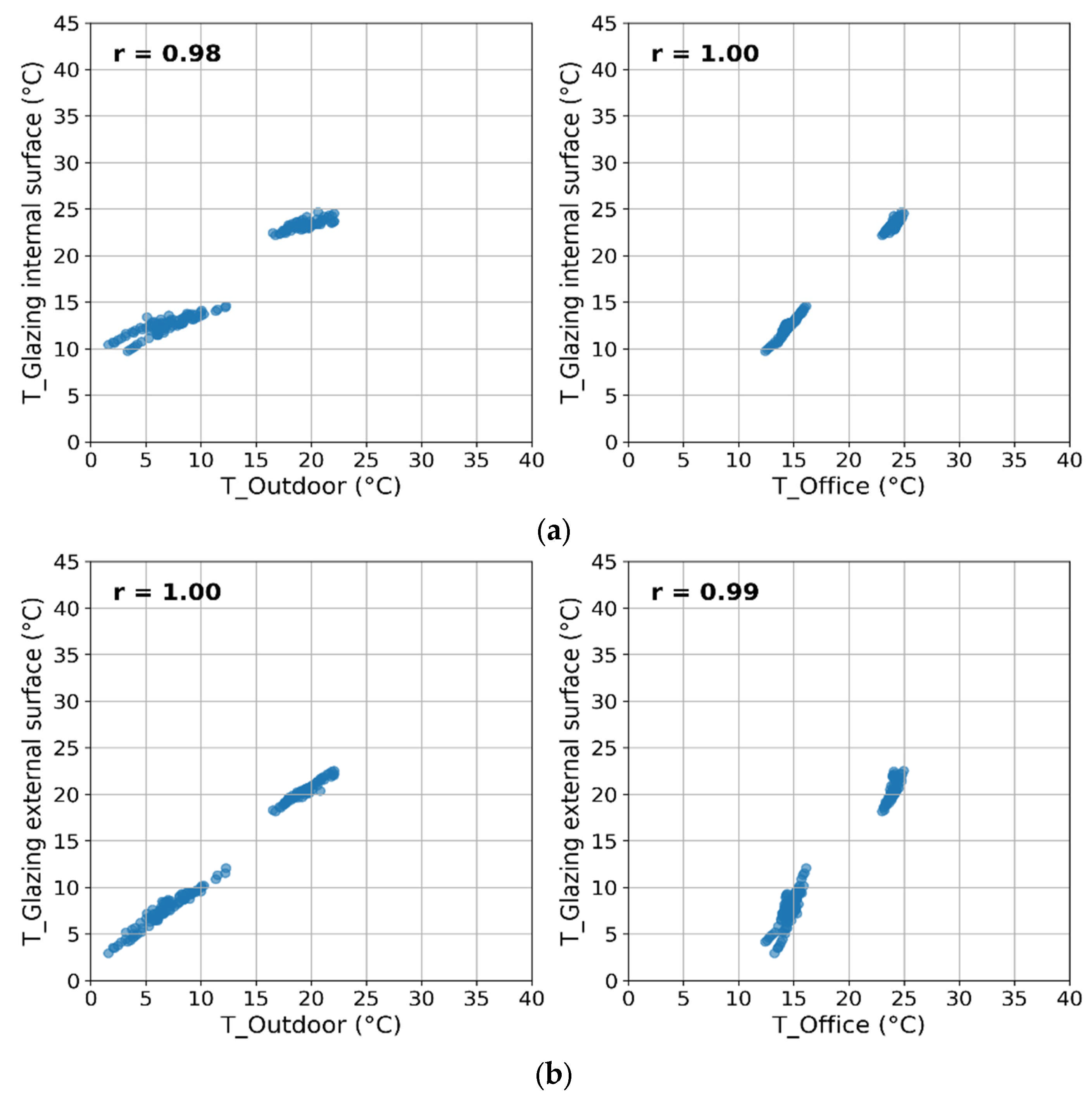
As described in the methodology, indoor (office) and outdoor air temperatures were chosen as predictors for estimating the glazing’s internal and external surface temperatures. These inputs were expected to show strong linear associations with the dependent (target) variables. Figure 4, derived from the nighttime training dataset, demonstrates these associations through the Pearson correlation coefficient (r). The high correlation values confirm the strong linear relationship between the predictors and the glazing surface temperatures, validating the use of indoor and outdoor air temperatures as reliable inputs for the model.
As described in the last section, two multiple linear regression (MLR) models were developed to predict nighttime surface temperatures. In Scenario 1, the model includes only the main independent variables—office and outdoor ambient temperatures. In Scenario 2, interaction terms between the independent variables are included as additional predictors. Table 2 presents the evaluation metrics for both scenarios during the testing (validation) phase. The results indicate that including interaction terms slightly improves the model’s performance for predicting both internal and external surface temperatures. Accordingly, the Scenario 2 MLR models are selected to predict surface temperatures for the specified dates (Nights 1 to 6), which were not part of the training dataset. The selected MLR model equations are as follows:
T s i = 3.786 + 0.167 T e + 1.065 T i 0.004 T e · T i
T s e = 4.116 + 0.740 T e + 0.483 T i 0.003 T e · T i
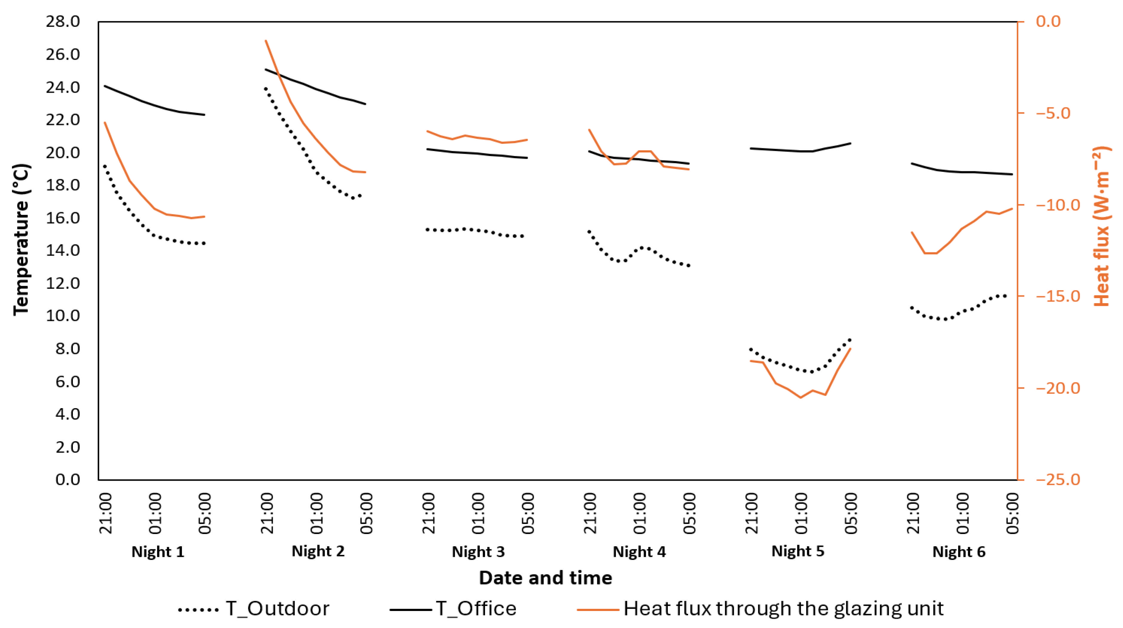
Figure 5 displays the variations in the nighttime ambient temperatures and glazing heat flux for the selected nights from the monitoring periods. As described in the methodology, the evaluation covers three episodes, each comprising two consecutive nights: Nights 1–2 in early October, Nights 3–4 in late October, and Nights 5–6 in early November. The figure shows a progressive decrease in average outdoor temperature across episodes, approaching winter conditions. Additionally, as winter nears, the glazing exhibits a more pronounced dynamic response to outdoor conditions, reflected in increased fluctuations in both ambient temperature and heat flux. These observations underscore the importance of analyzing the glazing’s dynamic behavior.
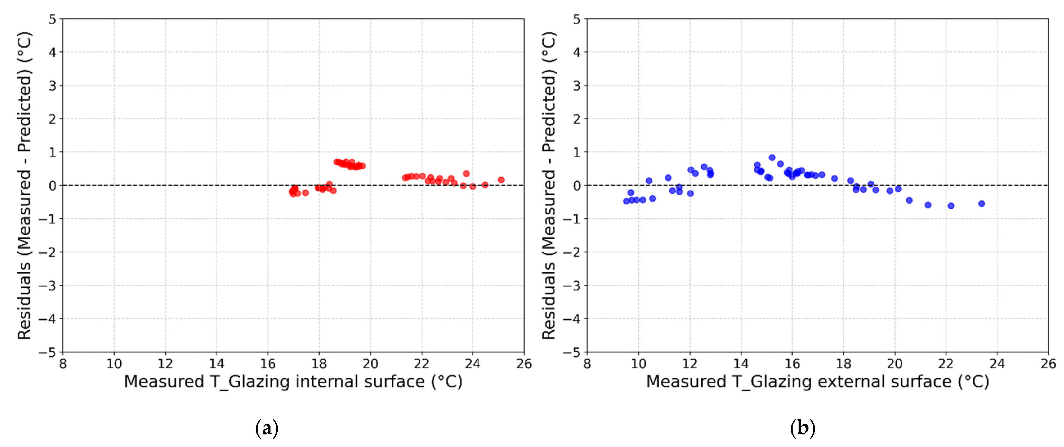
Figure 6 shows that the ML-predicted internal and external surface temperatures closely match the measured values for the specified nights (Night 1 to Night 6), with the maximum deviation not exceeding 1 °C. The corresponding evaluation metrics, presented in Table 3, assess the models’ predictive performance. High R2 values, along with low MAPE, RMSE, and MSE scores, confirm the reliability and accuracy of the trained models under varying outdoor conditions.

3.1.2. Daytime Assessment

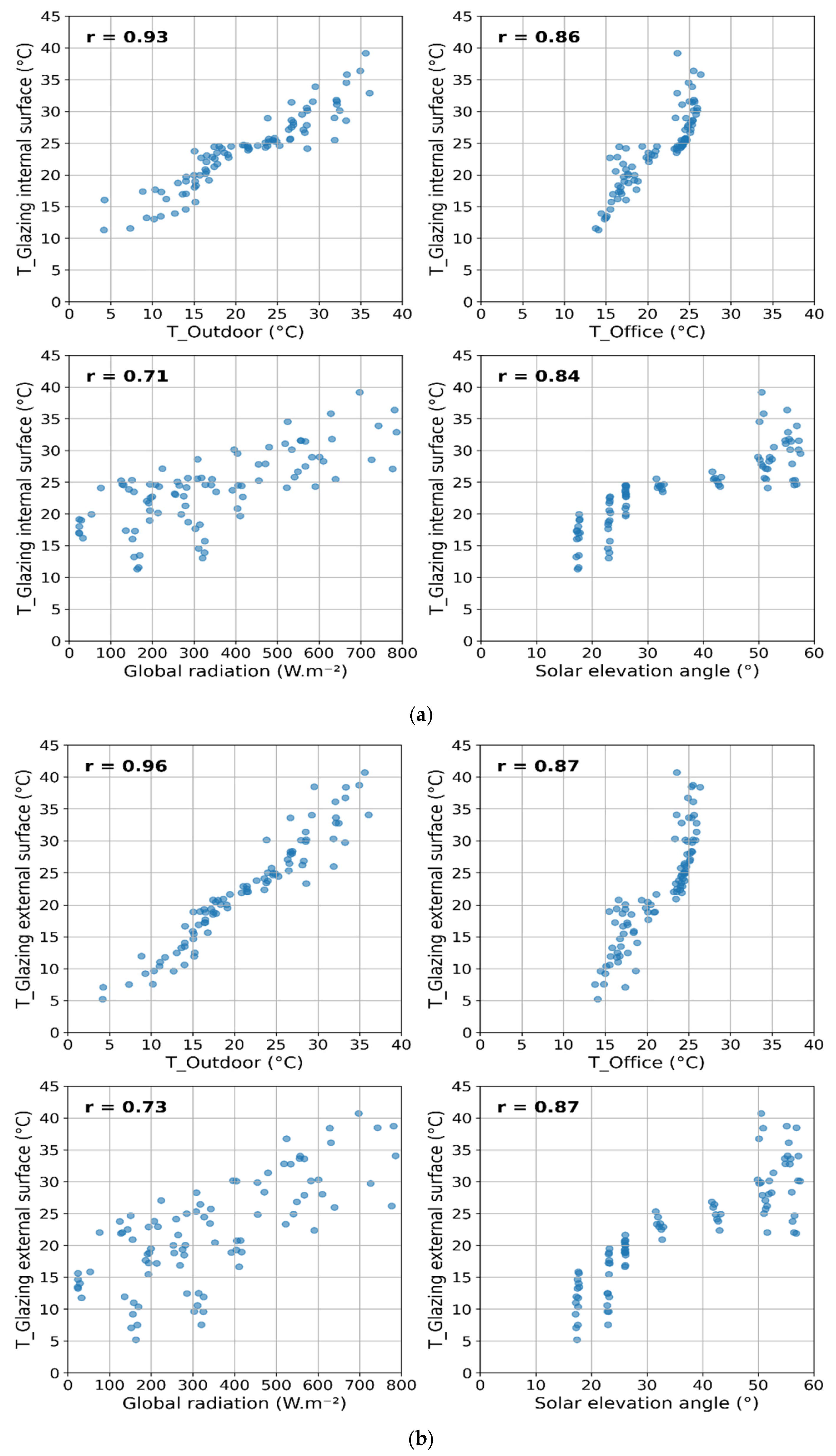
Figure 7, based on the dataset used to train the daytime models, illustrates the linear relationship between the candidate independent variables and the target variables using the Pearson correlation coefficient (r). Although these relationships are not as strong as those observed during nighttime, the r-values remain sufficiently high to justify the selection of these variables for training the daytime MLR models.
Following the same approach as for nighttime modeling, two MLR models were developed to predict daytime surface temperatures. In Scenario 1, the model includes only the primary independent variables: office ambient temperature ( T i ), outdoor ambient temperature ( T e ), global radiation ( G ), and solar elevation angle ( θ s e ). In Scenario 2, interaction terms among the independent variables are also incorporated. Table 4 presents the evaluation metrics from the testing (validation) phase for all models. The inclusion of interaction terms in Scenario 2 improved model performance. For both internal and external surface temperatures, Scenario 2 yields RMSE values below 2 °C, which is considered acceptable [54], and is therefore selected for the next stage. The MLR model equations for Scenario 2, used to predict glazing surface temperatures on the specified dates (Days 1 to 6), are as follows:
T s i = 12.028 + 1.722 T e + 2.033 T i + 0.030 G 1.001 θ s e 0.099 T e · T i + 0.025 T e · θ s e 0.001 T i · G + 0.020 ( T i · θ s e )
T s e = 7.680 + 1.463 T e + 0.999 T i + 0.027 G 0.749 θ s e 0.044 T e · T i + 0.015 T e · θ s e 0.001 T i · G + 0.015 ( T i · θ s e )
Coefficients with absolute values less than 0.001 were excluded from the final regression equation due to their negligible contribution to the model. In both equations, the coefficients show that indoor ( T i ) and outdoor ( T e ) environmental temperatures exert the strongest positive influence on surface temperatures, while global radiation ( G ) has only a minor effect. The interaction terms further indicate that the effect of environmental temperatures is enhanced at higher solar elevation and slightly moderated by global radiation, while the combined rise of indoor and outdoor environmental temperatures reduces their additive impact. These relationships highlight that surface temperatures are governed by both the individual contributions of environmental parameters and their combined effects.
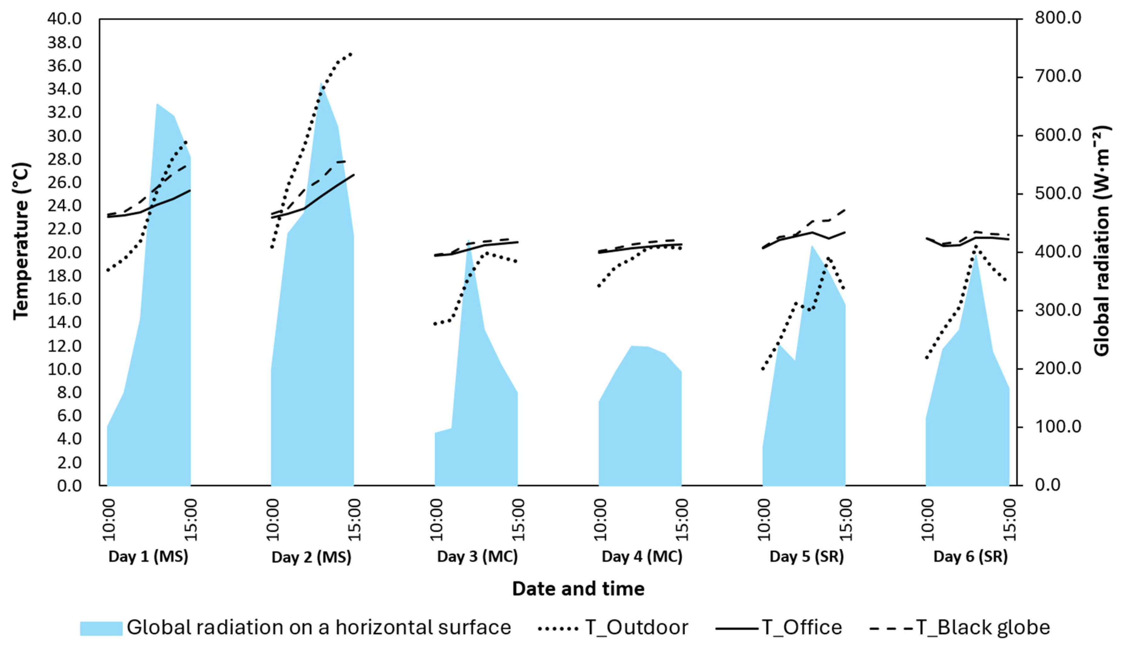
Figure 8 presents daytime measurements of ambient temperatures, black globe temperature, and global radiation on a horizontal surface, recorded between 10:00 and 15:00 for the specified days. These days are grouped into three episodes: Episode 1 (Days 1 and 2) in early October, Episode 2 (Days 3 and 4) in late October, and Episode 3 (Days 5 and 6) in early November. Each episode represents different outdoor conditions: Episode 1 features mostly sunny weather, Episode 2 is predominantly cloudy, and Episode 3 includes both sunny and rainy periods. This selection of varied weather conditions enables a more comprehensive evaluation of the MLR models’ ability to predict the glazing’s dynamic performance. As winter approaches, a decrease in average outdoor temperature is observed. In terms of indoor conditions, Days 1 and 2—with mostly sunny hours—exhibit the highest office and black globe temperatures, while Days 3 and 4—characterized by overcast conditions—show the lowest averages.
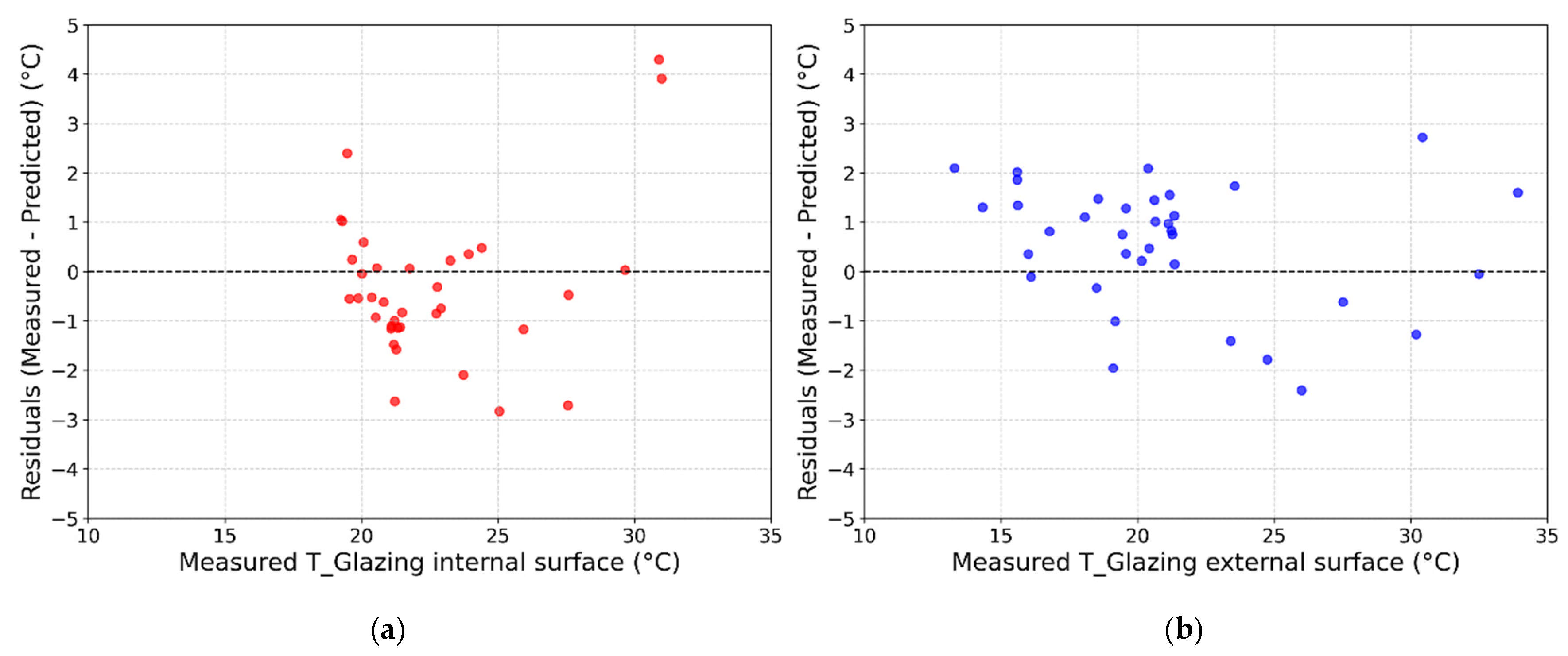
With regard to the prediction of glazing surface temperatures for the specified days (Day 1 to Day 6), Figure 9 shows that daytime predictions are less accurate than nighttime predictions. Nevertheless, the models capture the overall trends of the measured values, with differences exceeding 2 °C only in a few instances. In addition, the largest deviations for both internal and external surface temperatures occur at higher temperature ranges. This discrepancy may be due to the limited representation of such conditions in the training dataset, which may not adequately reflect high-temperature scenarios.
The evaluation metrics assessing the accuracy of the MLR models in predicting the glazing surface temperatures for the specified days are presented in Table 5. The R2 value for the internal surface temperature is lower than that for the external surface temperature; however, both values indicate that the models reasonably explain the variability in the data. A MAPE of 4.90% for the internal surface temperature and 6.35% for the external surface temperature suggests that, on average, the predictions deviate from the actual values by these respective percentages—reflecting relatively low error rates. The RMSE for both internal and external surface temperatures is around 1.50 °C, suggesting that the predicted values generally differ from the measurements by this margin, which remains below the commonly accepted threshold of 2 °C [54]. Importantly, this level of accuracy represents a clear improvement over the findings reported in an earlier study by the same authors [35], particularly for the external surface temperature, where the RMSE is reduced to nearly half of the previous value.

3.2. Thermal Comfort Assessment

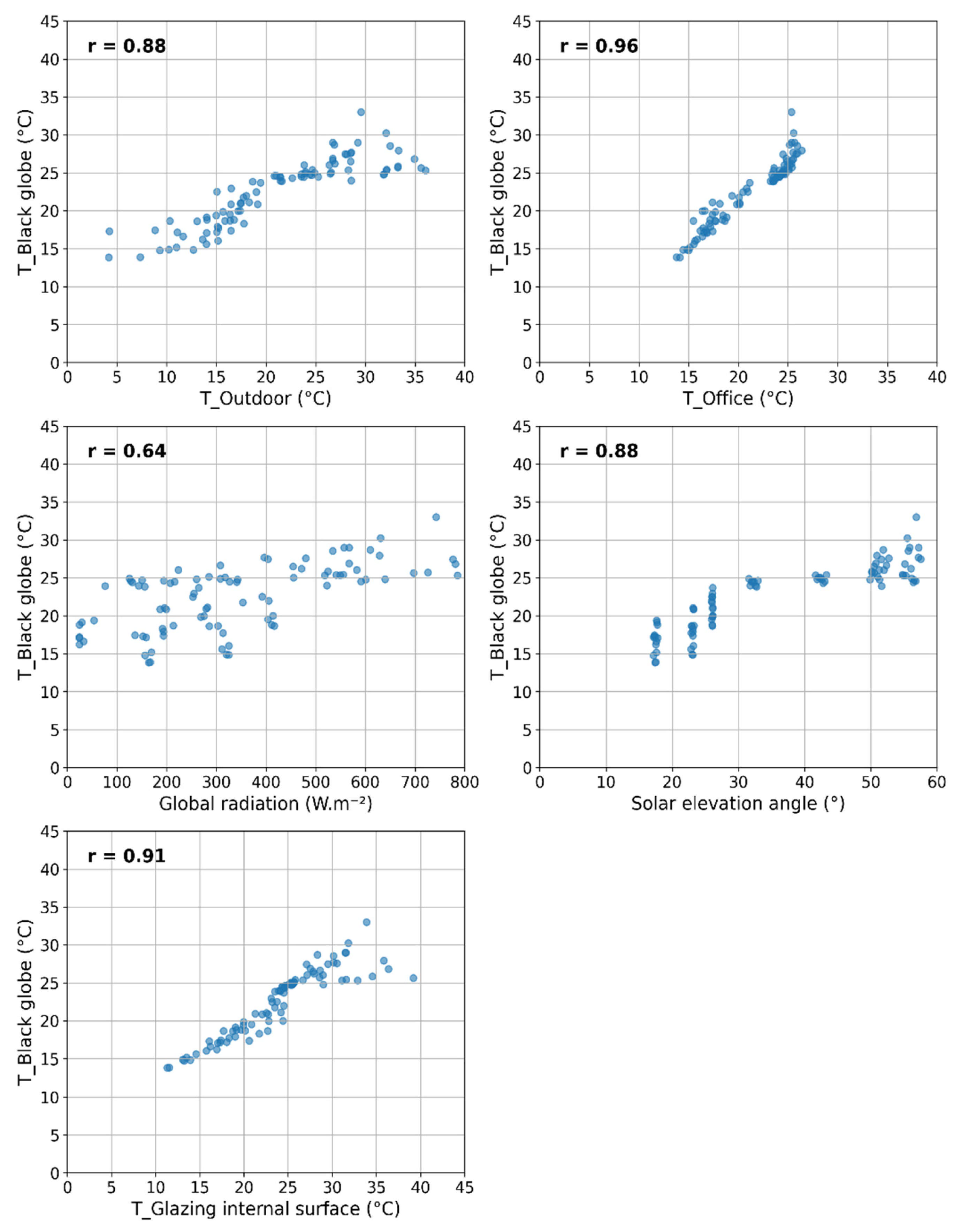
Figure 10, based on the dataset used to train the daytime model for predicting black globe temperature, illustrates the linear relationships between the target variable and the main candidate independent variables: office ambient temperature ( T i ), outdoor ambient temperature ( T e ), global horizontal radiation ( G ), solar elevation angle ( θ s e ), and internal surface temperature of the glazing ( T s i ). While the relationship between global radiation and black globe temperature appears weaker than with the other variables, the corresponding Pearson correlation coefficient (r) still indicates a notable deviation from zero, suggesting a meaningful relationship. As described in the methodology section, multiple scenarios incorporating different combinations of these candidate variables—along with interaction terms—were developed to determine the optimal model. Table 6 presents the evaluation metrics for each scenario during the testing (validation) phase. Scenario 6, which includes the office ambient temperature, outdoor ambient temperature, and the glazing internal surface temperature, along with their interaction terms, demonstrated the best predictive performance. Consequently, this model is selected for the next stage. The equation for the selected MLR model (Scenario 6) is as follows:
t g = 11.101 0.067 T e 0.504 T i + 0.445 T s i + 0.027 T e · T i 0.026 T e · T s i + 0.028 T i · T s i
As outlined in the methodology section, black globe temperature is used to calculate operative temperature (see Equations (1) and (2)), which is then used to determine PMV and PPD values for thermal comfort analysis. Evaluation metrics comparing the predicted and measured black globe and operative temperatures—using the selected MLR model (Scenario 6 or S6)—for Days 1 to 6 (as applied in the daytime glazing dynamic analysis) are presented in Table 7. At this phase, the internal surface temperature of the glazing—required as an independent variable to predict the black globe temperatures—is obtained from the daytime MLR model predictions presented in Section 3.1 for Days 1 to 6. To assess the impact of using the predicted internal surface temperature on the accuracy of black globe and operative temperature predictions in scenario 6, their evaluation metrics are compared with those obtained when the real internal surface temperature (Real T s i ) is used instead. The results, presented in Table 7, show that although the RMSE values for the predicted black globe and operative temperatures remain below 1 °C when the predicted internal surface temperature (predicted T s i ) is used, they are approximately twice as high as those obtained with Real T s i . Furthermore, the R2 values for both predictions increase slightly when Real T s i is used. These findings demonstrate that the accuracy of black globe and operative temperature predictions can be improved by enhancing the accuracy of glazing internal surface temperature predictions.
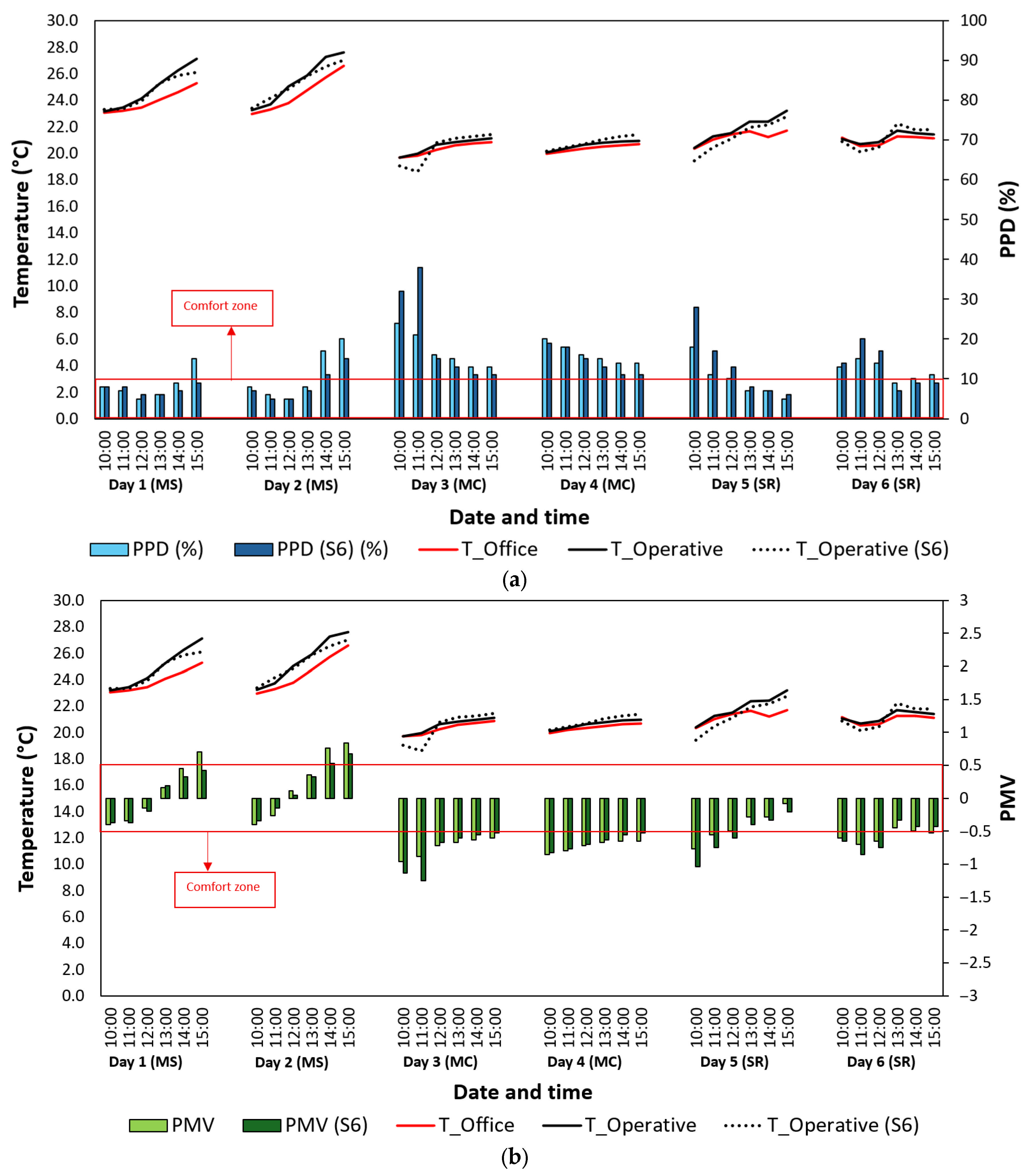
Figure 11 illustrates the differences between the predicted and actual operative temperatures, along with their associated PMV and PPD values. The high R2 and low RMSE values (see Table 7) indicate that the predicted black globe and operative temperatures reasonably align with the measured data for the specified days. As shown in Figure 11, deviations between the predicted and actual PPD and PMV values arise primarily from discrepancies between the predicted and measured black globe temperatures, which subsequently affect operative temperature estimates. The main objective of this study, however, is to evaluate the MLR model’s ability to distinguish between hours of thermal comfort and discomfort. Out of the 36 h analyzed, the MLR model (Scenario 6 or S6) misclassified only three hours, yielding an overall accuracy of approximately 92%. Specifically, during the last hour of Day 1, the actual PPD was 15%, indicating discomfort which the model failed to detect. Likewise, in the final two hours of Day 6, the actual PPD values were 11% and 10% (discomfort), while the model predicted 9% for both—just below the threshold. Although these hours were classified differently, the predicted values were close to the upper limit of the comfort zone, suggesting that the model performs reliably even near classification boundaries.

4. Discussion

In 2024, the European Union adopted a revised version of the Energy Performance of Buildings Directive (EPBD), which mandates that all existing buildings be transformed into zero-emission buildings by 2050 [55,56]. This highlights the importance of in situ methods for obtaining reliable data on the performance of existing building façade elements, including glazing systems [35]. However, long-term in situ testing can be costly, intrusive for occupants, and disruptive. This study investigates the potential of machine learning techniques—specifically, the multiple linear regression (MLR) method—to evaluate the dynamic nighttime and daytime performance of a glazing unit and its impact on the thermal comfort of adjacent spaces using short-term in situ measurements.
For the tested coated double-glazing unit, the MLR models produced nighttime surface temperature estimates that were highly consistent with the experimental measurements. These results suggest that MLR can capture surface temperature dynamics effectively even when trained on relatively limited datasets, such as one week of data collected in September and another in December. These findings align with those of the authors’ previous study [35], in which the MLR models were trained on data collected over two consecutive months (late September to late November). This confirms that combining short-term in situ measurements (two weeks in total—one from a summer period and one from a winter period) with the MLR method enables reliable prediction of nighttime surface temperatures under varying weather conditions.
For daytime glazing surface temperatures, discrepancies between predicted and measured values were observed, particularly during periods with the highest temperatures among the selected days. This may be due to the limited representation of high-temperature conditions in the training dataset. In addition, glazing surface temperatures respond rapidly to solar radiation, making their dynamic behavior more difficult to predict than parameters such as room air temperature, which previous studies have reported with RMSE values below 1 °C [57]. Therefore, it is crucial that training datasets be selected in such a way that they capture the dynamic performance of glazing units, as also recommended in the authors’ earlier work [35]. In the present study, however, compared to [35], daytime surface temperatures were predicted more accurately across a range of weather conditions (sunny, cloudy, rainy, and mixed). As shown in Table 5, the RMSE for both internal and external surface temperatures was approximately 1.5 °C—well within the acceptable range of less than 2 °C [54] and considerably lower than in [35], particularly for external surfaces where the RMSE exceeded 3 °C. These results suggest that training the model with short-term data from two distinct seasons (summer and winter) yields better performance than using a longer dataset spanning two consecutive months with relatively similar weather conditions.
As explained in the methodology section, the use of a train–test approach for MLR model training and performance evaluation with multiple error metrics (MSE, RMSE, MAPE), combined with the decision to keep the models simple by excluding unnecessary predictors, reduces the risk of inflated performance estimates. Furthermore, training the models on two distinct periods (summer and winter weeks) and successfully applying them to predict other periods under varying conditions provides evidence of generalizability and further indicates a lower risk of overfitting.
Regarding thermal comfort, the MLR model predicted periods of thermal discomfort with an overall accuracy of approximately 92%, indicating satisfactory performance consistent with the findings reported in [58]. As shown in Figure 11, the largest deviations between predicted and actual PPD and PMV values occurred when the discrepancy between predicted and actual operative temperatures exceeded 1 °C. This suggests that, to ensure accurate thermal comfort predictions, the difference between predicted and actual operative temperatures should remain below 1 °C. It is important to note that although this study assessed daytime thermal comfort in the area adjacent to glazing using a machine learning approach and accounted for solar radiation through variations in operative temperature, the specific impact of direct solar exposure on occupants positioned very close to the glazing was beyond its scope. This exclusion was due to two reasons: (i) it was first necessary to evaluate the general predictive ability of MLR models for thermal comfort near glazing before addressing more specific effects, and (ii) training MLR models to predict the thermal sensation of occupants exposed to direct solar radiation would require additional independent variables, obtainable only through several supplementary measurement units (e.g., instruments capturing radiation at different heights and distances from the glazing). This requirement necessitates a separate study. Future research may therefore address this limitation.
To better capture the dynamic nature of solar radiation transmitted through glazing and its influence on the indoor environment, future studies should incorporate a greater number of sunny days with high radiation levels in both the in situ measurements and the training datasets for MLR models.
One of the limitations of the present work is that it considers only a single glazing configuration. Expanding the analysis to include different glazing types (e.g., coatings and multi-layer systems), additional orientations, and diverse climatic conditions would enable a more comprehensive assessment of the potential of machine learning as a complementary tool for glazing performance evaluation. To this end, a more holistic measurement strategy is recommended. Laboratory setups such as hot-box chambers and solar simulators could reproduce a wide range of boundary conditions (e.g., temperature gradients, solar radiation intensity, incidence angle, and wind speed), including dynamic patterns such as sinusoidal variations with different amplitudes and periods to represent diverse climates, and would allow systematic testing of a wide range of glazing systems. Crucially, integrating in situ measurement instruments and non-contact methods [56] into the hot-box apparatus would make it possible to monitor glazing performance under these controlled conditions, thereby eliminating the need for multiple costly and time-consuming on-site campaigns across different buildings and glazing systems. In addition, incorporating extra thermocouples and black globe sensors into the measurement setup, positioned at different distances and heights, could further enhance the assessment of solar radiation impacts on occupants’ thermal sensation. The resulting datasets could then be used to train predictive models of glazing performance and comfort, employing not only MLR but also more advanced machine learning methods. Such an approach would help identify the limitations of combining in situ measurements with machine learning techniques, thereby guiding their further development.

5. Conclusions

In efforts to upgrade existing buildings toward nearly zero-energy performance, this study investigated the use of multiple linear regression (MLR) to predict the dynamic performance of glazing systems and their impact on adjacent thermal comfort. Unlike previous studies that relied on longer but seasonally homogeneous datasets, our approach trained models on two short-term, seasonally distinct periods (September and December). This strategy improved the models’ ability to generalize across varied conditions, yielding accurate nighttime predictions and daytime errors of about 1.5 °C RMSE—lower than values reported in prior research. For thermal comfort, the models identified discomfort periods with about 92% accuracy, though deviations increased when operative temperature errors exceeded 1 °C.
The findings demonstrate that training on brief, yet seasonally diverse datasets can enhance prediction accuracy while reducing data collection effort, highlighting the practicality of MLR for building performance assessment. Future work should integrate machine learning with laboratory-based techniques (e.g., hot-box setups, solar simulators, etc.) and in situ measurements, alongside a broader range of glazing samples, to further improve robustness and generalizability.

Author Contributions

Methodology, S.A.M., M.B. and J.P.; Software, S.A.M. and M.B.; Validation, N.S.; Formal analysis, S.A.M.; Investigation, S.A.M.; Data curation, S.A.M.; Writing—original draft, S.A.M.; Writing—review & editing, N.S. and M.G.d.S.; Supervision, N.S., M.B., M.G.d.S. and J.P.; Funding acquisition, N.S. All authors have read and agreed to the published version of the manuscript.

Funding

This research was funded by the Foundation for Science and Technology (FCT Portugal) grant number through funding COMPETE2030-FEDER-00848800.

Data Availability Statement

The original contributions presented in the study are included in the article, further inquiries can be directed to the corresponding author.

Conflicts of Interest

The authors declare no conflict of interest.

Nomenclature

Acronyms t g black globe temperature (°C)
MAPEMean Absolute Percentage Error T e outdoor ambient temperature (°C)
MLMachine Learning T i office ambient temperature (°C)
MLRMultiple Linear Regression T o operative temperature (°C)
MRTMean Radiant Temperature T s e external surface temperature of the glazing (°C)
MSEMean Squared Error T s i internal surface temperature of the glazing (°C)
NZEBsNearly Zero-Energy BuildingsU-valuethermal transmittance ( W · m 2 · K 1 )
PMVPredicted Mean Vote v air velocity at the level of the black globe sensor ( m · s 1 )
PPDPredicted Percentage Dissatisfied y i observed value of the dependent value for the i -th data point
RMSERoot Mean Squared Error y ^ i predicted value of the dependent value for the i -th data point
SHGCSolar Heat Gain Coefficient Y ¯ arithmetic mean of the dependent variable
Abbreviations ε emissivity of the black globe sensor (no dimension)
D diameter of the black globe sensor (m) θ s e solar elevation angle (°)
G global horizontal radiation ( W · m 2 )Subscripts
rPearson Correlation Coefficient i i -th data point ( i = 1 , , n )
R2Coefficient of Determination n total number of data points
t a air temperature (°C)

References

  1. Salazar, S.L.; Yang, R.; Li, D.; Chagolla-Aranda, M.A.; Chávez-Chena, Y.; Simá, E. Advanced hybrid assessment of glazing systems: A comparative analysis using differential and global methods for precise thermal optimization and energy efficiency in building. J. Build. Eng. 2025, 100, 111711. [Google Scholar] [CrossRef]
  2. Moghaddam, S.A.; Simões, N.; da Silva, M.G. Review of the experimental methods for evaluation of windows’ solar heat gain coefficient: From standardized tests to new possibilities. Build. Environ. 2023, 242, 110527. [Google Scholar] [CrossRef]
  3. Wijewardane, S.; Santamouris, M. Smart glazing systems: An industrial outlook. Sol. Compass 2025, 14, 100114. [Google Scholar] [CrossRef]
  4. Mohammadi, M. Keeping it simple: Field testing and techno-economic assessment of a low-cost secondary quad glazing for enhanced energy efficiency in buildings. Energy Built Environ. 2025, in press. [CrossRef]
  5. Teixeira, H.; Rodrigues Moret, A.; Aelenei, D.; Gomes, M.G. Literature review of solar control smart building glazing: Technologies, performance, and research insights. Build. Environ. 2025, 274, 112784. [Google Scholar] [CrossRef]
  6. Song, B.; Yang, L.; Bai, L. Field experimental study of the impact of solar radiation on the thermal comfort of occupants near the glazing area in an office building. Energy Build. 2025, 332, 115422. [Google Scholar] [CrossRef]
  7. Pavlenko, A.M.; Sadko, K. Evaluation of Numerical Methods for Predicting the Energy Performance of Windows. Energies 2022, 16, 1425. [Google Scholar] [CrossRef]
  8. Krarti, M.; Ayari, M.A.; Touati, F.; Paurobally, M.R. Energy Benefits of PV-Integrated Dynamic Overhangs for Residential Buildings in Qatar. Energies 2025, 18, 1156. [Google Scholar] [CrossRef]
  9. Moghaddam, S.A.; Serra, C.; Gameiro Da Silva, M.; Simões, N. Comprehensive Review and Analysis of Glazing Systems towards Nearly Zero-Energy Buildings: Energy Performance, Thermal Comfort, Cost-Effectiveness, and Environmental Impact Perspectives. Energies 2023, 16, 6283. [Google Scholar] [CrossRef]
  10. Shi, Y.; Xi, X.; Zhang, Y.; Xu, H.; Zhang, J.; Zhang, R. Prediction and analysis of the thermal performance of composite vacuum glazing. Energies 2021, 14, 5769. [Google Scholar] [CrossRef]
  11. Peng, J.; Tan, Y.; Fang, Y.; Yang, H.; Song, A.; Curcija, C.; Selkowitz, S. Excellent Insulation Vacuum Glazing for Low-Carbon Buildings: Fabrication, Modeling, and Evaluation. Engineering 2024, in press. [CrossRef]
  12. Pan, Z.; Liu, J.; Wu, H.; Luo, D.; Huang, J. Theoretical-experimental-simulation research on thermal-daylight-electrical performance of PV glazing in high-rise office building in the Greater Bay Area. Appl. Energy 2025, 378, 124739. [Google Scholar] [CrossRef]
  13. Gumbarević, S.; Milovanović, B.; Dalbelo Bašić, B.; Gaši, M. Combining Deep Learning and the Heat Flux Method for In-Situ Thermal-Transmittance Measurement Improvement. Energies 2022, 15, 5029. [Google Scholar] [CrossRef]
  14. Khaled Mohammad, A.; Ghosh, A. Exploring energy consumption for less energy-hungry building in UK using advanced aerogel window. Sol. Energy 2023, 253, 389–400. [Google Scholar] [CrossRef]
  15. Es-sakali, N.; Idrissi Kaitouni, S.; Ait Laasri, I.; Oualid Mghazli, M.; Cherkaoui, M.; Pfafferott, J. Static and dynamic glazing integration for enhanced building efficiency and indoor comfort with thermochromic and electrochromic windows. Therm. Sci. Eng. Prog. 2024, 52, 102681. [Google Scholar] [CrossRef]
  16. Simões, N.; Moghaddam, S.A.; da Silva, M.G. Review of the Experimental Methods for Evaluation of Windows’ Thermal Transmittance: From Standardized Tests to New Possibilities. Buildings 2023, 13, 703. [Google Scholar] [CrossRef]
  17. Kuhn, T.E. State of the art of advanced solar control devices for buildings. Sol. Energy 2017, 154, 112–133. [Google Scholar] [CrossRef]
  18. Ranđelović, D.; Jovanović, V.; Ignjatović, M.; Marchwiński, J.; Kopyłow, O.; Milošević, V. Improving Energy Efficiency of School Buildings: A Case Study of Thermal Insulation and Window Replacement Using Cost-Benefit Analysis and Energy Simulations. Energies 2024, 17, 6176. [Google Scholar] [CrossRef]
  19. Li, X.; Wu, Y. A review of complex window-glazing systems for building energy saving and daylight comfort: Glazing technologies and their building performance prediction. J. Build. Phys. 2024, 48, 496–540. [Google Scholar] [CrossRef]
  20. Guattari, C.; De Cristo, E.; Evangelisti, L.; Gori, P.; Jacoby, R.; Fabiani, C.; Laura, A. Energy & Buildings Thermal characterization of building walls using an equivalent modeling approach. Energy Build. 2025, 329, 115226. [Google Scholar] [CrossRef]
  21. Laukkarinen, A.; Vinha, J. Long-term prediction of hourly indoor air temperature using machine learning. Energy Build. 2024, 325, 114972. [Google Scholar] [CrossRef]
  22. Olu-Ajayi, R.; Alaka, H.; Sulaimon, I.; Sunmola, F.; Ajayi, S. Machine learning for energy performance prediction at the design stage of buildings. Energy Sustain. Dev. 2022, 66, 12–25. [Google Scholar] [CrossRef]
  23. Paschke, F.; Bishara, N.; Schulz, I.; Kocer, C.; Schneider, J.; Maier, A. In situ Ug-value measurement on three different glazing types. J. Phys. Conf. Ser. 2021, 2069, 012134. [Google Scholar] [CrossRef]
  24. Dogan, A.; Kayaci, N.; Bacak, A. Machine learning-based predictive model for temperature and comfort parameters in indoor enviroment using experimantal data. Appl. Therm. Eng. 2025, 259, 124852. [Google Scholar] [CrossRef]
  25. Nardi, I.; Lucchi, E. In Situ Thermal Transmittance Assessment of the Building Envelope: Practical Advice and Outlooks for Standard and Innovative Procedures. Energies 2023, 16, 3319. [Google Scholar] [CrossRef]
  26. Katić, D.; Krstić, H.; Ištoka Otković, I.; Begić Juričić, H. Comparing multiple linear regression and neural network models for predicting heating energy consumption in school buildings in the Federation of Bosnia and Herzegovina. J. Build. Eng. 2024, 97, 110728. [Google Scholar] [CrossRef]
  27. Ciulla, G.; D’Amico, A. Building energy performance forecasting: A multiple linear regression approach. Appl. Energy 2019, 253, 113500. [Google Scholar] [CrossRef]
  28. No, S.T.; Seo, J.S. Analysis of Window Components Affecting U-Value Using Thermal Transmittance Test Results and Multiple Linear Regression Analysis. Adv. Civ. Eng. 2018, 2018, 1780809. [Google Scholar] [CrossRef]
  29. Ibrahim, S.; Kamaruddin, S.A.; Nasir, N.A.N.M. Heating Load of Residential Buildings Using Multiple Linear Regression Artificial Neural Network. J. Adv. Res. Fluid Mech. Therm. Sci. 2022, 92, 28–38. [Google Scholar] [CrossRef]
  30. Troup, L.; Phillips, R.; Eckelman, M.J.; Fannon, D. Effect of window-to-wall ratio on measured energy consumption in US office buildings. Energy Build. 2019, 203, 109434. [Google Scholar] [CrossRef]
  31. Jose, D.M.; Vincent, A.M.; Dwarakish, G.S. Improving multiple model ensemble predictions of daily precipitation and temperature through machine learning techniques. Sci. Rep. 2022, 12, 4678. [Google Scholar] [CrossRef]
  32. Tercha, W.; Tadjer, S.A.; Chekired, F.; Canale, L. Machine Learning-Based Forecasting of Temperature and Solar Irradiance for Photovoltaic Systems. Energies 2024, 17, 1124. [Google Scholar] [CrossRef]
  33. Mutombo, N.M.A.; Numbi, B.P. Development of a Linear Regression Model Based on the Most Influential Predictors for a Research Office Cooling Load. Energies 2022, 15, 5097. [Google Scholar] [CrossRef]
  34. Jiang, T.; Hao, F.; Chen, X.; Zou, Z.; Zheng, S.; Liu, Y.; Xu, S.; Yin, H.; Yang, X. Estimating indoor air temperature by obtaining outdoor building window surface temperature using infrared technology: An exploratory approach. Build. Environ. 2024, 251, 111218. [Google Scholar] [CrossRef] [PubMed]
  35. Moghaddam, S.A.; Brett, M.; da Silva, M.G.; Simões, N. Comprehensive in-situ assessment of glazing systems: Thermal properties, comfort impacts, and machine learning-based predictive modelling. Build. Environ. 2025, 279, 113027. [Google Scholar] [CrossRef]
  36. Song, B.; Bai, L.; Yang, L. The Effects of Exterior Glazing on Human Thermal Comfort in Office Buildings. Energies 2024, 17, 776. [Google Scholar] [CrossRef]
  37. Dogan, T.; Kastner, P.; Mermelstein, R. Surfer: A fast simulation algorithm to predict surface temperatures and mean radiant temperatures in large urban models. Build. Environ. 2021, 196, 107762. [Google Scholar] [CrossRef]
  38. Chereches, M.L.; Chereches, N.C.; Ciobanu, A.A.; Hudisteanu, S.V.; Turcanu, E.F.; Bradu, A.; Popovici, C.G. Experimental study on airflow and temperature predicting in a double skin façade in hot and cold seasons in Romania. Appl. Sci. 2021, 11, 12139. [Google Scholar] [CrossRef]
  39. Long, X.; Jin, Q.; Yu, Z. Multi-objective optimization of PCM-integrated thermochromic glazing to enhance the thermal and daylighting performance. Appl. Therm. Eng. 2025, 266, 125661. [Google Scholar] [CrossRef]
  40. Teixeira, H.; Gomes, M.G.; Moret Rodrigues, A.; Aelenei, D. Solar responsive building glazing: Experimental analysis of the impact of photochromic glazing on indoor thermal and luminous conditions. J. Build. Eng. 2024, 92, 109812. [Google Scholar] [CrossRef]
  41. Duan, Q.; Hinkle, L.; Wang, J.; Zhang, E.; Memari, A. Condensation effects on energy performance of building window systems. Energy Rep. 2021, 7, 7345–7357. [Google Scholar] [CrossRef]
  42. Nguyen, C.K.; Teodosiu, C.; Kuznik, F.; David, D.; Teodosiu, R.; Rusaouën, G. A full-scale experimental study concerning the moisture condensation on building glazing surface. Build. Environ. 2019, 156, 215–224. [Google Scholar] [CrossRef]
  43. Zozulák, M.; Vertaľ, M.; Zozuláková, S.; Dolníková, E.; Katunský, D. Heat-air-moisture modeling for prediction of interior surface condensation of lift-and-slide window—Case study. Heliyon 2023, 9, e15183. [Google Scholar] [CrossRef] [PubMed]
  44. Wang, Y.; Li, X.; Bisby, L. Comparative study of thermal breakage of annealed and tempered glazing with different thicknesses under uniform radiation conditions. Fire Saf. J. 2023, 140, 103867. [Google Scholar] [CrossRef]
  45. ISO 15099; Thermal Performance of Windows, Doors and Shading Devices—Detailed Calculations. International Organization for Standardization: Geneva, Switzerland, 2003.
  46. ASHRAE Standard 55-2020; Thermal Environmental Conditions for Human Occupancy. American Society of Heating, Refrigerating and Air-Conditioning Engineers, Inc.: Atlanta, GA, USA, 2020.
  47. ANSI/ASHRAE Standard 55-2010; Thermal Environmental Conditions for Human Occupancy. American Society of Heating, Refrigerating and Air-Conditioning Engineers, Inc.: Atlanta, GA, USA, 2010.
  48. d’Ambrosio Alfano, F.R.; Dell’isola, M.; Ficco, G.; Palella, B.I.; Riccio, G. On the measurement of the mean radiant temperature by means of globes: An experimental investigation under black enclosure conditions. Build. Environ. 2021, 193, 107655. [Google Scholar] [CrossRef]
  49. Tartarini, F.; Schiavon, S.; Cheung, T.; Hoyt, T. SoftwareX CBE Thermal Comfort Tool: Online tool for thermal comfort calculations and visualizations. SoftwareX 2020, 12, 100563. [Google Scholar] [CrossRef]
  50. Broday, E.E.; Ruivo, C.R.; da Silva, M.G. The use of Monte Carlo method to assess the uncertainty of thermal comfort indices PMV and PPD: Benefits of using a measuring set with an operative temperature probe. J. Build. Eng. 2020, 35, 101961. [Google Scholar] [CrossRef]
  51. ISO 7726:2025; Ergonomics of the Thermal Environment—Instruments for Measuring and Monitoring Physical Quantities. International Organization for Standardization: Geneva, Switzerland, 2025.
  52. Moghaddam, S.A.; Mattsson, M.; Ameen, A.; Akander, J.; da Silva, M.C.G.; Simoes, N. Low-Emissivity Window Films as an Energy Retrofit Option for a Historical Stone Building in Cold Climate. Energies 2021, 14, 7584. [Google Scholar] [CrossRef]
  53. Raschka, S. Model Evaluation, Model Selection, and Algorithm Selection in Machine Learning. University of Wisconsin–Madison, Madison, WI, USA. 2018. Available online: https://arxiv.org/pdf/1811.12808 (accessed on 28 August 2025).
  54. Golosov, N.; Cervone, G. Integrating Thermal Infrared Imaging and Weather Data for Short-Term Prediction of Building Envelope Thermal Appearance. Remote Sens. 2024, 16, 3981. [Google Scholar] [CrossRef]
  55. Hwang, R.; Chiu, H.-C. A Case Study-Based Framework Integrating Simulation, Policy, and Technology for nZEB Retrofits in Taiwan’ s Office Buildings. Energies 2025, 18, 3854. [Google Scholar] [CrossRef]
  56. Evangelisti, L.; De Cristo, E.; Guattari, C.; Gori, P.; De Rubeis, T.; Monteleone, S. Case Studies in Thermal Engineering Preliminary development of a non-contact method for thermal characterization of building walls: Laboratory evaluation. Case Stud. Therm. Eng. 2025, 69, 106012. [Google Scholar] [CrossRef]
  57. Hossein, S.; Besharati, Z.; Abdolrasoul, S. Prediction of room temperature in Trombe solar wall systems using machine learning algorithms. Sustain. Energy Storage 2024, 3, 243–249. [Google Scholar]
  58. Lala, B.; Hagishima, A. A Review of Thermal Comfort in Primary Schools and Future Challenges in Machine Learning Based Prediction for Children. Buildings 2022, 12, 2007. [Google Scholar] [CrossRef]
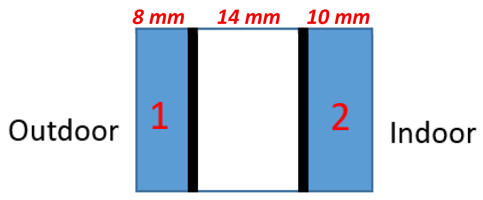
Figure 1. Illustration of the glazing unit with the coating layers highlighted in black.
Energies 18 04656 g001
Figure 2. Illustration of (a) the case study building’s 3D schematic of the ground floor (b) The measurement setup magnified front view focusing on the center of the glazing, showing the positions of the sensors, reproduced from [35]. The south-facing glazing unit under study and the all-in-one weather station placed atop the office, both surrounded by a red rectangle.
Energies 18 04656 g002
Figure 3. Overview of the methodology adopted in this study, adapted from [35].
Energies 18 04656 g003
Figure 4. Visualizations of the correlations between office and outdoor ambient temperatures and (a) internal glazing surface temperature; (b) external glazing surface temperature. The Pearson correlation coefficient (r) indicates the strength of each correlation.
Energies 18 04656 g004
Figure 5. Illustration of nighttime ambient temperature and glazing heat flux patterns for the selected nights from three monitoring periods.
Energies 18 04656 g005
Figure 6. Residuals of measured versus predicted nighttime glazing surface temperatures for the specified nights: (a) internal surface and (b) external surface.
Energies 18 04656 g006
Figure 7. Illustration of the linear relationship between office ambient temperature, outdoor ambient temperature, global radiation on a horizontal surface, and solar elevation angle: (a) internal glazing surface temperature; (b) external glazing surface temperature. The “r” value represents the Pearson correlation coefficient.
Energies 18 04656 g007
Figure 8. Daytime variation of the office and outdoor ambient temperatures, black globe temperature, and global radiation on a horizontal surface. Weather conditions are categorized as follows: (MS) mostly sunny; (MC) mostly cloudy; (SR) sunny and rainy moments.
Energies 18 04656 g008
Figure 9. Residuals of measured versus predicted daytime glazing surface temperatures for the specified dates (Day 1 to Day 6): (a) internal surface and (b) external surface.
Energies 18 04656 g009
Figure 10. Illustration of the linear relationships between black globe temperature and the independent variables: office ambient temperature, outdoor ambient temperature, global horizontal radiation, solar elevation angle, and internal glazing surface temperature.
Energies 18 04656 g010
Figure 11. Illustration of the differences between the predicted (S6) and actual operative temperatures, along with their associated (a) PPD values and (b) PMV values. Weather conditions are categorized as follows: (MS) mostly sunny; (MC) mostly cloudy; (SR) sunny and rainy moments.
Energies 18 04656 g011
Table 1. Candidate independent variables used in the eight scenarios for predicting black globe temperature.
ScenarioIndependent Variables
Scenario 1 T e and T i
Scenario 2 T e , T i , and ( T e · T i )
Scenario 3 T e , T i , G , and θ s e
Scenario 4 T e , T i , G , θ s e , ( T e · T i ), ( T e · G ), ( T i · G ), ( T e · θ s e ), ( T i · θ s e ), and ( G · θ s e )
Scenario 5 T e , T i , and T s i
Scenario 6 T e , T i , T s i , ( T e · T i ), ( T e · T s i ), and ( T i · T s i )
Scenario 7 T e , T i , G , θ s e , and T s i
Scenario 8 T e , T i , G , θ s e , T s i , ( T e · T i ), ( T e · G ), ( T e · θ s e ), ( T e · T s i ), ( T i · G ), ( T i · θ s e ), ( T i · T s i ), ( G · θ s e ), ( G · T s i ), and ( θ s e · T s i )
Table 2. Testing-phase evaluation of MLR models for predicting glazing nighttime surface temperatures.
Dependent VariableScenarioIndependent VariablesMSERMSEMAPER2
T_Glazing internal surfaceScenario 1 T e and T i 0.050.221.130.99
T_Glazing internal surfaceScenario 2 T e , T i , and ( T e · T i )0.040.201.000.99
T_Glazing external surfaceScenario 1 T e and T i 0.150.383.540.99
T_Glazing external surfaceScenario 2 T e , T i , and ( T e · T i )0.140.373.400.99
Table 3. Representation of the evaluation metrics for nighttime MLR-predicted surface temperatures in comparison with measured values for the selected nights.
MSERMSEMAPER2
T_Glazing internal surface (Scenario 2)0.130.361.620.98
T_Glazing external surface (Scenario 2)0.120.342.170.99
Table 4. Testing-phase evaluation of MLR models for predicting glazing daytime surface temperatures.
Dependent VariableScenarioIndependent VariablesMSERMSEMAPER2
T_Glazing internal surfaceScenario 1 T e , T i , G , and θ s e 3.891.977.260.81
T_Glazing internal surfaceScenario 2 T e , T i , G , θ s e , ( T e · T i ), ( T e · G ), ( T i · G ), ( T e · θ s e ), ( T i · θ s e ), and ( G · θ s e )2.901.706.000.86
T_Glazing external surfaceScenario 1 T e , T i , G , and θ s e 5.272.299.730.87
T_Glazing external surfaceScenario 2 T e , T i , G , θ s e , ( T e · T i ), ( T e · G ), ( T i · G ), ( T e · θ s e ), ( T i · θ s e ), and ( G · θ s e )3.661.917.910.91
Table 5. Representation of the evaluation metrics for daytime MLR-predicted surface temperatures in comparison with measured values.
MSERMSEMAPER2
T_Glazing internal surface (Scenario 2)2.381.544.900.78
T_Glazing external surface (Scenario 2)2.121.466.350.91
Table 6. Testing-phase evaluation of MLR models for predicting black globe temperature near the glazing.
ScenarioIndependent VariablesMSERMSEMAPER2
Scenario 1 T e and T i 1.301.144.310.88
Scenario 2 T e , T i , and ( T e · T i )1.181.094.250.89
Scenario 3 T e , T i , G , and θ s e 1.351.164.400.87
Scenario 4 T e , T i , G , θ s e , ( T e · T i ), ( T e · G ), ( T i · G ), ( T e · θ s e ), ( T i · θ s e ), and ( G · θ s e )0.960.983.330.91
Scenario 5 T e , T i , and T s i 0.430.662.290.96
Scenario 6 T e , T i , T s i , ( T e · T i ), ( T e · T s i ), and ( T i · T s i )0.280.531.790.98
Scenario 7 T e , T i , G , θ s e , and T s i 0.470.692.080.96
Scenario 8 T e , T i , G , θ s e , T s i , ( T e · T i ), ( T e · G ), ( T e · θ s e ), ( T e · T s i ), ( T i · G ), ( T i · θ s e ), ( T i · T s i ), ( G · θ s e ), ( G · T s i ), and ( θ s e · T s i )0.300.551.700.97
Table 7. Evaluation metrics for MLR-predicted black globe and operative temperatures (using predicted and real internal surface temperatures) compared with measured values.
MSERMSEMAPER2
Black globe temperature (Predicted T s i )0.400.632.300.93
Black globe temperature (Real T s i )0.110.341.140.98
Operative temperature (Predicted T s i )0.240.491.770.95
Operative   temperature   ( Real   T s i )0.070.260.870.99
Disclaimer/Publisher’s Note: The statements, opinions and data contained in all publications are solely those of the individual author(s) and contributor(s) and not of MDPI and/or the editor(s). MDPI and/or the editor(s) disclaim responsibility for any injury to people or property resulting from any ideas, methods, instructions or products referred to in the content.