A Photovoltaic Power Prediction Framework Based on Multi-Stage Ensemble Learning

Abstract

With the significant increase in solar power generation’s proportion in power systems, the uncertainty of its power output poses increasingly severe challenges to grid operation. In recent years, solar forecasting models have achieved remarkable progress, with various developed models each exhibiting distinct advantages and characteristics. To address complex and variable geographical and meteorological conditions, it is necessary to adopt a multi-model fusion approach to leverage the strengths and adaptability of individual models. This paper proposes a photovoltaic power prediction framework based on multi-stage ensemble learning, which enhances prediction robustness by integrating the complementary advantages of heterogeneous models. The framework employs a three-level optimization architecture: first, a recursive feature elimination (RFE) algorithm based on LightGBM–XGBoost–MLP weighted scoring is used to screen high-discriminative features; second, mutual information and hierarchical clustering are utilized to construct a heterogeneous model pool, enabling competitive intra-group and complementary inter-group model selection; finally, the traditional static weighting strategy is improved by concatenating multi-model prediction results with real-time meteorological data to establish a time-period-based dynamic weight optimization module. The performance of the proposed framework was validated across multiple dimensions—including feature selection, model screening, dynamic integration, and comprehensive performance—using measured data from a 75 MW photovoltaic power plant in Inner Mongolia and the open-source dataset PVOD.

1. Introduction

With the accelerated transformation of the global energy structure, renewable energy represented by solar power generation has been continuously increasing its share in power systems. However, solar power generation is affected by multiple uncertainties, including meteorological conditions, environmental factors, and equipment status, and the randomness and volatility of its power output pose serious challenges to grid dispatch, electricity market trading, and system stability. To address these issues, many scholars have studied methods for solar power generation forecasting [1,2,3].

In recent years, solar power forecasting models have undergone extensive development. Mainstream power forecasting models primarily include physical models [4], statistical models [5], machine learning models, and deep learning models [6,7]. Physical models integrate underlying physical mechanisms such as solar radiation, atmospheric transmission, and photovoltaic cell characteristics to establish mapping relationships between meteorological parameters (e.g., solar radiation) and output power. This approach begins with solar radiation modeling [8], progresses to clear-sky model development [9,10], incorporates atmospheric effects calculations (e.g., Rayleigh scattering, aerosol extinction) [11], and finally performs photovoltaic panel photoelectric conversion calculations [12,13]. Scholars have proposed a physical model based on meteorological parameters and an improved maximum power point tracking (MPPT) algorithm. By predicting meteorological parameters, photovoltaic panel surface radiation, current–voltage characteristics, and executing the MPPT algorithm, hourly photovoltaic power output is forecasted [14]. However, physical models involve complex modeling processes, require high-quality data, and perform poorly under extreme weather conditions. Statistical models, on the other hand, are mostly based on historical power data and meteorological data, employing time-series analysis (e.g., ARIMA and exponential smoothing) [15], regression analysis [16,17], and Kalman filtering [18] to achieve rapid photovoltaic power forecasting. Scholars have evaluated the performance of ARIMA models in solar radiation forecasting under different climatic conditions, and the results show high accuracy in terms of the mean squared error (MSE), root mean squared error (RMSE), and coefficient of determination (R²) [19].

With the rise of machine learning algorithms, methods such as Random Forest [20], XGBoost [21], and Support Vector Regression [22] have been widely applied in the solar energy field by extracting key features to capture nonlinear relationships in data. Machine learning algorithms demonstrate superior advantages in handling complex nonlinear relationships, adaptive capability, and big data mining potential. Scholars have predicted solar irradiance based on meteorological parameters and subsequently forecasted power generation using the predicted irradiance. A comparison of three prediction methods—multiple regression, support vector machine, and neural network—revealed that the neural network model achieved the best accuracy [23]. This feature-based prediction framework combined with shallow networks exhibits strong learning capability for nonlinear weather–power relationships. With recent advancements in computing power, deep learning approaches employing Recurrent Neural Network (RNN) [24], Gated Recurrent Unit (GRU) [25], and Long Short-Term Memory (LSTM) [26] for time-series forecasting have further enhanced model learning capability. Based on three years of data from an Australian photovoltaic power station, a study combining LSTM and TCN models demonstrated high accuracy in both single-step and multi-step power prediction, effectively extracting features, capturing information, and learning data patterns [27]. The latest research trends indicate that Transformer architectures based on attention mechanisms show advantages in long-sequence dependency modeling. Research focused on day-ahead photovoltaic power forecasting using Transformer variants demonstrated significant advantages in RMSE metrics and competitive performance across different datasets and prediction horizons [28]. Scholars proposed PVTransNet, a multi-step photovoltaic power forecasting model based on Transformer networks, which significantly improves prediction accuracy by integrating historical PV generation data, meteorological observations, weather forecasts, and solar geometry data [29].

These prediction methods primarily rely on single models while neglecting the complementarity between different models, with their performance being constrained by the inherent limitations of each model. For instance, physical models are highly sensitive to the accuracy of meteorological parameters, while statistical models struggle to capture complex nonlinear relationships. As for machine learning and deep learning models, their performance varies significantly when applied to different power plants with complex operating conditions due to variations in meteorological factors and data quality. To address these limitations, researchers have investigated ensemble learning-based prediction models. For example, one study proposed a hybrid deep learning framework for photovoltaic power forecasting that combines Maximum Overlap Discrete Wavelet Transform (MODWT) with Long Short-Term Memory (LSTM) networks, aggregating predictions from multiple LSTM models using a weighted averaging method [30]. Another study explored four different ensemble methods: simple averaging, linear weighted averaging, nonlinear weighted averaging, and inverse variance-based combination. The results demonstrated that the inverse variance-based combination method generally performs best, improving the accuracy of day-ahead predictions by 4.55–36.21% [31].

Ensemble learning-based forecasting frameworks can enhance accuracy through integration strategies; yet, these methods typically focus only on simple or weighted averaging of model outputs. They still rely on single models for feature selection and lack systematic screening criteria for sub-model pool selection, failing to consider the impact of model diversity on prediction accuracy. For result integration, they employ either simple averaging or static weighting, without accounting for temporal dimensions or proper model weighting under different weather conditions.

To address these limitations, this paper proposes a multi-stage ensemble learning framework that optimizes three key aspects: feature selection, model screening, and dynamic result integration. Scholars have utilized open data and machine learning algorithms to predict short-term (hourly) power generation at newly operational photovoltaic power plants, emphasizing the importance of multi-location evaluation [32]. Accordingly, the proposed method was tested at multiple sites within public datasets and at a real-world 75 MW power station in Inner Mongolia. Experimental results demonstrate that the proposed method outperforms baseline models across multiple sites.

The highlights of this paper are as follows:

• At the feature selection level, a multi-model-weighted RFE-based evaluation method is proposed, which effectively enhances the discriminative power and robustness of input features by leveraging complementary advantages.
• At the model construction level, an adaptive screening mechanism based on mutual information and hierarchical clustering is introduced to build a heterogeneous model pool, achieving intra-group competition and inter-group complementarity, thereby enhancing model diversity and generalization capability.
• At the ensemble strategy level, traditional static weighting methods are improved by integrating multi-model outputs and real-time meteorological data to construct a time-dependent dynamic weight optimization module, boosting prediction accuracy across different time steps and weather conditions.

The performance of the proposed forecasting framework was validated across four dimensions—feature selection, model screening, ensemble strategy, and comprehensive performance—using data from a 75 MW power plant and the open-source PVOD dataset.

2. Data and Method

2.1. Data

The data used in this study consist of two parts: one based on the open-source dataset PVOD [33] and the other from a 75 MW power station located on the Inner Mongolia Plateau.

The open-source PVOD dataset includes ground monitoring data (such as temperature, humidity, irradiance, etc.) and numerical weather prediction data (global radiation, direct radiation, temperature, etc.) from 10 photovoltaic power stations. The temporal resolution of the data is 15 min. The dataset is divided into 80% for training and 20% for testing.

The mentioned 75 MW real power station on the Inner Mongolia Plateau is located at 41.98° N latitude and 111.39° E longitude. The dataset comprises both ground-based meteorological station measurements and numerical weather prediction (NWP) data, including wind speed, wind direction, temperature, atmospheric pressure, humidity, irradiance, as well as predicted cloud cover from NWP. The time span covers from September 2022 to September 2024, with a temporal resolution of 15 min.

The first year’s data (1 September 2022–31 August 2023) were used for model development, while the second year’s data served for testing operational performance. Within the first-year data, an 80–20 split was implemented, with 80% allocated for training and 20% for validation purposes.

2.2. Method

The proposed prediction framework consists of five components: data preprocessing, feature selection, model selection, first-level training network, and second-level fusion network. The overall workflow framework is illustrated in Figure 1.

2.2.1. Data Preprocessing

The raw data are transformed into model-ready features through data cleaning and feature engineering to enhance data quality and prediction model performance. Data cleaning primarily involves handling missing values and removing outliers. A hybrid approach combining physical rules and statistical tests is employed to detect outliers. In terms of physical rule filtering, power values that fall outside the theoretical output range of photovoltaic modules are eliminated, such as power values during nighttime with non-zero irradiance or data exceeding the installed capacity on sunny days. For statistical testing, the dataset is divided monthly, and the mean and standard deviation of each meteorological variable and power output at a 15 min temporal resolution are calculated. A dynamic threshold interval is established based on the 3σ criterion to identify statistically significant outliers. During the outlier handling phase, differentiated strategies are applied for different types of anomalous patterns. For centralized anomalies caused by factors like weather station communication failures, which manifest as overall abnormal data for a day or consecutive days, a bulk removal strategy is adopted, eliminating all observed data within the relevant dates from the training set. For discretely occurring individual outliers, a spatiotemporal proximity replacement method is used, where normal observed values from the same time on adjacent dates are selected for substitution based on meteorological similarity principles. Feature engineering includes constructing interaction features (e.g., squared or product terms) from basic features, as well as calculating solar elevation and azimuth angles using high-precision astronomical algorithms.

2.2.2. Feature Selector

This study constructs an initial feature set based on actual power plant operation data, primarily including meteorological features (covering temperature, humidity, wind speed, wind direction, air pressure, and solar radiation), power features, and temporal features. To screen the most valuable features for the prediction task from the raw data while reducing the negative impact of redundant and irrelevant features on model performance and improving the model’s generalization capability, this study employs the Recursive Feature Elimination (RFE) algorithm for feature selection.

RFE is a wrapper-based feature selection method that relies on model performance, with its core idea being to recursively build models and eliminate the least important features to obtain the optimal feature subset. The algorithm implementation process is shown in Figure 2. The complete feature set is utilized to independently train LightGBM, XGBoost, and MLP models. Model performance is evaluated using 3-fold cross-validation, with the negative mean squared error as the metric. Adaptive weights are assigned proportionally to the reciprocal of each model’s mean squared error (weight = 1/MSE), followed by L1-normalization across all models to obtain final weighting coefficients. By ranking feature importance, the least important features are eliminated, and the remaining features continue to be used with the three models to obtain new weighted performance scores. This iterative cycle continues until the weighted performance scores no longer improve, thereby outputting the optimal subset. A preset threshold permits moderate fluctuations in the weighted score as the number of features decreases. When a significant decline in the weighted score is observed, the critical point is identified as the optimal performance point. This method achieves efficient and robust feature selection by combining multi-model weighted feature importance evaluation with dynamically terminated recursive feature elimination. The adoption of weighted voting from three base models avoids the evaluation bias of single models and achieves complementary advantages.

2.2.3. Model Selector

Existing research on power prediction primarily focuses on three core aspects: feature selection, model construction, and hyperparameter optimization. Among these, model construction methods have reached a relatively mature stage. However, the literature review reveals significant limitations in current model selection strategies: on one hand, the model selection process often exhibits randomness and blindness, lacking systematic criteria; on the other hand, while different models possess specific applicable domains, existing methods fail to establish model selection standards that match data characteristics.

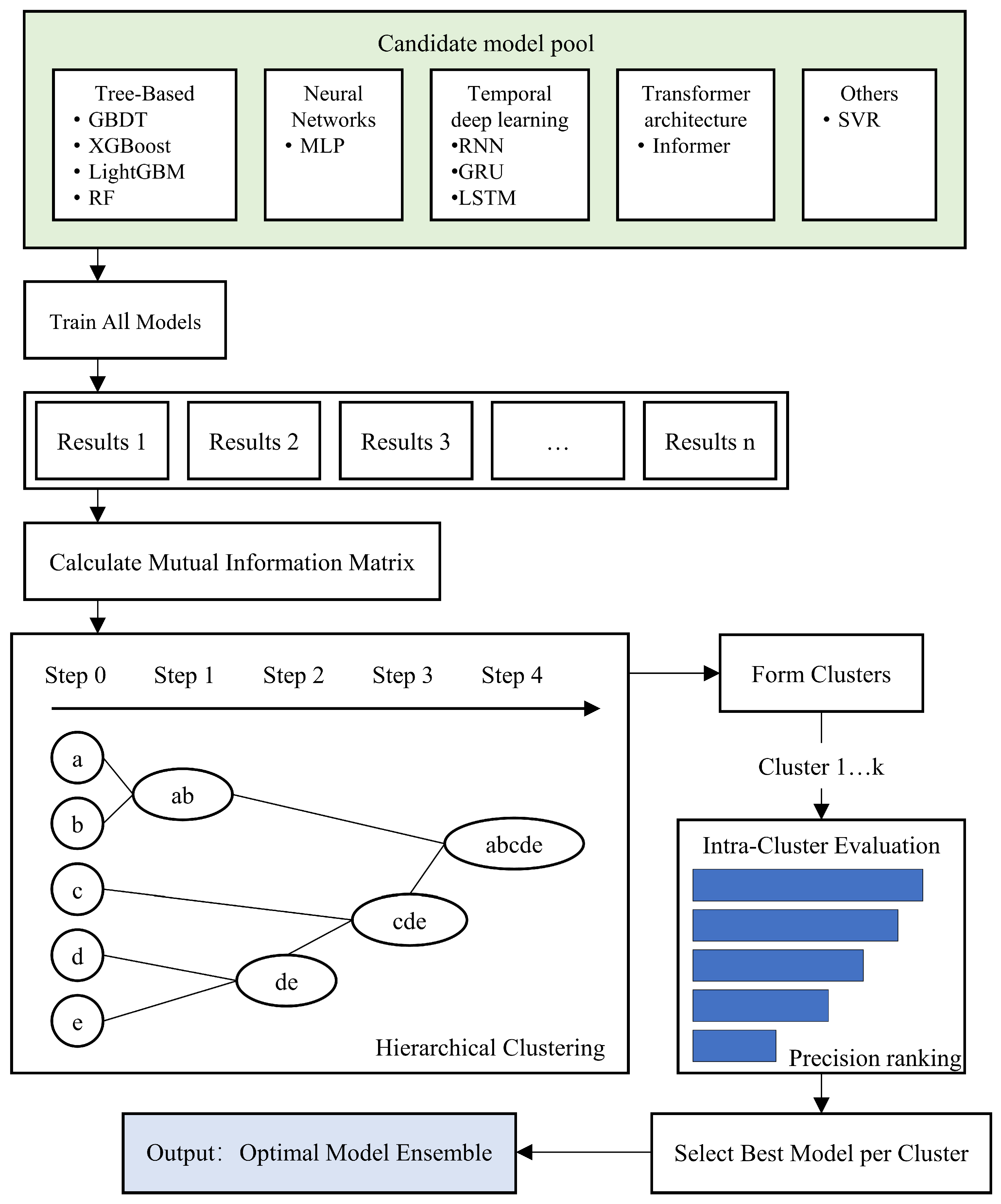
To address this, this study proposes a hierarchical clustering-based adaptive model selection framework, as shown in Figure 3, aiming to fully explore model diversity. Its core design principles encompass two dimensions: (1) diversity assurance—ensuring the model ensemble covers diverse prediction characteristics through cluster analysis; (2) difference optimization—selecting model combinations with significant complementarity.

The specific implementation path is as follows: first, construct a candidate model pool containing mainstream machine learning algorithms, such as tree-based models (Gradient-Boosting Decision Tree (GBDT), XGBoost, LightGBM, Random Forest), traditional neural networks (MLP), time-series deep learning networks (RNN, GRU, LSTM), and transformer-based models (Informer). Train all candidate models, then perform hierarchical clustering based on prediction results to generate a dendrogram division of models. The similarity metric is calculated using mutual information between model prediction results. After iterative convergence, the algorithm automatically generates several model clusters, where models within each cluster exhibit highly similar prediction behaviors. By evaluating performance metrics like Root Mean Square Error (RMSE) for models within each cluster and ranking them by accuracy, the best-performing representative model from each cluster is selected, ultimately constructing an optimal model ensemble that combines both diversity and difference.

The proposed mutual information is a metric in information theory that quantifies the dependency between two variables. Given model predictions X and Y, the mutual information is expressed as:

$$I\left(X,Y\right)={\displaystyle \sum _{y\in Y}{\displaystyle \sum _{x\in X}p\left(x,y\right)\log \frac{p\left(x,y\right)}{p\left(x\right)p\left(y\right)}}}$$

(1)

Higher mutual information values indicate more similar prediction behaviors.

For multiple models M₁, M₂, …, Mₙ, the mutual information between any pair of model outputs Pᵢ and Pⱼ is computed. A non-parametric estimation method based on k-nearest neighbors is employed. This approach leverages the local density of sample points in the joint space and marginal spaces to estimate mutual information, thereby circumventing the need for explicit probability density function fitting. For models Mᵢ and Mⱼ, the mutual information is calculated as follows:

$$M{I}_{ij}={\displaystyle \frac{1}{T}}{\displaystyle \sum _{t=1}^{T}I\left(P_i^t,P_j^t\right)}$$

(2)

A symmetric mutual information matrix MI is constructed. The diagonal elements represent the mutual information between each model and itself.

To satisfy the distance metric requirement for hierarchical clustering, the mutual information similarity measure is converted into a distance metric using the following transformation. The distance between models Mᵢ and Mⱼ is defined as:

$$D_{ij}=1-{\displaystyle \frac{M{I}_{ij}-\min \left(MI\right)}{\max \left(MI\right)-\min \left(MI\right)}}$$

(3)

A smaller distance value indicates greater similarity in the predictive behavior between models. The distance values on the main diagonal are zero.

Based on this, a hierarchical clustering method is employed to cluster the candidate models. To ensure minimal intra-cluster divergence and maximal inter-cluster divergence, the number of clusters is determined using the elbow method. The within-cluster sum of squares is computed for different numbers of clusters, and the elbow point in the curve of within-cluster sum of squares versus the number of clusters is identified to determine the optimal number of clusters.

After completing the cluster partitioning, a representative model selection mechanism is proposed to avoid retaining excessive redundant models within the same cluster. For each cluster, the prediction error between each model’s output and the true labels is computed, and the model with the smallest error within the cluster is selected as the representative model.

2.2.4. First-Level Training Network

This section details the construction process of the first-level prediction models. This layer performs parallel training on multiple heterogeneous models, with distinct prediction characteristics selected through hierarchical clustering, generating initial prediction results. These predicted values form an intermediate feature space and serve as input for the second-level meta-learner to further optimize predictions.

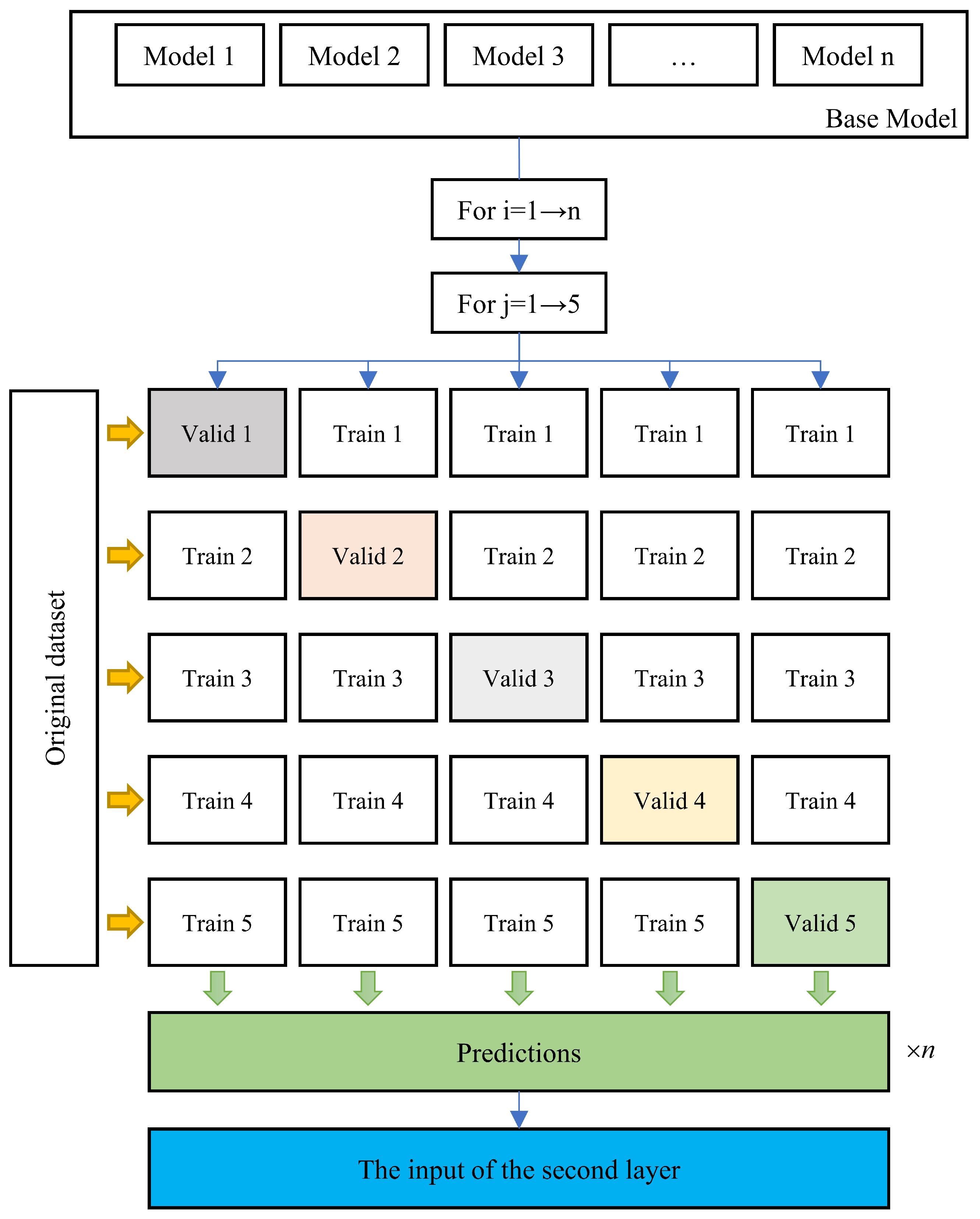
For training the multiple heterogeneous models in the first layer, we employ a k-fold cross-validation approach (5-fold in this study) instead of direct training on the entire training set. The primary motivations for this approach are:

• Preventing data leakage. If models are trained directly on the complete training set and predict the same data, their predictions become highly correlated with true labels. Since base learners have already seen the data, the meta-learner would learn the “false” fitting capability rather than genuine generalization ability, ultimately compromising Stacking performance. K-fold cross-validation separates training and validation data, ensuring base models predict unseen samples for unbiased estimation.
• Improving data utilization. In k-fold cross-validation, the training set is divided into k mutually exclusive subsets (folds). Each subset serves as the validation set in turn, while the remaining k − 1 subsets are used for training. Thus, every sample participates in both training (k − 1 times) and validation (once), maximizing data usage and avoiding sample loss from fixed validation splits.
• Reducing overfitting risk. As base models train on k different training subsets and predict on independent validation sets, their output predictions better reflect generalization capability rather than memorization of training data. Through multiple (k) training–validation cycles, model evaluation becomes more stable and accurate for unseen data prediction, both decreasing the overfitting risk and enhancing the ensemble model’s final generalization performance.

Each base model undergoes 5-fold cross-validation training, as shown in Figure 4. After reserving the final test set, sequence modeling is performed on the remaining training period data (assumed to be n time points). The power values for the next 16 time steps are predicted based on the features of the past 16 time steps. The constructed feature matrix X has a dimension of (n − 16 × 2 + 1, num_features, 16), and the label vector y has a dimension of (n − 16 × 2 + 1, 16). Each sample i represents a time window. X[i] contains num_features features from time point i to i + 15. y[i] contains 16 power values from time point i + 16 to i + 31. Sliding-window cross-validation is adopted, strictly ensuring that validation samples (future data) always come after training samples (historical data) to prevent data leakage. The specific procedure is as follows:

• The complete sample set, arranged in chronological order, is divided into 5 consecutive time segments.
• For subset i, a portion at the end is used as the validation set, and all preceding segments are used as the training set.
• The model is trained on the current training set and used to predict on the validation set, yielding predictions for that segment.
• Steps 2 and 3 are repeated until all 5 segments are traversed, and the predictions from each validation set are concatenated to form the complete output.
• Performance metrics are calculated for each validation fold, and the average performance across the 5 folds is used as the evaluation of the model’s generalization capability.

After 5 training iterations, model performance becomes more robust, as testing occurs across different data partitions, avoiding over-reliance on any specific split.

The loss function for multiple models aligns with the local grid’s ultra-short-term forecasting standards, defined as:

$$Loss=(1-{\displaystyle \frac{\sqrt{{\displaystyle \sum _{j=1}^{16}\left[{\left(p_j-p_j^{\prime }\right)}^2\frac{\left|p_j-p_j^{\prime }\right|}{{\displaystyle \sum _{j=1}^{16}\left|p_j-p_j^{\prime }\right|}}\right]}}}{Cap}})\times 100\%$$

(4)

where $Cap$ represents installed capacity, and $p_j$ and $p_j^{\prime }$ denote predicted and actual power, respectively. This loss function assigns different weights to 16 prediction values, proving stricter than RMSE by imposing higher technical demands. Typically, prediction accuracy degrades with longer time intervals. While RMSE averages errors across 16 timesteps, this metric penalizes larger errors more severely.

2.2.5. Feature Enhancement: Secondary Feature Construction

In ensemble learning frameworks, traditional meta-learning typically relies solely on the predictions of base models for static weighting or linear combination, neglecting the impact of crucial dynamic features from the original data on model performance. To enhance the adaptability and robustness of the ensemble model, this workflow introduces a feature enhancement module prior to meta-learning, designed to dynamically adjust the weights of different base models for better adaptation to temporal variations and external environmental factors (e.g., weather conditions). The feature enhancement module incorporates weather conditions from the original data as auxiliary input for meta-learning, while also accounting for temporal dimension effects. These two feature types exert significant influence in power forecasting. Weather factors directly affect prediction targets, necessitating dynamic weight adjustments in meta-learning based on current conditions. Different base models demonstrate varying performance across prediction time steps—some may excel at near-term predictions, while others perform better for longer time horizons.

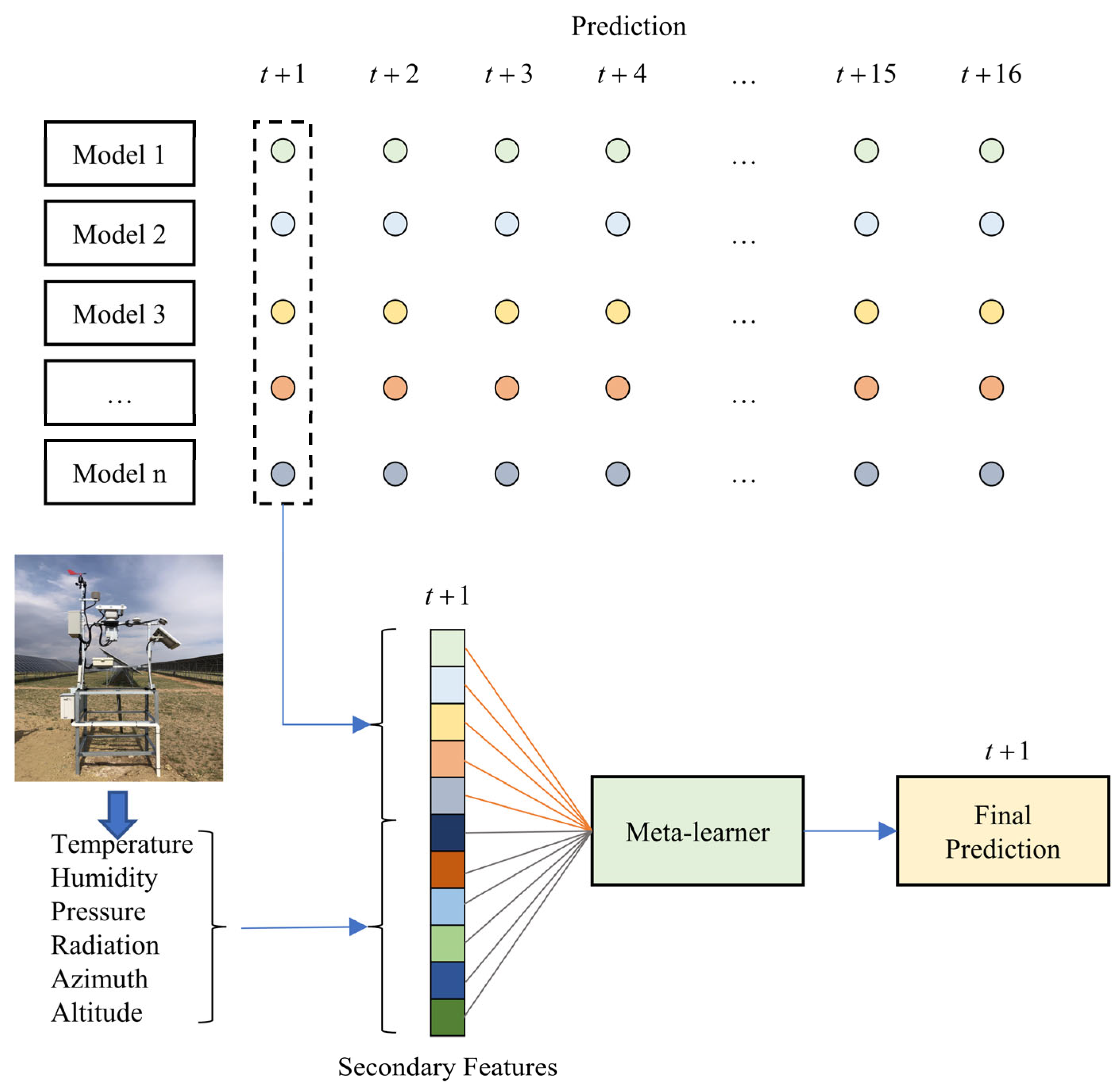
The proposed method fully utilizes original meteorological data by fusing parallel predictions from multiple models with initial raw data to construct secondary features for second-stage model optimization, as illustrated in Figure 5. Aligned with local grid standards for ultra-short-term forecasting, the solar power prediction requires 16 output values (4 h horizon at 15 min resolution). For each individual time step among these 16, predictions from multiple parallel models are concatenated with original meteorological data to serve as the input for secondary fusion learning, enabling the model to learn optimal decision strategies for different base models under varying weather conditions. This approach not only preserves the physical significance of original meteorological variables but also mitigates overfitting risks from individual models through the integration of multi-model predictions.

2.2.6. Second-Level Fusion Learning

The second layer of the proposed framework primarily learns from the predictions of first-layer base models to leverage their respective strengths and achieve superior performance compared to any single model. Since the first-layer network has already captured most mapping relationships between features and predictions, the fusion learner in this layer selects a model with strong expressive power but low overfitting risk. Accordingly, this layer employs Support Vector Regression (SVR) as the fusion learner instead of deep network structures.

To address the sequential characteristics of predictions, we propose a time-segmented recursive optimization method. By combining multi-model prediction fusion with enhanced original meteorological features, we construct a high-information-density input space. The SVR’s capability in modeling complex nonlinear relationships enables secondary optimization for final predictions. Using these enhanced secondary features as input to the SVR decision optimization system, we build 16 independent optimization models for the 16 time steps of each prediction, as shown in Figure 6. The objective function is defined as:

$$\underset{w,b}{\min }{\displaystyle \frac{1}{2}}{‖w‖}^2+C{\displaystyle \sum _{i=1}^n\left({\xi }_i+{\xi }_i^{*}\right)}$$

(5)

where, for each sample $\left(x_i,y_i\right)$, the constraint conditions are:

$$y_i-\left(w^T{x}_i+b\right)\le \epsilon +{\xi }_i^{*}$$

(6)

$$\left(w^T{x}_i+b\right)-y_i\le \epsilon +{\xi }_i$$

(7)

$${\xi }_i,{\xi }_i^{*}\ge 0$$

(8)

where ${\xi }_i$ and ${\xi }_i^{*}$ are slack variables used to handle samples with errors exceeding $\epsilon$, and $C$ controls the trade-off between model complexity and training error.

3. Results

This section comprehensively evaluates the performance of the proposed multi-stage ensemble learning framework for photovoltaic power forecasting tasks through systematic experimental design and empirical analysis. It begins by introducing multiple evaluation metrics employed in the study. Subsequently, the effectiveness of each core module is quantitatively analyzed across multiple dimensions and sites using these metrics. Finally, the validity and robustness of the proposed method are demonstrated through comparative experiments with traditional baseline models in the context of photovoltaic power forecasting tasks.

3.1. Evaluation Criteria

To scientifically and comprehensively evaluate the forecasting performance, this study employs multiple evaluation metrics, including the conventional Mean Absolute Error (MAE) and the Coefficient of Determination (R²). The formula for the proposed MAE is defined as follows:

$$MAE={\displaystyle \frac{1}{n}}{\displaystyle \sum _{i=1}^n\left|p_i^{\prime }-p\right|}$$

(9)

The Coefficient of Determination (R²) is calculated according to the following formula:

$$R^2=1-{\displaystyle \frac{{\displaystyle \sum _{i=1}^n{\left(p_i^{\prime }-p_i\right)}^2}}{{\displaystyle \sum _{i=1}^n{\left(\overline{p}-p_i\right)}^2}}}$$

(10)

The evaluation criterion for ultra-short-term forecasting at the 75 MW power station requires predicting 16 future time points per single prediction instance, with a temporal resolution of 15 min. Predictions are updated every 15 min, resulting in a daily prediction output dimension of 96 × 16 instances.

For individual prediction evaluations, the metric is calculated as follows (consistent with the loss function used for multi-model training):

$$Ac{c}^{\prime }=(1-{\displaystyle \frac{\sqrt{{\displaystyle \sum _{j=1}^{16}\left[{\left(p_j-p_j^{\prime }\right)}^2\frac{\left|p_j-p_j^{\prime }\right|}{{\displaystyle \sum _{j=1}^{16}\left|p_j-p_j^{\prime }\right|}}\right]}}}{Cap}})\times 100\%$$

(11)

Accuracy is calculated on a daily basis and assessed monthly. The daily accuracy metric is computed as:

$$Acc={\displaystyle \frac{{\displaystyle \sum _{i=1}^{n}Ac{c}_i^{\prime }}}{n}}\times 100\%$$

(12)

where n represents the number of assessments per day. The monthly assessment metric is calculated as:

$$Ac{c}_{month}={\displaystyle \frac{{\displaystyle \sum _{k=1}^{m}Ac{c}_k}}{month}}\times 100\%$$

(13)

3.2. Results and Analysis

3.2.1. Performance of Feature Selection (RFE)

To quantitatively evaluate the performance of the proposed feature selection method, this section designs experiments comparing three distinct cases. The experiments are conducted on the 75 MW power plant dataset (denoted as P1) and datasets from Site 1 and Site 2 in PVOD (denoted as P2 and P3, respectively). To ensure comparability, all other modules remain fixed across experiments, with LSTM employed as the unified training architecture. Mean Absolute Error (MAE) and Coefficient of Determination (R²) are adopted as evaluation metrics. The three cases are defined as follows:

Case 1: No RFE feature selection applied.

Case 2: Feature selection implemented using the standard scikit-learn feature selector.

Case 3: Feature selection implemented using the proposed RFE feature selector.

The experimental results are presented in

Table 1. Performance of LSTM under different feature selection strategies.

Case	P1		P2		P3
	MAE (MW)	R2	MAE (kW)	R2	MAE (kW)	R2
1	4.905	0.86	0.245	0.89	0.972	0.88
2	4.061	0.89	0.241	0.90	0.962	0.89
3	3.932	0.90	0.232	0.92	0.951	0.90

, demonstrating that the feature selection strategy significantly impacts prediction accuracy. The proposed RFE feature selection method achieved the lowest MAE and highest R² values across all three sites, indicating its strong generalization capability and stability. Compared to conventional feature selection methods, the proposed approach more effectively identifies critical features and suppresses redundant information, thereby enhancing both prediction accuracy and model robustness.

3.2.2. Performance of Model Selection Strategy

This section aims to validate the necessity of the hierarchical clustering-based model selector by conducting comparative experiments with three distinct model selection strategies. The three cases are defined as follows:

Hierarchical Clustering-Based Selection Strategy (HC-Select): Hierarchical clustering is performed based on the mutual information matrix, and the model with the smallest error is selected as the representative from each cluster.

Top-K Accuracy Selection Strategy (Top-K): The top K models with the smallest errors on the validation set are directly selected.

Random Selection Strategy (Random): K models are randomly selected.

The experiments employ MAE and R² as primary evaluation metrics and are tested on Sites 3, 4, and 5 from PVOD (denoted as P4, P5, and P6, respectively).

In terms of MAE metrics, HC-Select achieved the lowest MAE across all three sites (P4: 0.716 kW, P5: 0.818 kW, P6: 1.454 kW), indicating the smallest prediction bias. The Top-K strategy performed slightly worse than HC-Select, while the random selection strategy resulted in a significantly higher MAE, demonstrating its inferior stability.

The experimental results are presented in

Table 2. Performance of weighted models under different model selection strategies.

Case	P4		P5		P6
	MAE (kW)	R2	MAE (kW)	R2	MAE (kW)	R2
HC-Select	0.716	0.93	0.818	0.92	1.454	0.85
Top-K	0.778	0.92	0.842	0.91	1.469	0.85
Random	0.954	0.89	1.217	0.88	1.668	0.84

. HC-Select achieved the highest R² at sites P4 and P5 (0.93 and 0.92, respectively) and matched Top-K’s performance at site P6 (0.85). The Top-K strategy yielded slightly lower R² values than HC-Select, while the random strategy resulted in the lowest R², further validating the superior performance of HC-Select.

3.2.3. Performance of Ensemble Strategy

This section aims to validate the effectiveness of the proposed dynamic ensemble optimization method based on SVR. A comparative analysis is conducted against a simple static weighted ensemble baseline method. The static weighting approach assigns a fixed, non-negative weight to each base model, with the final prediction being the weighted average of all base models’ outputs. The weight allocation follows the principle that models with smaller errors receive larger weights, determined by the reciprocal of each model’s RMSE relative to the actual values on the validation set. All experiments are performed on Sites 6, 7, and 8 from the PVOD dataset (denoted as P7, P8, and P9, respectively) to ensure impartial evaluation and verification of generalization capability.

The experimental results are presented in

Table 3. Model performance under different ensemble strategies.

Case	P7		P8		P9
	MAE (kW)	R2	MAE (kW)	R2	MAE (kW)	R2
Basedline	1.726	0.85	0.586	0.89	0.823	0.89
Proposed	1.212	0.87	0.538	0.90	0.774	0.89

. Experimental results demonstrate that across different sites (P7, P8, P9), the proposed dynamic ensemble optimization method based on SVR (Proposed) outperforms the static weighted ensemble baseline method (Baseline) in most evaluation metrics, confirming its effectiveness and superiority.

3.2.4. Comprehensive Performance

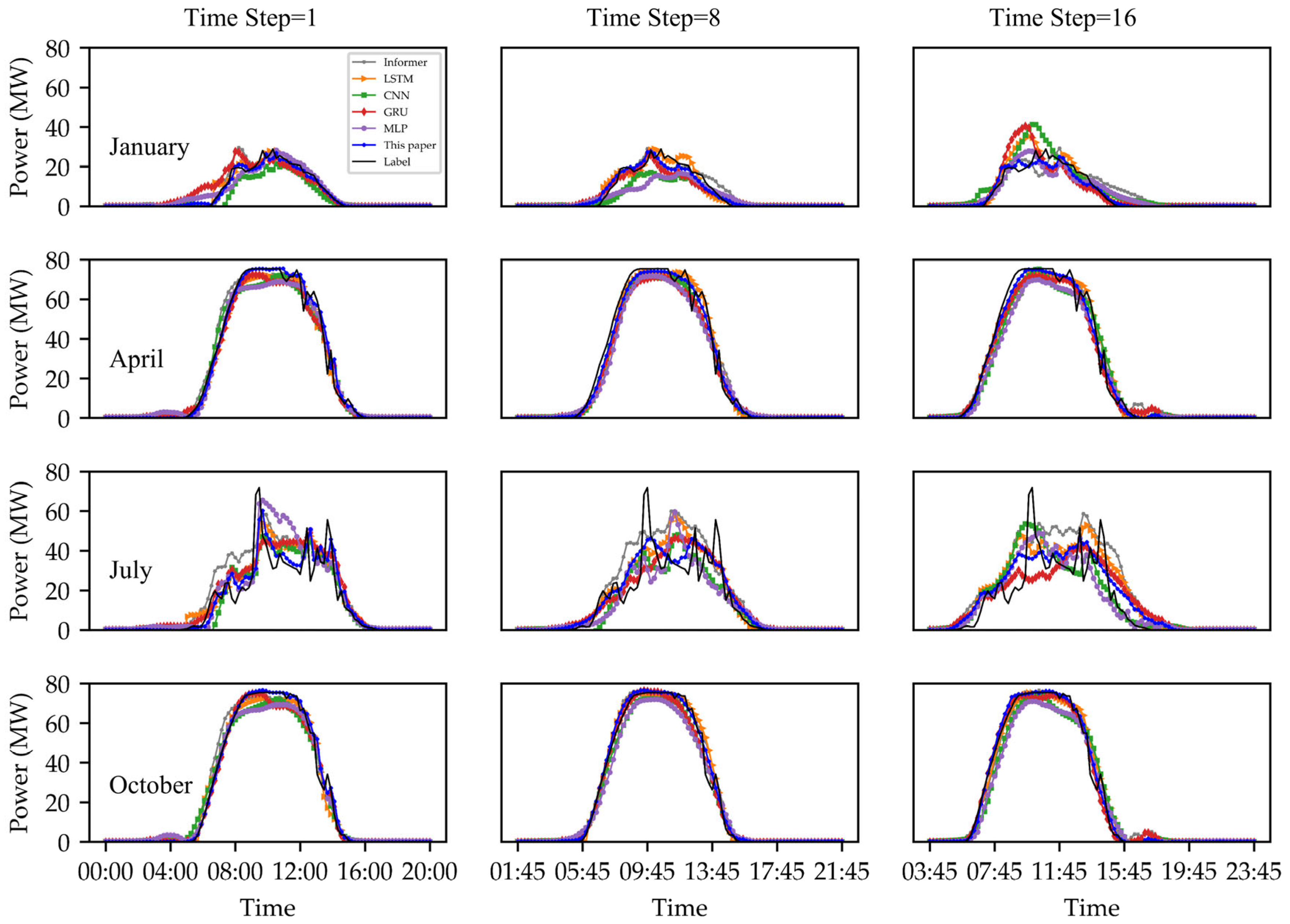
The test results of the proposed forecasting framework were compared with five benchmark models. Figure 7 shows the prediction curves of six methods on typical days across four seasons. Since the proposed framework models each time step separately, it can learn different weights for different time steps to leverage complementary strengths, resulting in more robust predictions. Regarding peak values, all benchmark models underestimated the true values. This occurs because machine learning models tend to exhibit conservative prediction behavior to minimize overall error across the training set. The proposed framework corrects benchmark predictions in the second-layer network, appropriately elevating peak forecasts to better match true values, as seen in the April and October peak intervals in the figure. For oscillation patterns, time-series deep learning models showed aggressive overestimation, while the MLP model demonstrated insufficient fitting capability. The proposed framework more closely follows the actual curve.

Table 4. Power prediction accuracy of six methods from September 2023 to February 2024 (Unit: %).

Month	9	10	11	12	1	2
Informer	88.5	93.1	91.4	91.1	89.7	90.5
LSTM	90.2	94.3	93.1	92.7	92.3	92.8
CNN	90.5	93.5	92.4	92.0	91.1	91.7
GRU	90.8	94.7	93.8	92.8	93.2	93.3
MLP	88.8	90.5	84.6	84.3	83.5	83.1
This paper	90.5	94.9	93.8	93.0	93.3	93.4

and

Table 5. Power prediction accuracy of six methods from March 2024 to August 2024 (Unit: %).

Month	3	4	5	6	7	8
Informer	90.2	90.8	90.8	87.7	88.1	86.9
LSTM	91.0	92.0	92.1	89.2	90.2	88.3
CNN	90.2	91.6	91.9	89.3	90.6	88.2
GRU	91.2	92.2	92.4	89.2	90.5	88.3
MLP	79.6	83.3	85.2	85.1	88.5	86.1
This paper	91.4	92.4	92.6	89.3	90.2	88.5

collectively present the computational performance results of six methods over a 12-month period. Results show the proposed framework achieved superior performance in 10 months. These results demonstrate that the parallel multi-model fusion framework can synthesize predictions from various models and leverage their collective experience to deliver more accurate forecasts.

Regarding different prediction time steps, the proposed framework consistently outperformed others, as shown in

Table 6. RMSE and R values of six methods across different prediction time steps.

Method	Time Step
	1		8		16
	RMSE (MW)	R	RMSE (MW)	R	RMSE (MW)	R
Informer	7.63	0.97	10.17	0.93	11.43	0.92
LSTM	7.03	0.97	9.05	0.95	10.02	0.93
CNN	7.48	0.96	9.41	0.94	10.53	0.93
GRU	6.72	0.97	9.30	0.94	10.06	0.93
MLP	8.93	0.94	10.08	0.93	16.01	0.85
This paper	5.74	0.98	8.96	0.95	9.86	0.94

. The RMSE was 5.74 MW for the first time step, 8.96 MW for the 8th step, and 9.86 MW for the 16th step. Mainstream time-series models exhibited declining accuracy with longer prediction horizons, particularly showing the lowest accuracy at the 4 h prediction mark. The proposed framework maintained a correlation of 0.98 at the first time step and 0.94 at the final step, surpassing all benchmarks. These results confirm the framework’s superior performance in both prediction accuracy and result correlation at each individual time step compared to benchmark models.

4. Conclusions

This paper proposes a multi-stage ensemble learning framework. The primary contributions lie in the strategies introduced for feature selection, model screening, and prediction result integration. For feature selection, a Recursive Feature Elimination (RFE) algorithm based on weighted scores from LightGBM, XGBoost, and MLP is employed to screen high-contribution features. In terms of model selection, mainstream power prediction models are utilized as a candidate pool. The similarity in predictive behavior among models is computed based on mutual information, and multiple categories of models with similar predictive behaviors are identified through hierarchical clustering. Guided by the principles of intra-group competition and inter-group complementarity, an optimal model combination is selected to enhance overall performance. For prediction integration, a secondary training process is applied to the predictions of the selected models, with separate modeling for different time steps to establish an adaptive weighting strategy.

In terms of feature selection, the construction of feature subsets is accomplished by recursively eliminating the least important features. For each distinct feature subset, LightGBM, XGBoost, and MLP models are trained separately, with a weighted score serving as the performance metric for that particular subset. Experiments compared three cases: employing no feature selection strategy, utilizing the feature selection strategy from the open-source library sklearn, and applying the RFE selection strategy based on LightGBM–XGBoost–MLP weighted scoring. The evaluation was conducted using data from three sites, including a 75 MW power station and the open-source PVOD dataset. The proposed method achieved optimal performance in both MAE and R² metrics. The MAE values for sites P1, P2, and P3 were 3.932 MW, 0.232 kW, and 0.951 kW, respectively, with corresponding R² values of 0.90, 0.92, and 0.90. The experimental results demonstrate that the proposed feature selection strategy has a positive impact on power forecasting.

In the aspect of model selection, to address the lack of systematic criteria and the inherent randomness and arbitrariness in traditional methods, this paper proposes a model selection strategy based on the principles of intra-group competition and inter-group complementarity. The similarity in prediction behavior among different models is quantified using mutual information, followed by hierarchical clustering to group models with similar prediction behaviors. Experiments compared three scenarios: selecting k models based on hierarchical clustering, selecting the same number of models based on Top-k accuracy, and randomly selecting k models. For sites P4, P5, and P6, the proposed model selection strategy achieved the lowest MAE values of 0.716 kW, 0.818 kW, and 1.454 kW, respectively, and the highest R² values of 0.93, 0.92, and 0.85, respectively. It is noteworthy that selecting the same number of models based on Top-k accuracy did not yield the lowest MAE or the highest R². The experimental results demonstrate that quantifying and clustering prediction behaviors to select models can enhance model diversity while preserving model disparity, thereby exerting a positive influence on final performance.

In terms of integrating model prediction outcomes, this study improves upon traditional static weighting schemes. Along the temporal dimension, separate models are constructed for each of the 16 prediction time steps to allow different models to perform optimally at appropriate time scales. For the inputs of the secondary training, initial meteorological parameters are incorporated to enable the model to learn how to make prediction decisions under varying weather conditions. Experiments compared two approaches: weighted averaging of different models and the proposed SVR-based secondary training method. For sites P7, P8, and P9, the proposed strategy achieved the lowest MAE values of 1.212 kW, 0.538 kW, and 0.774 kW, respectively, and the highest R² values of 0.87, 0.90, and 0.89, respectively. The experiments demonstrate that the proposed dynamic weighting scheme outperforms traditional static weighting strategies.

In terms of overall performance, this paper compares five mainstream power forecasting models, namely, Informer, LSTM, CNN, GRU, and MLP. Over a one-year dataset, the proposed model achieved optimal performance in 10 months. Across different prediction time steps, it exhibited superior correlation (0.94–0.98) and lower RMSE (5.74–9.86 MW) compared to baseline models. The experiments demonstrate that the proposed multi-stage ensemble learning framework—which synergistically optimizes feature selection, model screening, and dynamic weighted integration—enhances both the accuracy and robustness of power forecasting.

References

1. Barhmi, K.; Heynen, C.; Golroodbari, S.; van Sark, W. A Review of Solar Forecasting Techniques and the Role of Artificial Intelligence. Solar 2024, 4, 99–135. [Google Scholar] [CrossRef]
2. Iheanetu, K.J. Solar Photovoltaic Power Forecasting: A Review. Sustainability 2022, 14, 17005. [Google Scholar] [CrossRef]
3. Yang, D.; Wang, W.; Gueymard, C.A.; Hong, T.; Kleissl, J.; Huang, J.; Perez, M.J.; Perez, R.; Bright, J.M.; Xia, X.A.; et al. A review of solar forecasting, its dependence on atmospheric sciences and implications for grid integration: Towards carbon neutrality. Renew. Sustain. Energy Rev. 2022, 161, 112348. [Google Scholar] [CrossRef]
4. Malinkovich, Y.; Sitbon, M.; Lineykin, S.; Dagan, K.J.; Baimel, D. A Combined Persistence and Physical Approach for Ultra-Short-Term Photovoltaic Power Forecasting Using Distributed Sensors. Sensors 2024, 24, 2866. [Google Scholar] [CrossRef] [PubMed]
5. Dou, Y.; Tan, S.; Xie, D. Comparison of machine learning and statistical methods in the field of renewable energy power generation forecasting: A mini review. Front. Energy Res. 2023, 11, 1218603. [Google Scholar] [CrossRef]
6. Lateko, A.A.H.; Yang, H.-T.; Huang, C.-M. Short-Term PV Power Forecasting Using a Regression-Based Ensemble Method. Energies 2022, 15, 4171. [Google Scholar] [CrossRef]
7. Theocharides, S.; Theristis, M.; Makrides, G.; Kynigos, M.; Spanias, C.; Georghiou, G.E. Comparative Analysis of Machine Learning Models for Day-Ahead Photovoltaic Power Production Forecasting. Energies 2021, 14, 1081. [Google Scholar] [CrossRef]
8. Marion, W.; George, R. Calculation of solar radiation using a methodology with worldwide potential. Sol. Energy 2001, 71, 275–283. [Google Scholar] [CrossRef]
9. Ineichen, P. A broadband simplified version of the Solis clear sky model. Sol. Energy 2008, 82, 758–762. [Google Scholar] [CrossRef]
10. Yang, D. Choice of clear-sky model in solar forecasting. J. Renew. Sustain. Energy 2020, 12, 026101. [Google Scholar] [CrossRef]
11. Kim, D.; Ramanathan, V. Solar radiation budget and radiative forcing due to aerosols and clouds. J. Geophys. Res. Atmos. 2008, 113. [Google Scholar] [CrossRef]
12. Boyd, M.T.; Klein, S.A.; Reindl, D.T.; Dougherty, B.P. Evaluation and Validation of Equivalent Circuit Photovoltaic Solar Cell Performance Models. J. Sol. Energy Eng. 2011, 133, 021005. [Google Scholar] [CrossRef]
13. Raya-Armenta, J.M.; Ortega, P.R.; Bazmohammadi, N.; Spataru, S.V.; Vasquez, J.C.; Guerrero, J.M. An Accurate Physical Model for PV Modules with Improved Approximations of Series-Shunt Resistances. IEEE J. Photovolt. 2021, 11, 699–707. [Google Scholar] [CrossRef]
14. Zhi, Y.; Sun, T.; Yang, X. A physical model with meteorological forecasting for hourly rooftop photovoltaic power prediction. J. Build. Eng. 2023, 75, 106997. [Google Scholar] [CrossRef]
15. Shadab, A.; Ahmad, S.; Said, S. Spatial forecasting of solar radiation using ARIMA model. Remote Sens. Appl. Soc. Environ. 2020, 20, 100427. [Google Scholar] [CrossRef]
16. Du, X.; Lang, Z.; Liu, M.; Wu, J. Regression analysis and prediction of monthly wind and solar power generation in China. Energy Rep. 2024, 12, 1385–1402. [Google Scholar] [CrossRef]
17. Kim, Y.S.; Joo, H.Y.; Kim, J.W.; Jeong, S.Y.; Moon, J.H. Use of a Big Data Analysis in Regression of Solar Power Generation on Meteorological Variables for a Korean Solar Power Plant. Appl. Sci. 2021, 11, 1776. [Google Scholar] [CrossRef]
18. Suksamosorn, S.; Hoonchareon, N.; Songsiri, J. Post-Processing of NWP Forecasts Using Kalman Filtering With Operational Constraints for Day-Ahead Solar Power Forecasting in Thailand. IEEE Access 2021, 9, 105409–105423. [Google Scholar] [CrossRef]
19. Chodakowska, E.; Nazarko, J.; Nazarko, Ł.; Rabayah, H.S.; Abendeh, R.M.; Alawneh, R. ARIMA Models in Solar Radiation Forecasting in Different Geographic Locations. Energies 2023, 16, 5029. [Google Scholar] [CrossRef]
20. Olcay, K.; Gíray Tunca, S.; Aríf Özgür, M. Forecasting and Performance Analysis of Energy Production in Solar Power Plants Using Long Short-Term Memory (LSTM) and Random Forest Models. IEEE Access 2024, 12, 103299–103312. [Google Scholar] [CrossRef]
21. Li, X.; Ma, L.; Chen, P.; Xu, H.; Xing, Q.; Yan, J.; Lu, S.; Fan, H.; Yang, L.; Cheng, Y. Probabilistic solar irradiance forecasting based on XGBoost. Energy Rep. 2022, 8, 1087–1095. [Google Scholar] [CrossRef]
22. Das, U.K.; Tey, K.S.; Idris, M.Y.I.B.; Mekhilef, S.; Seyedmahmoudian, M.; Stojcevski, A.; Horan, B. Optimized Support Vector Regression-Based Model for Solar Power Generation Forecasting on the Basis of Online Weather Reports. IEEE Access 2022, 10, 15594–15604. [Google Scholar] [CrossRef]
23. Sabzehgar, R.; Amirhosseini, D.Z.; Rasouli, M. Solar power forecast for a residential smart microgrid based on numerical weather predictions using artificial intelligence methods. J. Build. Eng. 2020, 32, 101629. [Google Scholar] [CrossRef]
24. Akhter, M.N.; Mekhilef, S.; Mokhlis, H.; Almohaimeed, Z.M.; Muhammad, M.A.; Khairuddin, A.S.M.; Akram, R.; Hussain, M.M. An Hour-Ahead PV Power Forecasting Method Based on an RNN-LSTM Model for Three Different PV Plants. Energies 2022, 15, 2243. [Google Scholar] [CrossRef]
25. Ait Mansour, A.; Tilioua, A.; Touzani, M. Bi-LSTM, GRU and 1D-CNN models for short-term photovoltaic panel efficiency forecasting case amorphous silicon grid-connected PV system. Results Eng. 2024, 21, 101886. [Google Scholar] [CrossRef]
26. Jung, Y.; Jung, J.; Kim, B.; Han, S. Long short-term memory recurrent neural network for modeling temporal patterns in long-term power forecasting for solar PV facilities: Case study of South Korea. J. Clean. Prod. 2020, 250, 119476. [Google Scholar] [CrossRef]
27. Limouni, T.; Yaagoubi, R.; Bouziane, K.; Guissi, K.; Baali, E.H. Accurate one step and multistep forecasting of very short-term PV power using LSTM-TCN model. Renew. Energy 2023, 205, 1010–1024. [Google Scholar] [CrossRef]
28. Tao, K.; Zhao, J.; Tao, Y.; Qi, Q.; Tian, Y. Operational day-ahead photovoltaic power forecasting based on transformer variant. Appl. Energy 2024, 373, 123825. [Google Scholar] [CrossRef]
29. Kim, J.; Obregon, J.; Park, H.; Jung, J.-Y. Multi-step photovoltaic power forecasting using transformer and recurrent neural networks. Renew. Sustain. Energy Rev. 2024, 200, 114479. [Google Scholar] [CrossRef]
30. Sharma, N.; Mangla, M.; Yadav, S.; Goyal, N.; Singh, A.; Verma, S.; Saber, T. A sequential ensemble model for photovoltaic power forecasting. Comput. Electr. Eng. 2021, 96, 107484. [Google Scholar] [CrossRef]
31. AlKandari, M.; Ahmad, I. Solar power generation forecasting using ensemble approach based on deep learning and statistical methods. Appl. Comput. Inform. 2020, 20, 231–250. [Google Scholar] [CrossRef]
32. Nastić, F.; Jurišević, N.; Nikolić, D.; Končalović, D. Harnessing open data for hourly power generation forecasting in newly commissioned photovoltaic power plants. Energy Sustain. Dev. 2024, 81, 101512. [Google Scholar] [CrossRef]
33. Yao, T.; Wang, J.; Wu, H.; Zhang, P.; Li, S.; Wang, Y.; Chi, X.; Shi, M. PVOD v1.0: A Photovoltaic Power Output Dataset; Science Data Bank: Beijing, China, 2021. [Google Scholar]
Figure 1. Photovoltaic power prediction framework based on multi-stage ensemble learning.
Energies 18 04644 g001
Figure 2. Flowchart of the RFE feature selection method with LightGBM–XGBoost–MLP weighting.
Energies 18 04644 g002
Figure 3. Adaptive model selection framework based on hierarchical clustering.
Energies 18 04644 g003
Figure 4. Flowchart of 5-fold cross-validation training.
Energies 18 04644 g004
Figure 5. Secondary feature construction based on primary prediction results and meteorological data.
Energies 18 04644 g005
Figure 6. Schematic diagram of secondary fusion learning across different time steps.
Energies 18 04644 g006
Figure 7. Prediction curves of six methods on typical days across four seasons.
Energies 18 04644 g007