Research on Transmission Line Icing Prediction for Power System Based on Improved Snake Optimization Algorithm-Optimized Deep Hybrid Kernel Extreme Learning Machine

Abstract

As extreme weather events become more frequent, the icing of transmission lines in winter has become more common, causing significant economic losses to power systems and drawing increasing attention. However, owing to the complexity of the conductor icing process, establishing high-precision ice thickness prediction models is vital for ensuring the safe and stable operation of power grids. Therefore, this paper proposes a hybrid model combining an improved snake optimization (ISO) algorithm, deep extreme learning machine (DELM), and hybrid kernel extreme learning machine (HKELM). Firstly, based on the analysis of the factors that influence the icing, the temperature, the humidity, the wind velocity, the wind direction, and the precipitation are selected as the weather parameters for the prediction model of the transmission line icing. Secondly, the HKELM is introduced into the regression layer of DELM to obtain the deep hybrid kernel extreme learning machine (DHKELM) model for ice thickness prediction. The SO algorithm is then augmented by incorporating the Latin hypercube sampling technique, t-distribution mutation strategy, and Cauchy mutation, enhancing its convergence. Finally, the ISO-DHKELM model is applied to the icing data of transmission lines in Sichuan Province for experiments. The simulation results indicate that this model not only performs well, but also enhances the accuracy of ice thickness predictions.

1. Introduction

With the increasing severity of global warming, the occurrence rate of extreme weather events has been growing, inflicting substantial damage on the national economy. Among these adverse meteorological phenomena, icing of transmission lines is one of the most severe disasters in power systems, posing a significant threat to the safety and stability of electricity networks. The history of transmission line icing accidents dates back to 1932, and since then, such disasters have successively struck countries and regions including Russia, Canada, the United States, the United Kingdom, and China [1,2,3,4]. Given that power systems are complex lifeline projects with the transmission link being of utmost importance, any problem in this link can severely disrupt the order of production and life, leading to incalculable losses. Along with the continuous increase in the demand for power, the harm caused by the combination of ice and other loads on the large span high voltage transmission line is becoming more and more serious. Therefore, conducting research on transmission line icing is of great significance.

In recent years, domestic and international researchers have extensively studied transmission-line icing, and research content and methods have advanced in step with technological progress. Current icing-prediction methods fall into three main categories: physical models, statistical approaches, and machine-learning models. Physical models, such as the Imai, Lenhard, and Makkonen models [5,6], exhibit notable differences. The Imai model focuses on heat and mass transfer and on the energy balance at the ice–air interface; it is suitable for preliminary predictions under stable weather but tends to underestimate ice thickness in high winds. The Lenhard model emphasizes the dynamics of droplet impact and employs empirical adhesion coefficients; it accurately describes the accumulation of large droplets but requires site-specific parameter calibration. The Makkonen model integrates thermodynamic and dynamic processes into a multi-factor framework that offers broader applicability, though its complex parameters complicate implementation. All three models differ in how they calculate ice-growth rate, process heat exchange, and apply correction coefficients.

Nevertheless, accurately predicting ice thickness remains challenging because key parameters such as droplet radius and adhesion coefficients are difficult to measure during icing events, which limits practical application. To address these limitations, conventional statistical methods, including multiple linear regression, time-series analysis, and extreme-value theory [7,8,9], have been adopted. However, these approaches rely on numerous statistical assumptions, struggle to incorporate micro-meteorological factors, and consequently suffer from low accuracy and limited applicability.

Compared with traditional physical and statistical methods, machine learning has significantly enhanced prediction accuracy by deeply exploring the complex nonlinear relationships between ice thickness and meteorological factors such as temperature, humidity, and wind speed, thus becoming a powerful tool in the field of ice thickness prediction [10,11]. In the early stages of exploration, artificial neural network technologies, such as back propagation (BP) neural networks and support vector machines (SVMs), quickly became research hotspots due to their strong data processing capabilities [12,13]. For instance, Reference [14] presented a framework utilizing the adaptive relevance vector machine (ARVM) to predict icing fault probabilities, achieving enhanced predictive accuracy. The application of a back propagation (BP) neural network architecture for the purpose of short-term icing forecasting was explored in the work by [15]. Nevertheless, these methodologies exhibit certain limitations; notably, the BP network is susceptible to premature convergence to local optima, while support vector machines (SVMs) can be computationally intensive. To address these issues, scholars have introduced optimization algorithms for improvement. Reference [16] proposed an innovative prediction model based on the generalized regression neural network (GRNN) and the fruit fly optimization algorithm (FOA) to enhance the accuracy and stability of icing prediction. Reference [17] presented a galloping prediction model for iced transmission lines based on the Particle swarm optimization-conditional generative adversarial network (PSO-CGAN). The research in [18] led to the formulation of the weighted support vector machine regression (WSVR), a specifically modified and improved framework based on conventional SVM regression principles. Through the application of a hybridized swarm intelligence approach, which integrates particle swarm optimization (PSO) with ant colony optimization (ACO) for parameter tuning, a notable improvement in the model’s predictive performance was achieved. An ice accretion forecasting system was put forth in [19], constructed upon a hybridization of the fireworks algorithm and the weighted least squares support vector machine (W-LSSVM). This integration was designed to harness the complementary advantages of both methodologies, resulting in enhanced predictive outcomes. A hybrid modeling approach was examined in [20], wherein a wavelet support vector machine (w-SVM) was coupled with the quantum fireworks algorithm (QFA) to achieve superior predictive capabilities. Reference [21] proposed A BOA-VMD-LSTM hybrid model, which demonstrated superior performance.

Compared with the aforementioned methods, the extreme learning machine (ELM) method can overcome their shortcomings. It effectively reduces the risk of falling into local optima while significantly enhancing the learning speed and generalization ability. Therefore, ELM has been widely applied in the field of prediction and has achieved satisfactory results in most cases [22,23]. However, the random initialization of weights and biases limits its performance. To address this issue, scholars have adopted various improvement methods. The work in Reference [24] utilized the kernel extreme learning machine (KELM) to address the issue of model instability and to improve its predictive precision.

Table 1. Comparison of machine learning methods.

Algorithms	Core Features	Strengths	Weaknesses
BP	Multi-layer feed-forward network with back-propagation weight updates.	Simple to implement; can approximate any non-linear mapping.	Prone to local minima; slow training; suffers from vanishing gradients.
SVM	Max-margin kernel classifier mapping data to high-D space.	Global optimum, robust to high-dim small samples.	High cost for large data; kernel tuning needed.
ARVM	Adaptive sparse Bayesian kernel model with automatic kernel-parameter tuning.	More sparsity, probabilistic output, robust for high-dim small samples.	Slow training, complex hyper-parameters.
GRNN	One-pass radial-basis memory network that stores all training samples.	Extremely fast training, smooth approximation, good for small datasets.	Must store all samples with high memory usage, poor scalability to big data.
ELM	Single-hidden-layer feed-forward network; hidden weights are randomly fixed and only the output layer is trained.	Extremely fast training; almost no parameter tuning.	Random weights cause unstable results; requires a large number of hidden neurons.
HKELM	ELM with hybrid kernel trained in one step, eliminating the need to set hidden-layer nodes.	Fast training, high accuracy, captures both global and local patterns.	Hybrid-kernel parameters must be tuned; memory and computation explode with large datasets.

will provide a detailed comparative description of the above-mentioned machine-learning algorithms.

Intelligent optimization algorithms have provided new ideas for the parameter optimization of machine learning models. Among these algorithms, the snake optimization (SO) algorithm stands out. It models the feeding, mating, and combat behaviors of male and female snakes in different scenarios of food supply and temperature [25]. Based on the living habits of snakes, the algorithm is divided into exploration and exploitation phases. Many scholars, both domestically and internationally, have investigated this algorithm and found that compared to other algorithms, it effectively balances local and global aspects of the problem. During the search process, these two aspects can transform into each other, thus avoiding local optima and achieving better convergence. Thanks to its excellent global search capability, SO has been successfully applied in various fields [26,27]. Additionally, from the perspective of combining a deep hidden layer kernel extreme learning machine (DHKELM) with optimization algorithms [28], few researchers have applied it to conductor icing forecast. Therefore, this paper employs a hybrid model to predict transmission line icing.

The primary contributions of this study can be summarized as follows:

• This study puts forth an improved snake optimization algorithm (ISO). The optimization capabilities of this algorithm are augmented through the integration of three distinct mechanisms: Latin hypercube sampling, a t-distribution mutation operator, and a Cauchy mutation strategy.
• A DHKELM is constructed, combining the deep feature extraction of DELM and the kernel mapping advantages of HKELM to improve the model’s expressive ability.
• The ISO-DHKELM hybrid prediction model was constructed and demonstrated superior performance in ice prediction, achieving RMSE, MAE, and R² values of 0.057, 0.044, and 0.993, respectively. This provides a novel approach for power grid ice disaster prevention and mitigation.

The structure of this paper is organized as follows: Section 2 systematically elaborates the theoretical foundations of the relevant models and algorithms; Section 3 delves into the analysis of data characteristics and processing methods; Section 4 validates the effectiveness of the model through experiments; and Section 5 summarizes the main conclusions of the research and provides an outlook for future research directions.

2. Methodology

2.1. HKELM

ELM is a feed-forward neural network with a single hidden layer [29]. Compared with the conventional neural network, the hidden layer bias is initialized at random, and the output layer consists only of weights. ELM is different from the traditional training method based on gradient. It uses a linear system to solve the weights of the output layer. The typical network configuration is shown in Figure 1.

Expressed by Equation (1):

$$\begin{array}{c}f\left(x\right)=H\beta \end{array}$$

(1)

In this context, b denotes the output weight vector. Its value is determined via the formulation presented in Equation (2), which involves the computation of H⁺, defined as the Moore–Penrose pseudoinverse of the hidden layer’s output matrix.

$$\begin{array}{c}\left\{\begin{array}{c}\beta =H^{+}T\\ H^{+}=H^T{\left({HH}^T+{\displaystyle \frac{I}{C}}\right)}^{-1}\end{array}\right.\end{array}$$

(2)

where $H^{+}$ is the Moore–Penrose generalized inverse matrix, T is the real value, the positive constant C is the penalty parameter, and I is the unit matrix.

Detailed ELM description:

$$\begin{array}{c}f\left(x\right)=H{H}^T{\left({\displaystyle \frac{I}{C}}+H{H}^T\right)}^{-1}T\end{array}$$

(3)

To enhance the learning capacity, generalization performance, and operational stability of the conventional ELM, a kernel function, K(·), is integrated into the framework, thereby formulating the kernel extreme learning machine (KELM) model, as mathematically defined in Equation (4).

$$\begin{array}{c}{f}_{KELM}=H{H}^T; f_{KELM}=h\left(x_i\right)h\left(x_j\right)=K\left(x_i,x_j\right)\end{array}$$

(4)

The KELM may be further expressed as follows:

$$\begin{array}{c}f\left(x\right)={\left[\begin{array}{c}K\left(x,x_i\right)\\ ⋮\\ K\left(x,x_N\right)\end{array}\right]\left({\displaystyle \frac{I}{C}}+f_{KELM}\right)}^{-1}T\end{array}$$

(5)

The transformational capacity of a kernel extreme learning machine (KELM) is fundamentally dictated by its kernel function. These functions fall into a dichotomy of local and global types, each presenting a distinct trade-off. Kernels with a local scope are highly adept at modeling granular, localized data patterns, but this specialization often comes at the cost of limited generalization performance on unseen data. Conversely, global kernels are effective at capturing overarching data trends but may exhibit a reduced capacity to learn intricate, complex relationships within the data. The Gaussian kernel $K_{RBF}\left(x,x_i\right)$ and a polynomial kernel function $K_{poly}(x,x_i)$ are widely used local and global kernel functions, respectively, with expressions as follows:

$$\begin{array}{c}\left\{\begin{array}{c}{K}_{RBF}\left(x,x_i\right)=\exp \left(-{\displaystyle \frac{{‖x,x_i‖}^2}{2{\sigma }^2}}\right)\\ K_{poly}\left(x,x_i\right)={\left(\left(x.x_i\right)+q\right)}^p\end{array}\right.\end{array}$$

(6)

where γ = $2{\sigma }^2$ represents the kernel parameter where q denotes a constant tuning parameter, and p represents the degree of the polynomial kernel. A composite kernel is formulated by linearly combining the Gaussian and polynomial kernel functions. This approach fully utilizes the benefits of each core function, yielding better fault diagnosis results than using a single kernel function [30]. The composite kernel is thus defined as follows:

$$\begin{array}{c}K\left(x,x_i\right)=v.K_{RBF}+\left(1-v\right).K_{poly}, v\in [0, 1]\end{array}$$

(7)

where in v represents the weighting coefficient that balances the contribution of each base kernel within the composite function.

2.2. ELM-AE

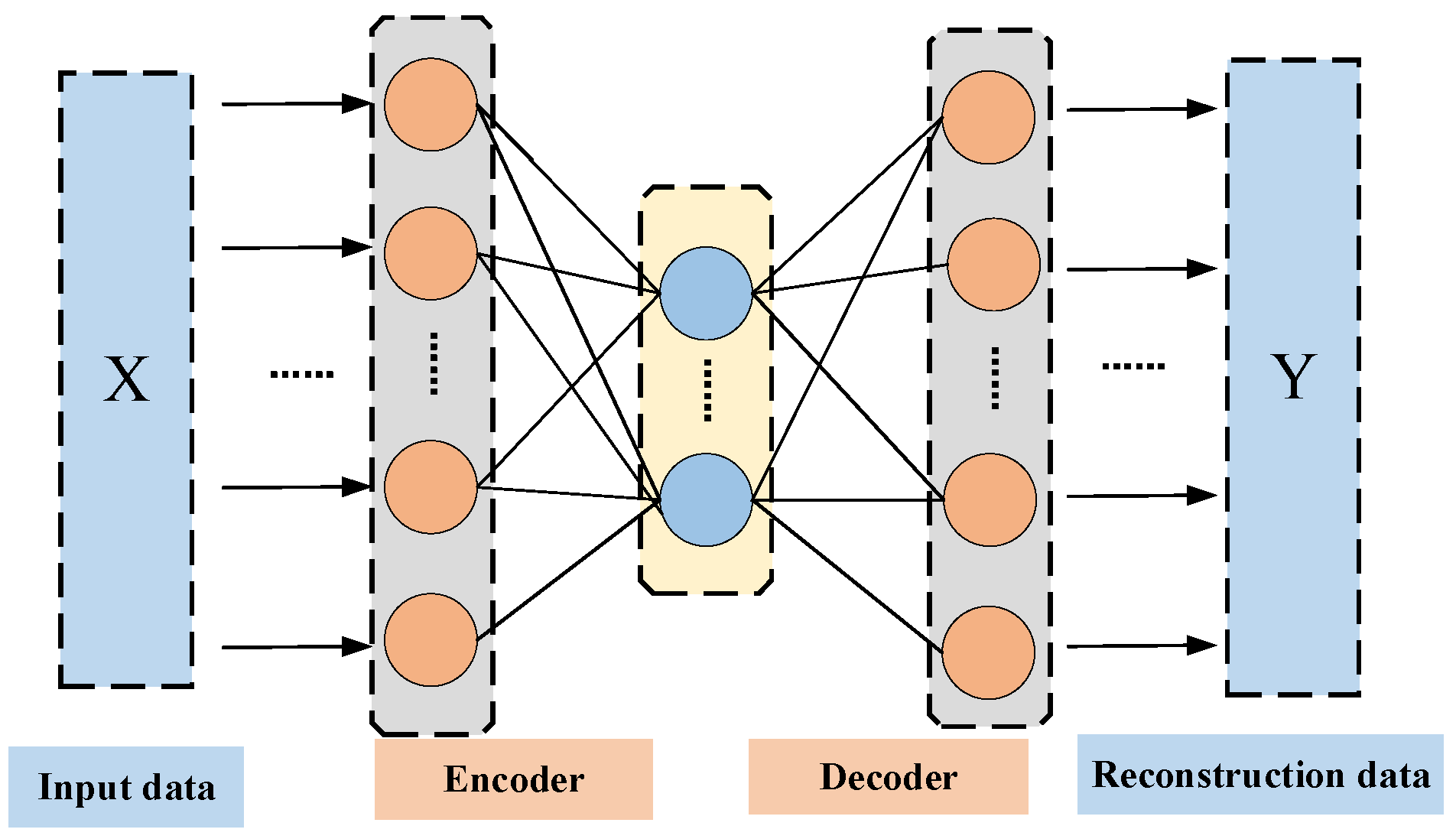
Autoencoder (AE) denotes an unsupervised neural network used in deep learning to establish mappings via input data supervision, as shown in Figure 2. However, it suffers from slow training and susceptibility to local optima. Researchers combined AE with ELM to create ELM-AE, which retains ELM’s characteristics of random initialization and orthogonalization of weights and biases. Based on the Johnson–Lindenstrauss theorem, this approach transforms input data into different dimensional spaces to create feature representations. Compared to AE, ELM-AE has stronger mapping and generalization abilities [31].

2.3. DHKELM

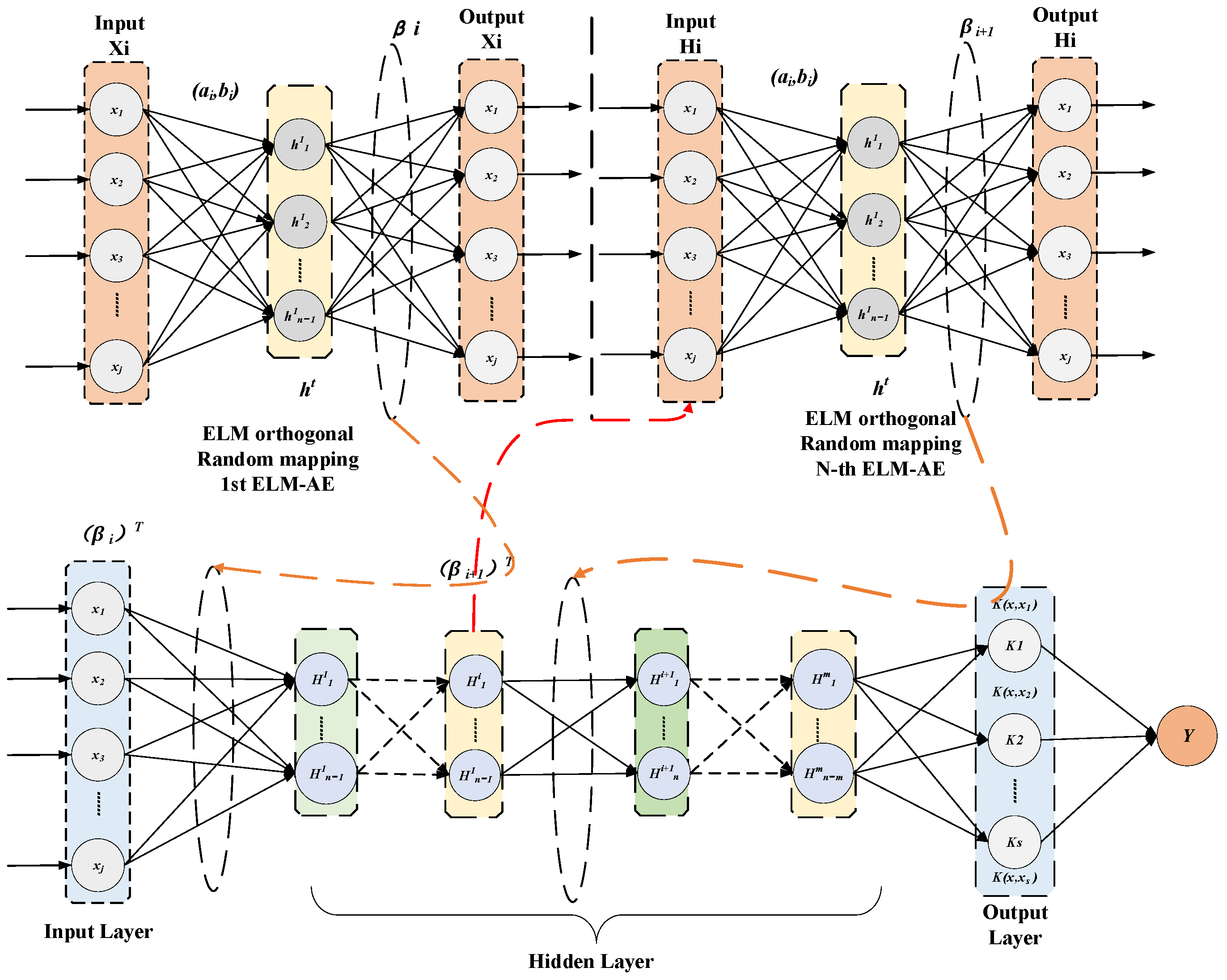
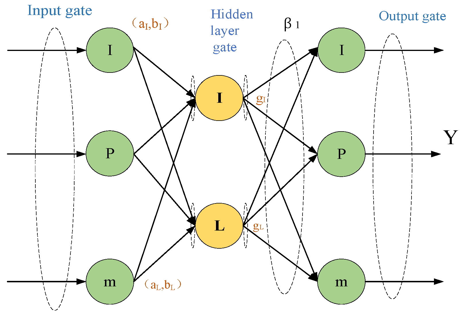
The model is based on ELM-AE and ELM is used as the final regression layer. The DHKELM model is obtained by replacing DELM’s original regression layer with HKELM [32]. The algorithm has two stages: unsupervised and supervised. In the unsupervised stage, ELM-AE learns high-level data features, extracting simple to complex features and saving the output weight matrix. In the supervised stage, HKELM serves as the regression layer, combining label information to optimize weights and improve prediction accuracy. The DHKELM network structure, shown in Figure 3. The hidden layer state matrix is represented by Equation (8):

$$\begin{array}{c}{h}^t={\left[{\left({\displaystyle \frac{I}{C}}+H{H}^T\right)}^{-1}\right]}^T\end{array}$$

(8)

The weight is given by Equation (9) as below.

$$\begin{array}{c}{\beta }^{i+1}={\left({\displaystyle \frac{I}{C}}+{\left(h_t\right)}^T{h}_t\right)}^{-1}{\left(h_t\right)}^T\end{array}$$

(9)

Features are propagated between layers through an extraction mechanism. The output $H^i$ of the prior layer acts as the input $H^{i+1}$ for the subsequent layer, as specified in Equation (10).

$$\begin{array}{c}{H}^0=X\end{array}$$

(10)

$$\begin{array}{c}{H}^{i+1}=g({({\beta }^{i+1})}^T{H}^i)\end{array}$$

(11)

Architecturally, the hierarchical kernel extreme learning machine (HKELM) performs predictive regression using features synthesized from its M antecedent hidden layers. In contrast, for the deep extreme learning machine (DELM), the output weight matrix is determined via a least squares estimation aimed at minimizing a regularized objective function, a process mathematically formulated in Equation (12).

$$\begin{array}{c}Y=g\left(a^{in}{H}^m+b^{in}\right)\end{array}$$

(12)

2.4. Snake Optimization Algorithm

Motivated by the distinctive courtship rituals of serpents, Hashim et al. [26] proposed the SO algorithm. This algorithm recreates the behaviors of food procurement, reproduction, and aggression by snakes, which are contingent upon the variations in food accessibility and temperature. Based on the living habits of snakes, it is divided into exploration and exploitation phases.

2.4.1. Population Initialization Phase

Similar to all metaheuristic approaches, the SO initiates by generating a randomly distributed population to commence the optimization task. The initial population is calculated based on the following formula:

$$\begin{array}{c}{X}_i=X_{min}+r\left(X_{max}-X_{min}\right)\end{array}$$

(13)

where $X_i$ represents the position, r is an incidental value from 0 to 1, and $X_{min}$, $X_{max}$ represent lower and upper bounds of the population, respectively.

2.4.2. Split the Snake into Equal Groups of Females and Males

Suppose half of the population consists of males and the other half of females, the population is divided into two separate groups: the male assembly and the female assembly, as delineated by the subsequent formula:

$$\begin{array}{c}{N}_m\approx {\displaystyle \frac{N}{2}}\end{array}$$

(14)

$$\begin{array}{c}{N}_f=N-N_m\end{array}$$

(15)

where N is indicative of the entire population size in terms of individuals, $N_m$ signifies the count of males within the population, and $N_f$ signifies the count of females within the population.

2.4.3. Assess Each Cluster and Identify the Temperature

Following a group-based fitness evaluation, a selection process identifies the elite male (X_best_m) and female (X_best_f) solutions, along with the current optimal resource location (X_food). Concurrently, a dynamic control parameter, temperature (T), is updated according to the subsequent mathematical expression:

$$\begin{array}{c}Temp=\mathit{exp}({\displaystyle \frac{-t}{T}})\end{array}$$

(16)

where t represents the current iteration, and T represents the maximum number of iterations.

The quantity of food (Q), which can be obtained through the following equation:

$$\begin{array}{c}Q=c_1\times \mathit{exp}({\displaystyle \frac{t-T}{T}})\end{array}$$

(17)

where $c_1$= 0.5.

2.4.4. Exploration Phase (Without Food)

If Q < Threshold (Threshold = 0.25), snakes will haphazardly choose a place to hunt for sustenance and modify their positions as needed. For the model’s exploration phase, as governed by the subsequent expression:

$$\begin{array}{c}{X}_{i,m}(t+1)=X_{rand,m}\left(t\right)\pm c_2\times A_m\times \left(\right(X_{max}-X_{min})\times \mathrm{rand}+X_{min})\end{array}$$

(18)

where $X_{i,m}$ denotes the location, $X_{rand,m}$ indicates the location of an arbitrarily chosen male, with rand being a stochastic value from 0 to 1, and $c_2$ = 0.05.

The orientation indicator function, referred to as the variability factor, allows for the potential to augment or diminish the position outcome, thus conducting a good search in all possible directions of the given search space. This parameter is randomly generated to achieve randomness. $A_m$ represents the capacity of males to look for food, as illustrated by the subsequent equation:

$$\begin{array}{c}{A}_m=\mathit{exp}({\displaystyle \frac{-f_{rand,m}}{f_{i,m}}})\end{array}$$

(19)

where $f_{rand,m}$ denotes the fitness of $X_{rand,m}$, and $f_{i,m}$ represents the fitness in the male group.

$$\begin{array}{c}{X}_{i,f}(t+1)=X_{\mathrm{rand},f}\left(t\right)\pm c_2\times A_f\times \left(\right(X_{max}-X_{min})\times \mathrm{rand}+X_{min})\end{array}$$

(20)

where $X_{i,f}$ shows the position of the i-th female, $X_{rand,f}$ reflects the position of a randomly selected female, and $A_f$ represents the capacity of females to look for food, as illustrated by the ensuing equation:

$$\begin{array}{c}{A}_f=\mathit{exp}({\displaystyle \frac{-f_{rand,f}}{f_{i,f}}})\end{array}$$

(21)

where $f_{rand,f}$ is the fitness of $X_{rand,f}$, and $f_{i,f}$ is the fitness in the female group.

2.4.5. Exploitation Phase (Food Present)

If Q > Threshold:

If the temperature > Threshold (0.6):

Snakes advance towards the food:

$$\begin{array}{c}{X}_{i,j}\left(t+1\right)=X_{food}\pm c_3\times Temp\times rand\times \left(X_{food}-X_{i,j}\left(t\right)\right)\end{array}$$

(22)

where $X_{i,j}$ denotes the position of a male or female individual, $X_{food}$ represents the position.

If the temperature < Threshold (0.6):

Snakes will be in either a combat pattern or a breeding pattern.

Combat pattern:

$$\begin{array}{c}{X}_{i,m}\left(t+1\right)=X_{i,m}\left(t\right)+c_3\times FM\times rand\times \left(Q\times X_{best,f}-X_{i,m}\left(t\right)\right)\end{array}$$

(23)

where $X_{i,m}$ is the position of the i-th male individual, $X_{best,f}$ refers to the position, and $FM$ refers to the combat ability of the male individual.

$$\begin{array}{c}FM=\mathit{exp}({\displaystyle \frac{-f_{best,f}}{f_i}})\end{array}$$

(24)

where $f_{best,f}$ refers to the fitness value, and $f_i$ is the target fitness.

$$\begin{array}{c}{X}_{i,f}\left(t+1\right)=X_{i,f}\left(t\right)+c_3\times MM\times rand\times \left(Q\times X_{best,m}-{X_{i,}}_f\left(t\right)\right)\end{array}$$

(25)

where $X_{i,f}$ is the position of the i-th female individual, $X_{best,m}$ refers to the position in the male group, and $MM$ refers to the combat ability of the female individual.

$$\begin{array}{c}MM=\mathit{exp}({\displaystyle \frac{-f_{best,m}}{f_i}})\end{array}$$

(26)

where $f_{best,m}$ indicates the fitness, and $f_i$ represents the objective fitness value.

Breeding pattern:

$$\begin{array}{c}{X}_{i,m}\left(t+1\right)=X_{i,m}\left(t\right)+c_3\times M_m\times rand\times \left(Q\times X_{i,f}\left(t\right)-X_{i,m}\left(t\right)\right)\end{array}$$

(27)

$$\begin{array}{c}{X}_{i,f}\left(t+1\right)={X_{i,}}_f\left(t\right)+c_3\times M_f\times rand\times \left(Q\times X_{i,m}\left(t\right)-X_{i,f}\left(t\right)\right)\end{array}$$

(28)

where $M_m$ and $M_f$ denote the reproductive capabilities of males and females, respectively, and can be determined by the subsequent equation:

$$\begin{array}{c}{M}_m=\mathit{exp}({\displaystyle \frac{-f_{i,f}}{f_{i,m}}})\end{array}$$

(29)

$$\begin{array}{c}{M}_f=\mathit{exp}({\displaystyle \frac{-f_{i,m}}{f_{i,f}}})\end{array}$$

(30)

Should the eggs hatch, pick out the least desirable male and female and substitute them.

$$\begin{array}{c}{X}_{worst,m}=X_{min}+rand\times (X_{max}-X_{min})\end{array}$$

(31)

$$\begin{array}{c}{X}_{worst,f}=X_{min}+rand\times (X_{max}-X_{min})\end{array}$$

(32)

where $X_{worst,m}$ and $X_{worst,f}$ represent the worst individuals.

The pseudo-code of the SO algorithm in this paper is presented in Algorithm 1.

Algorithm 1: Snake Optimization (SO) Algorithm

1. for i = 1 to N do

2.      for j = 1 to D do

3.          X_i,j ← lb_j + rand (0, 1) × (ub_j − lb_j)

4.      end for

5.      f_i ← Calculate Fitness(X_i)

6. end for

7. [f_best, idx] ← min(f_i)

8. X_best ← X_idx

9. t ← 1

10. while t ≤ T do

11.      for i = 1 to N do

12.            if rand (0,1) < p then

13.                X_i ← X_best + α × randn() × (X_i − X_best)

14.            else

15.              X_i ← X_i + β × randn() × (ub − lb)

16.            end if

17.              X_i ← max(lb, min(X_i, ub))

18.              f_new ← CalculateFitness(X_i)

19.              if f_new < f_i then

20.                  X_i ← X_new /

21.                  f_i ← f_new

22.            end if

23.            end for

24.      [f_current_best, idx] ← min(f_i)

25.      if f_current_best < f_best then

26.        f_best ← f_current_best

27.        X_best ← X_idx

28.      end if

29.      t ← t + 1

30. end while

31. return X_best, f_best

2.5. Improved Snake Algorithm

SO is a highly optimized algorithm, yet it tends to fall into local optima, indicating a lack of global optimization capability. Consequently, to establish a more effective equilibrium between global search capabilities and local refinement, improve the convergence rate, and augment the algorithm’s overall robustness, several modifications are introduced.

2.5.1. Latin Hypercube Sampling

Latin hypercube sampling (LHS) is a statistical technique that efficiently generates uniform samples in space by dividing each dimension into equal intervals. This method ensures the uniformity and diversity of the sample distribution along the parameter axes, while minimizing the probability of duplicate samples, thus providing a wider range of initial search points. The LHS’s detailed operational steps are as follows:

(1)

Uniform Partitioning: Divide the unit interval [0, 1] into n equal segments, where each segment represents a sub-interval of the search space. This approach ensures that the entire parameter range is evenly covered in each dimension.

(2)

Stratified Random Sampling: To ensure a uniform distribution of initial samples across each dimension, a single point is randomly selected from within each designated sub-interval [i/n, (i+1)/n].

(3)

Random Replacement: To ensure that the distribution of samples on each parameter axis is not only uniform but also non-repetitive, the positions of sample points on each dimension are randomly replaced.

2.5.2. The t-Distribution Mutation Strategy

The proposed t-distribution mutation strategy provides a dynamic equilibrium between exploration and exploitation by leveraging characteristics of both Cauchy and Gaussian distributions. This is operationalized through a mutation operator that adaptively perturbs a solution’s position vector based on a t-distribution. Crucially, the degrees of freedom for this distribution are dynamically controlled by the current iteration count (iter). This mechanism facilitates pronounced global search behavior during the initial algorithmic phases, which gracefully transitions to fine-grained local refinement in later stages, thereby significantly accelerating the overall convergence speed. The precise mathematical formulation for this position update is given by:

$$\begin{array}{c}{X}_{n+1}^j=X_{best}^j+t\left(iter\right)\times X_{best}^j\end{array}$$

(33)

where, $X_{n+1}^j$ denotes the location of the optimal solution, $X_{best}^j$ is the position of the optimal solution, and the current iteration number iter is utilized as the degrees of freedom parameter in the t-distribution.

2.5.3. Cauchy Perturbation

To mitigate the susceptibility of the standard SO algorithm to premature convergence during late-stage iterations, a perturbation mechanism is introduced for the population’s elite solutions. This strategy aims to bolster population diversity, broaden the exploration of the search space, and enhance the algorithm’s capacity to escape from local optima. The SO algorithm introduces a probabilistic perturbation strategy, which decides whether to perturb the elite individuals in the current iteration based on a certain probability. The formula for the perturbation probability is given as Equation (34).

$$\begin{array}{c}p={\displaystyle \frac{dim-1}{4dim}}exp\left({\displaystyle \frac{t-1}{T_{max}}}\right)\end{array}$$

(34)

where p represents the perturbation probability of the elite individual, $dim$ represents the dimension of the independent variables, and $T_{max}$ represents the maximum number of iterations.

The perturbation is governed by a probabilistic condition: a random variate, r, is drawn from a uniform distribution over the interval [0, 1]. The perturbation is applied to a selected individual if and only if r exceeds a predefined probability threshold, P; otherwise, the individual remains unmodified. Equation (34) indicates that the perturbation probability is relatively low in the early stages of iteration, allowing the algorithm to quickly search for the global optimum. In the later stages of iteration, the perturbation probability increases, enhancing population diversity and the exploratory nature of the algorithm in the later stages.

The introduction of the Cauchy perturbation mechanism in the SO algorithm can increase the probability of the elite individual searching for the optimal position. It endows the population with a certain degree of randomness and diversity during the search process, thereby avoiding the algorithm falling into local optima. Moreover, the Cauchy perturbation has a uniform range, and the regulation ability enhanced by the Cauchy perturbation enhances the global exploration ability of the algorithm. The specific operation is given in Equation (35).

$$\begin{array}{c}{X}_{new}=cauchy⨁X_{best}\end{array}$$

(35)

where $cauchy$ represents the Cauchy operator that follows the Cauchy distribution, $X_{new}$ is the individual with the current optimal fitness, and $X_{best}$ is the optimal individual.

2.5.4. Improved Algorithm Steps

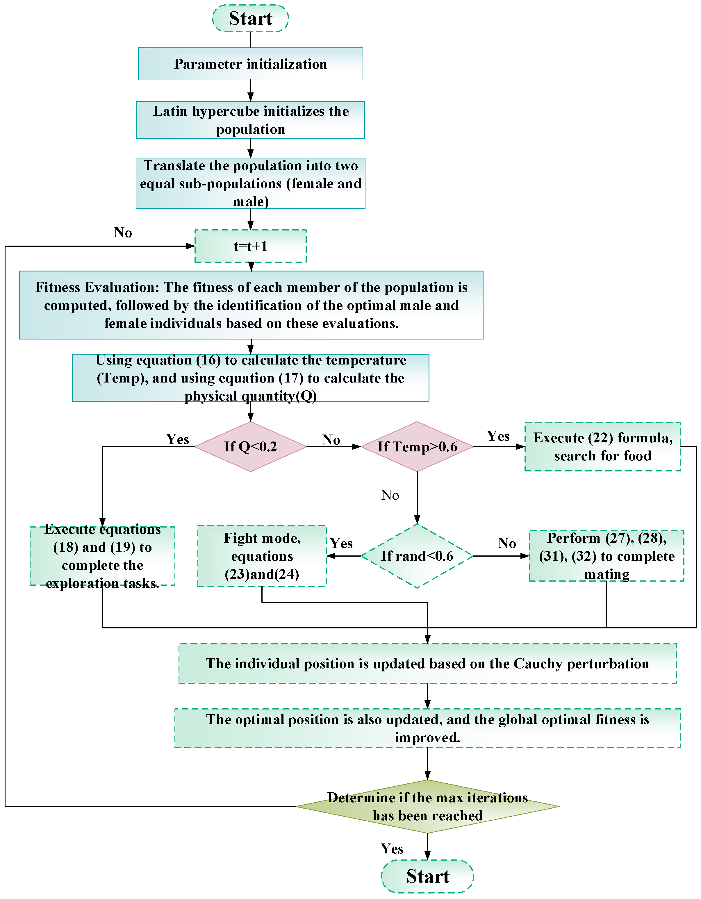
To sum up, Figure 4 illustrates the flow chart of the enhanced SO algorithm.

Step 1 (Initialization): The algorithm’s key control parameters are established, including the population size (N), the maximum number of iterations (T), the search space boundaries ([lb, ub]), and the problem’s dimensionality (dim).

Step 2: Employ LHS to initialize the population and produce the initial solution.

Step 3: Based on Equations (14) and (15), the population is divided into two groups, a fitness function is created, corresponding fitness values are computed, and the optimal individuals (best men and women) are identified.

Step 4: The algorithm begins this stage by computing two key control parameters: the ambient temperature and the food quantity (Q), via the formulations in Equations (16) and (17), respectively.

Step 5: Subsequently, the value of Q serves as a conditional determinant for the algorithm’s next phase. If Q falls below a predefined threshold, the algorithm transitions into an exploration-focused foraging mode, wherein the position vectors of the population members are updated according to the mathematical models presented in Equations (18) and (20). Otherwise, the algorithm enters an exploitation phase involving combat and mating.

Step 6: If food is sufficient and (Temp > 0.6), simply forage and consume the current food, updating the position as indicated in Equation (22).

Step 7: Decide if it wants to go into combat or mating mode based on the random number Rand. If the snake is in combat mode, update its location with Equations (23) and (26); if it is in mating mode, use Equations (27) and (28) to update its location. After mating and hatching, select the worst and replace them.

Step 8: Update the current fitness values of each individual based on the t-distribution mutation strategy, and update the global optimal fitness value.

Step 9: Check if it has reached the maximum number of iterations. If not, proceed to the next iteration; otherwise, finish the iteration and output the fitness and location of the best individual.

Step 10: Adaptive perturbation is applied to the optimum person in accordance with Equation (35). If the mutation is superior to the original, output the location and optimum fitness value of the mutant. Otherwise, output the location and optimum fitness.

2.6. The Development of a Transmission Line Icing Forecast Model Based on ISO-DHKELM

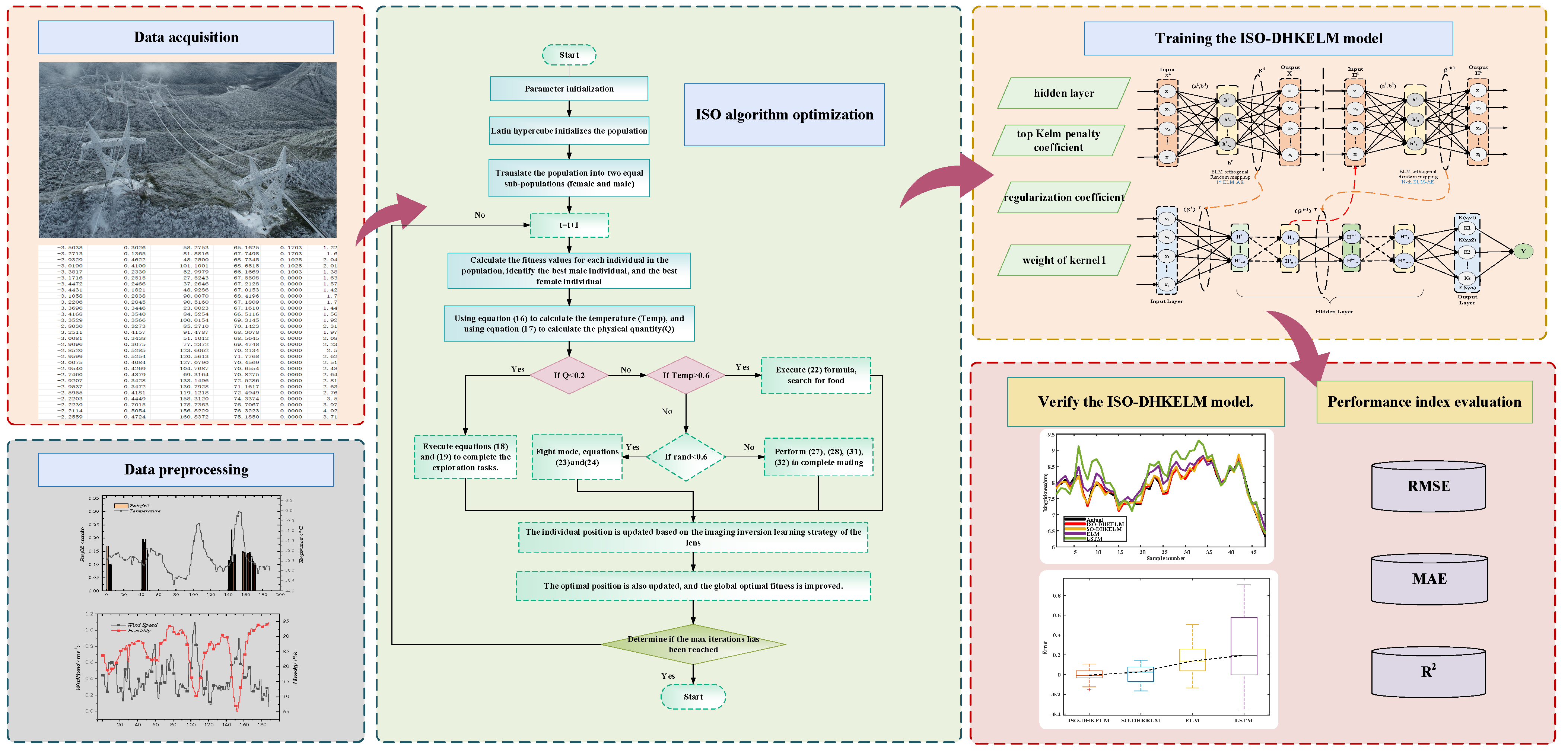
Figure 5 illustrates the prediction process of the ISO-DHKELM model.

(1)

Data sample acquisition: Collect data samples necessary for predicting transmission line icing thickness, including meteorological and environmental variables.

(2)

Data normalization: Normalize the collected data to a standard range [0–1] to enhance model efficiency and stability.

(3)

ISO algorithm initialization: Set initial parameters for the ISO algorithm, including population size and snake positions.

(4)

Position update of snakes: Use the ISO algorithm’s position update strategy to iteratively adjust snake positions for optimal solution search.

(5)

Hyperparameter optimization: Optimize DHKELM model hyperparameters using the ISO algorithm to improve prediction accuracy.

(6)

Icing thickness prediction: Apply the trained ISO-DHKELM model to predict transmission line icing thickness.

(7)

Performance evaluation: Evaluate the model’s prediction performance using metrics like MAE, RMSE, and R² to validate its effectiveness.

3. Data Processing and Analysis

3.1. Principle of Grey Relational Analysis

Grey relational analysis is employed to study uncertain systems. It judges the correlation by comparing the similarity of data curves. The steps include data collection, processing, modeling, validation, and application, and it is widely used in many fields. The principle is to calculate the correlation coefficient between the parent series and the child series. The higher the coefficient, the more significant the correlation.

The calculation process of the grey relational analysis method is as follows:

(1)

Determine the sequence for analysis: Based on the analysis object, the ice thickness of the power line is determined as the reference sequence for grey relational analysis, as shown in Equation (36):

$$\begin{array}{c}{X}_0=\left\{X_0\left(1\right),X_0\left(2\right),{\dots ,X}_0\left(k\right)\right\}\end{array}$$

(36)

The various factors affecting the ice thickness are used as the comparison sub-sequences, as shown in Equation (37):

$$\begin{array}{c}\left\{\begin{array}{c}{X}_1=\left\{X_1\left(1\right),X_1\left(2\right),{\dots ,X}_1\left(k\right)\right\}\\ \dots \dots \\ X_m=\left\{X_m\left(1\right),X_m\left(2\right),{\dots ,X}_m\left(k\right)\right\}\end{array}\right.\end{array}$$

(37)

In the formula, $X_0$ is the data of the line icing thickness after standardization, $X_i$ represents the data of other micro-meteorological factors after standardization.

(2)

Normalize data: Normalize selected sequences to eliminate dimensional differences before correlation analysis, as shown in Equation (38):

$$\begin{array}{c}{x}_i^{\prime }={\displaystyle \frac{x_i-x_{min}}{x_{max}-x_{min}}}\end{array}$$

(38)

In the formula:$x_i$ represents the original value, $x_{min}$ and $x_{max}$ represent the minimum and maximum values, respectively.

(3)

Calculate the correlation coefficient between the parent sequence and each sub-sequence using the formula in Equation (39):

$$\begin{array}{c}{\xi }_i\left(k=\right){\displaystyle \frac{{min}_i{min}_k\left|X_0\left(k\right)-X_i\left(k\right)\right|+\eta {max}_i{max}_k\left|X_0\left(k\right)-X_i\left(k\right)\right|}{\left|X_0\left(k\right)-X_i\left(k\right)\right|+\eta {max}_i{max}_k\left|X_0\left(k\right)-X_i\left(k\right)\right|}}\end{array}$$

(39)

In the formula, $\eta$ shows the correlation strength between parent and sub-sequence. It’s non-negative, with optimal discrimination when $\eta$ ∈ [0.321, 0.588]. Usually, $\eta$ = 0.5.

(4)

Calculate the degree of correlation: Calculate the correlation degree between the reference sequence and factors. The correlation coefficient shows a sub-sequence relation to the parent sequence. Scattered correlation values over time need integration for easier comparison, resulting in the grey relational degree. The formula is as follows:

$$\begin{array}{c}{r}_i={\displaystyle \frac{1}{n}}{\displaystyle \sum _{k=1}^n}{\epsilon }_i\left(k\right),k=\mathrm{1,2},3,\dots n\end{array}$$

(40)

(5)

Correlation degree ranking: Based on calculated results, the relationship between sequences is ranked. Higher values indicate closer relationships, while lower values indicate weaker relationships.

3.2. Grey Correlation Analysis Example

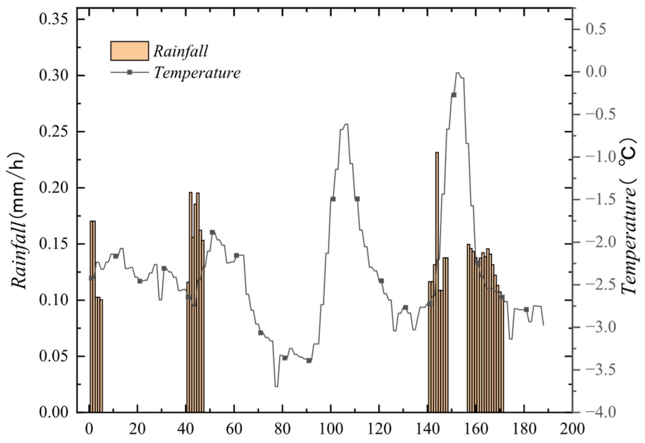
The formation of transmission line icing is an inherently complex phenomenon. Consequently, selecting input variables based on operational conditions can result in a high-dimensional feature space, which may increase the model’s computational burden, thereby reducing training efficiency and extending the required learning duration. Conversely, if the number of input variables is excessively reduced, it may compromise the model’s prediction accuracy. To address this, the grey correlation analysis method is employed to pinpoint the key factors that impact the ice thickness on conductors [33]. The analysis is based on historical ice monitoring data from the “Kangshu No. 2 line” transmission line in Sichuan. The icing growth period spanned from 11:00 on 22 January 2024 to 08:00 on 26 January 2024, with data collected at 30-min intervals, yielding a total of 188 data sets.

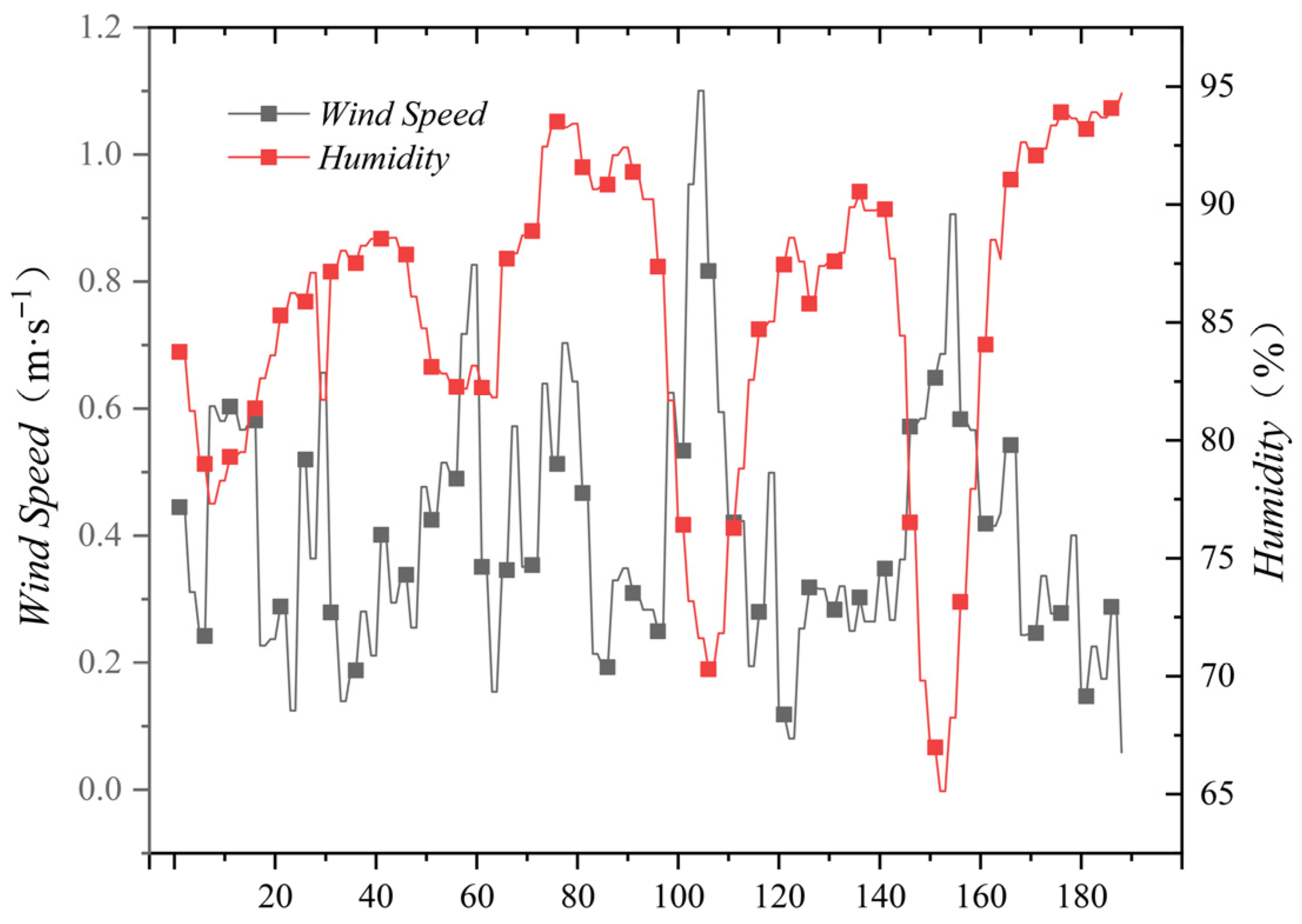
The development of ice thickness on transmission lines is closely related to the surrounding meteorological environment. The formation of conductor icing generally should meet the following meteorological conditions: the meteorological conditions for icing formation are usually temperatures below 0 degrees Celsius, a certain wind speed, and atmospheric humidity reaching above 80% with a certain amount of rainfall. The melting and shedding of line icing typically occur under the conditions of increased ambient temperature and increased ambient wind speed. As mentioned earlier, the original data sequence charts for temperature, wind speed, air humidity, and rainfall are shown in Figure 6 and Figure 7:

There is a close relationship between the formation of ice accumulation and the weather conditions in the vicinity. Based on the historical monitoring data shown in the figure, the meteorological conditions for ice formation typically occur when the temperature is below 0 degrees Celsius, with a certain wind speed and atmospheric humidity reaching above 80%, and there is a certain amount of rainfall. The melting and shedding of line ice usually occur under conditions of rising environmental temperature and increasing environmental wind speed.

Due to the difficulty in ensuring the real-time nature and consistency of historical data on line icing and environmental meteorological data, it is impossible to determine the exact relationship between the two based on manual observation. Therefore, a grey relational analysis was conducted between them, and the correlation between line icing thickness and other influencing factors is given in

Table 2. The degree of correlation between each influencing factor and ice thickness.

Influencing Factors	Temperature	Wind Speed	Wind Direction	Humidity	Rainfall	Atmospheric Pressure
Relevance	0.6519	0.5841	0.5481	0.6250	0.5257	0.4991

as follows:

When the correlation coefficient falls below 0.5, the correlation is deemed to be weak; when the correlation coefficient ranges from 0.5 to 1, the correlation is regarded as strong. As indicated in Table 1, the ranking of correlation strength is as follows: temperature > humidity > wind speed > wind direction > rainfall > air pressure. In particular, environmental temperature exhibits the highest correlation coefficient, suggesting a significant relationship between temperature and ice accretion prediction. Air pressure, which ranks last, has a correlation coefficient less than 0.5 and is considered to have a weak correlation.

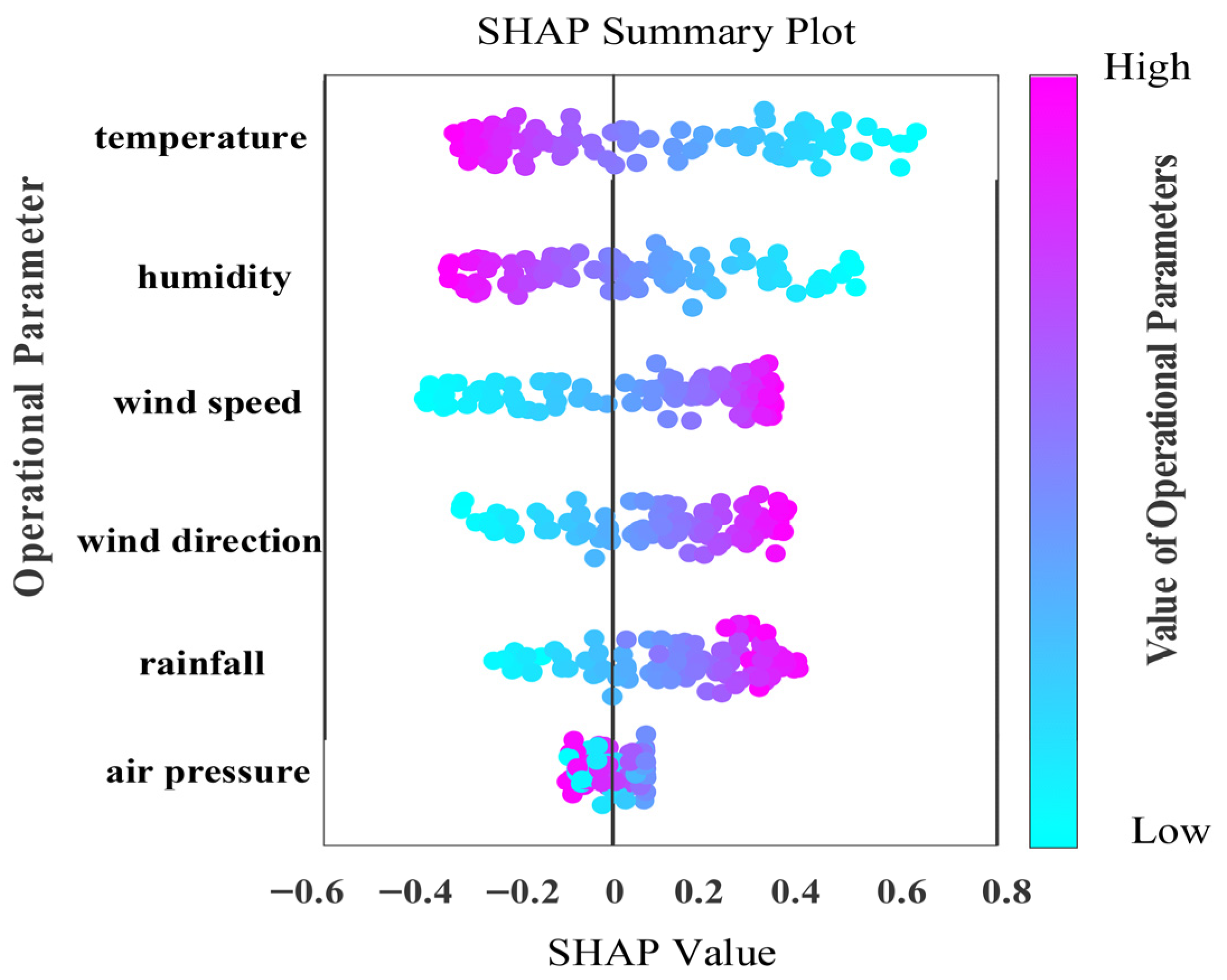
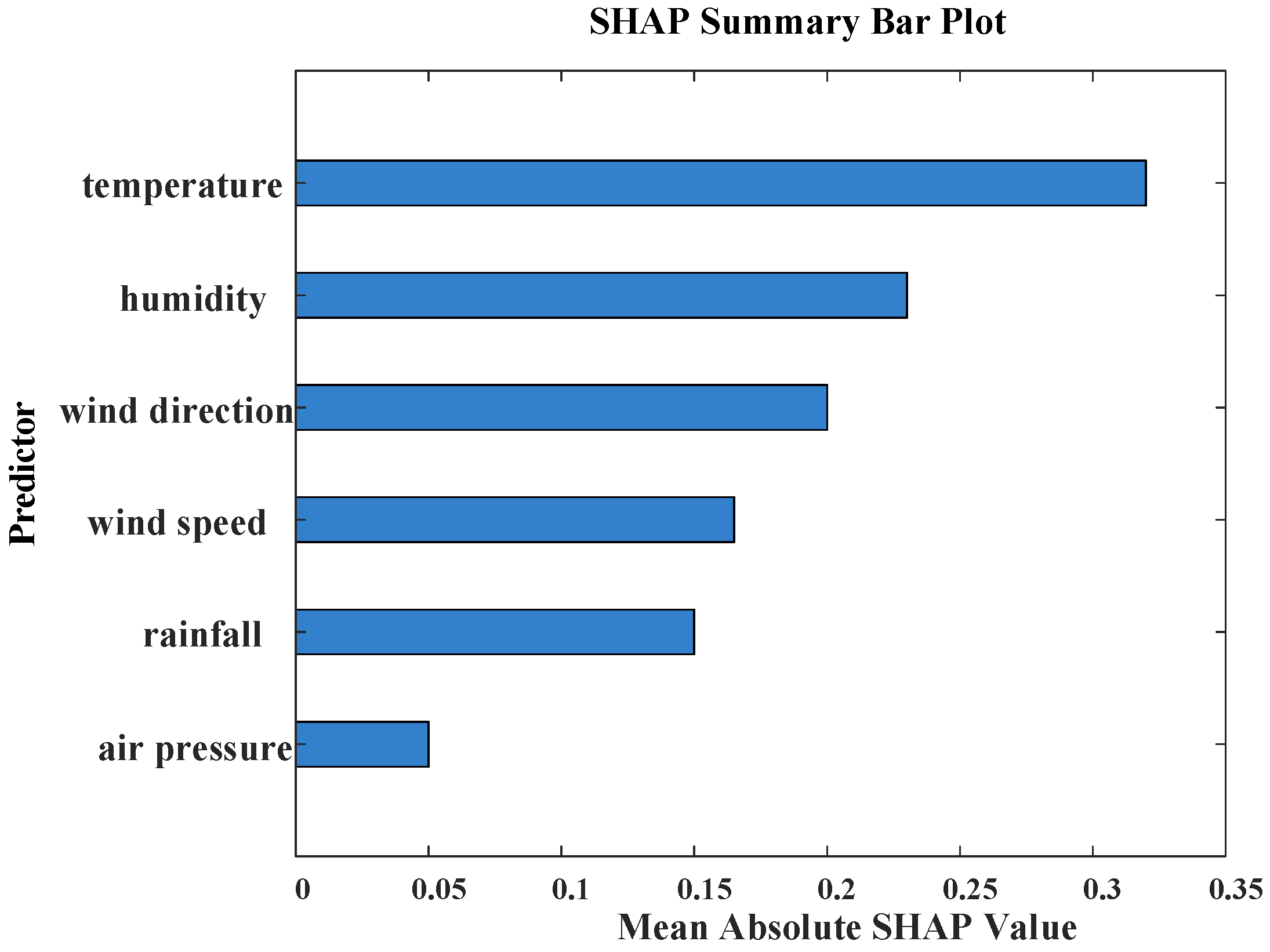
To further verify the validity of the input features, this study employs the Shapley additive explanation (SHAP) interpretability framework [34]. SHAP adopts an additive attribution strategy to compute each input variable’s marginal contribution to the model’s output, thereby quantifying the relative importance of all features at the global level. For any single sample, its SHAP value represents the exact quantitative impact of that feature on the corresponding prediction. As shown in Figure 8 and Figure 9, SHAP is employed to interpret the characteristics of input for DHKELM, with features ranked in descending order of importance based on mean absolute SHAP values. Positive SHAP values correspond to positive effects, while negative values correspond to negative effects. The color bar in Figure 8 illustrates that a color closer to the upper end represents a higher feature value, while a color nearer to the lower end corresponds to a smaller feature value. Furthermore, a wider color bar reflects a more significant feature impact, suggesting that such a feature is more critical.

As shown in Figure 8, the variables are ranked by contribution as follows: temperature, humidity, wind speed, wind direction, precipitation, and atmospheric pressure. Figure 9 further confirms that temperature, humidity, and wind speed have the largest mean absolute SHAP values. Integrating the results of grey relational analysis and SHAP, this paper ultimately selects temperature, humidity, wind speed, wind direction, and precipitation as the input variables for the predictive model.

4. Simulation Case Analysis

The experiments were conducted on the MATLAB 2022b platform, with the following hardware specifications: an Intel Core i7-14650HX 2.20 GHz central processing unit (CPU), 16 GB of random-access memory (RAM), and a 64-bit Windows operating system.

4.1. Optimizer Performance Analysis

In this section, to verify the rationality and reliability of the optimization strategy selection of the ISO algorithm, six benchmark test functions were chosen to evaluate the performance of the ISO algorithm, as shown in

Table 3. Test function.

Function	Dimension	Range
$f_1\left(\mathrm{x}\right)={\displaystyle \sum _{i=1}^{30}}{x}_i^2$	30	[−100, 100]
$f_2\left(\mathrm{x}\right)={\displaystyle \sum _{i=1}^{30}}\left|x_i\right|+{\displaystyle \prod _{i=1}^{30}}\left|x_i\right|$	30	[−10, 10]
$f_3\left(\mathrm{x}\right)={\displaystyle \sum _{i=1}^{30}}{\left({\displaystyle \sum _{j=1}^i}{x}_j\right)}^2$	30	[−100, 100]
$f_4\left(\mathrm{x}\right)={\displaystyle \sum _{i=1}^{30}}\left[x_i^2-10cos\left(2\pi x_i\right)+10\right]$	30	[−5.12, 5.12]
$f_5\left(\mathrm{x}\right)=-20exp\left(-0.2\sqrt{{\displaystyle \frac{1}{30}}{\displaystyle \sum _{i=1}^{30}}{x}_i^2}\right)-exp\left({\displaystyle \frac{1}{30}}{\displaystyle \sum _{i=1}^{30}}cos\left(2\pi x_i\right)\right)+20+e$	30	[−32, 32]
$f_6\left(\mathrm{x}\right)={\displaystyle \sum _{i=1}^{11}}{\left[a_i-{\displaystyle \frac{x_1\left(b_i^2+b_i{x}_2\right)}{b_i^2+b_i{x}_3+x_4}}\right]}^2$	30	[−5, 5]

. Among the six test functions, $f_1\left(\mathrm{x}\right)-f_3\left(\mathrm{x}\right)$ are unimodal test functions used to examine the convergence ability and solution accuracy of the algorithm; $f_4\left(\mathrm{x}\right)-f_6\left(\mathrm{x}\right)$ are multimodal test functions that can effectively test the global performance of the algorithm.

To comprehensively verify the effectiveness of the ISO algorithm proposed in this paper, we selected the PSO algorithm, WOA algorithm, and SO algorithm for comparison. These algorithms have been proven to have good optimization capabilities. To accurately evaluate the performance of the ISO algorithm and the comparison algorithms, all algorithms have a unified population size of 30 and a maximum iteration count of 500. Each algorithm was independently executed 20 times. Table 3 shows the experimental results.

Table 4. Test results.

Function	Algorithms	Average	Worst Value	Optimal
	ISO	0	0	0
	SO	4.9393 × 10−99	0	2.3053 × 10−99
$f\left(1\right)$	GWO	4.2078 × 10−57	1.2424 × 10−75	5.8831 × 10−49
	PSO	2.5409 × 10−75	2.4676 × 10−25	7.9196 × 10−29
	ISO	0	0	0
	SO	2.9202 × 10−99	7.7955 × 10−99	2.6854 × 10−78
$f\left(2\right)$	GWO	8.4728 × 10−56	5.5396 × 10−39	1.2043 × 10−69
	PSO	3.6561 × 10−60	2.4854 × 10−42	1.3293 × 10−24
	ISO	0	0	0
	SO	7.7994 × 10−49	2.4663 × 10−42	3.9772 × 10−9
$f\left(3\right)$	GWO	9.9272 × 10−17	2.7574 × 10−99	2.8674 × 10−35
	PSO	2.2384 × 10−15	4.2198 × 10−65	606.74 × 10−60
	ISO	0	0	0
	SO	0	0	0
$f\left(4\right)$	GWO	1.5218	2.7839	0
	PSO	49.8859	9.6766	34.4649
	ISO	4.4409 × 10−10	0	4.4409 × 10−20
	SO	4.4409 × 10−4	0	4.4409 × 10−16
$f\left(5\right)$	GWO	0.0134	1.9036 × 10−21	7.8604 × 10−14
	PSO	0.4163	0.0436	0.0786
	ISO	7.0024 × 10−94	0	4.9407 × 10−99
	SO	4.9393 × 10−51	0	2.3053 × 10−61
$f\left(6\right)$	GWO	4.2078 × 10−27	1.2424 × 10−26	5.8831 × 10−29
	PSO	0.25409	0.24676	0.079196

shows that ISO has a significant performance advantage for unimodal test functions, achieving the theoretical optimum and far outperforming SO and other comparison algorithms. Furthermore, compared with the three algorithms, ISO has the smallest standard deviation, indicating that ISO has the best exploration capability and stability. For multimodal test functions, ISO still has the highest search accuracy compared with other algorithms. The results show that ISO has strong global search capability and local optimum avoidance capability, as well as high optimization stability.

4.2. Model Performance Assessment Metric

In order to verify the excellent performance of the model, the root mean square error (RMSE), mean absolute error (MAE), and coefficient of determination (R²) are employed as indices to verify the modeling accuracy.

$$\begin{array}{c}RMSE=\sqrt{{\displaystyle \frac{1}{n}}{\displaystyle \sum _{i=1}^n}\left(f\right(x_i)-y_i{)}^2}\end{array}$$

(41)

$$\begin{array}{c}MAE={\displaystyle \frac{1}{n}}{\displaystyle \sum _{i=1}^n}\left|f\left(x_i\right)-y_i\right|\end{array}$$

(42)

$$\begin{array}{c}{R}^2=1-{\displaystyle \frac{\sum _i{\left(f\right(x_i)-y_i)}^2}{\sum _i{(f\left(x_i\right)-\overline{y})}^2}}\end{array}$$

(43)

where, n indicates the number of samples; $f\left(x_i\right)$ signifies the actual value; $y_i$ represents the forecast value; $\overline{y}$ denotes the mean value.

4.3. Impact of Different Input-Feature Combinations on Model Performance and Verification

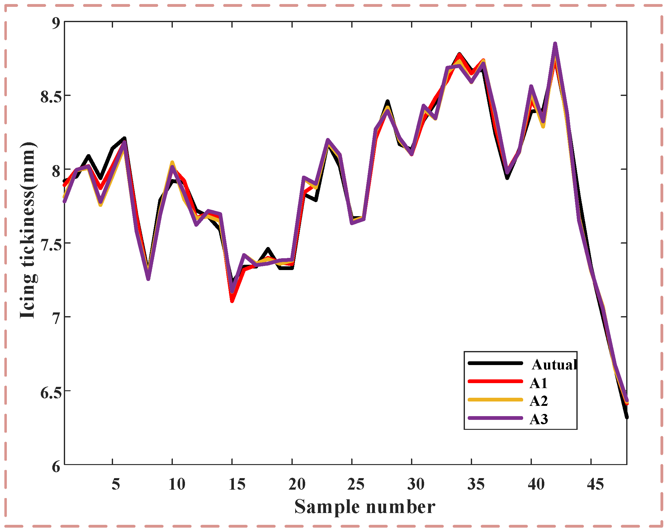
High-frequency features are the key determinants for predicting ice thickness, and different feature combinations have significant impacts on prediction accuracy. Literature [35] selects temperature, humidity, and conductor tension as model inputs, while Literature [36] uses temperature, humidity, wind speed, and wind direction as inputs for the ice prediction model. To verify the superiority of the features extracted in this study, under the premise of fixing all hyperparameters, we systematically adjust the input channels to retrain the DHKELM model and conduct a comparative analysis between the feature set in this paper and those used in the aforementioned literature (denoted as A1, A2, and A3, respectively).

Figure 10 and

Table 5. Performance metrics of prediction results with different feature combinations.

Feature Combination	RMSE	MAE	R2
A1	0.057	0.044	0.993
A2	0.080	0.066	0.977
A3	0.086	0.074	0.973

clearly show the ice thickness prediction results for three different feature combinations. Among the three scenarios, the feature combination proposed in this paper achieves the highest goodness-of-fit as well as the lowest RMSE and MAE. This indicates that the constructed input feature combination enables the model to predict ice coating thickness more accurately, effectively improving the precision and generalization ability of ice thickness prediction.

4.4. Case Studies

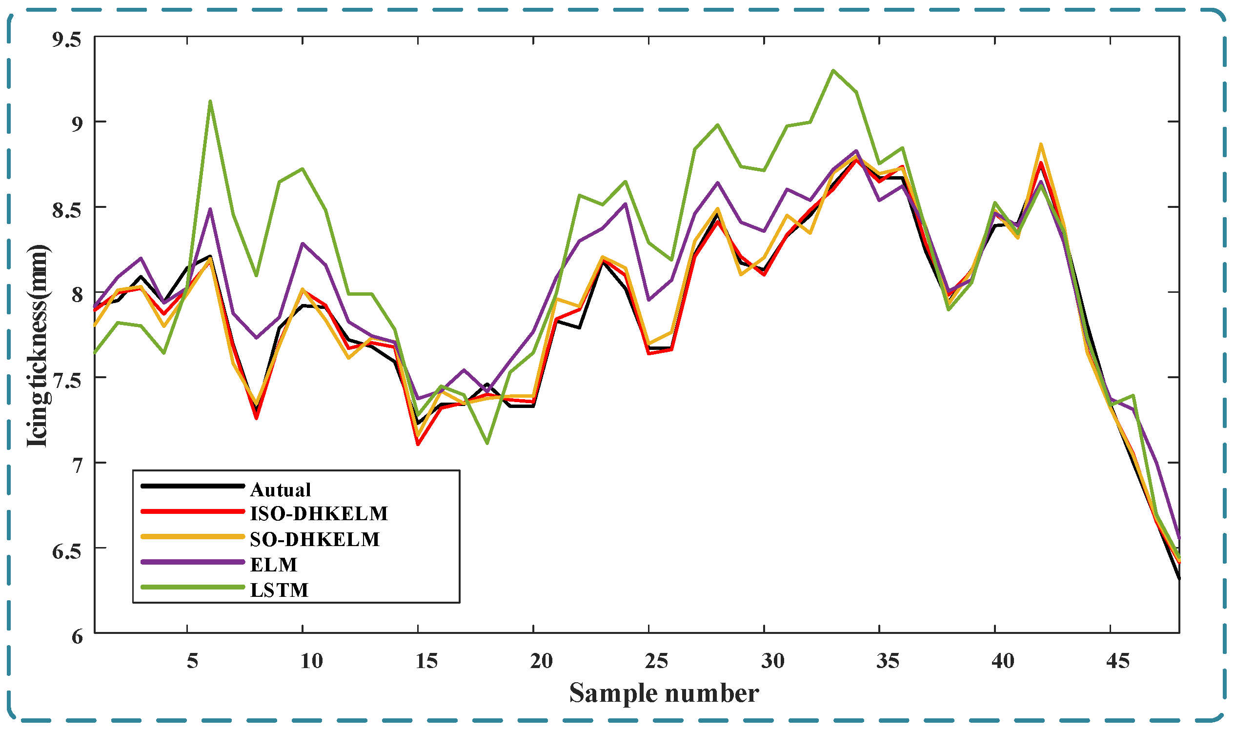
For a comprehensive performance evaluation, the proposed ISO-DHKELM algorithm was benchmarked against three other predictive methodologies: SO-DHKELM, ELM, and LSTM. To ensure a fair and consistent comparison, the dataset was partitioned chronologically, with the initial 140 samples constituting the training set and the subsequent 48 samples forming the testing set. Figure 11 illustrates a comparison between the predicted values of transmission line icing thickness generated by four different algorithms and the actual values. In this figure, the horizontal axis denotes the sample number, while the vertical axis indicates the icing thickness in millimeters. As depicted in the figure, the ISO-DHKELM model introduced in this paper demonstrates the most accurate fitting performance among the compared models. In contrast, the LSTM neural network exhibits a notable deviation from the expected values. Additionally, the SO-DHKELM model is capable of optimizing the parameter selection for DHKELM, which effectively minimizes the model error. However, the conventional SO algorithm tends to become trapped in local optima, which hampers its ability to produce optimal parameters and consequently restricts the model’s precision. Concurrently, the standard ELM model, which is defined by its simple architecture and reliance on randomly initialized weights, exhibits significant deviations between its predictions and the observed data. This often results in substantial prediction errors and a progressive divergence from the true values. In summary, the ISO-DHKELM algorithm performs well in predicting the thickness of transmission line icing, especially in handling data fluctuations with higher precision.

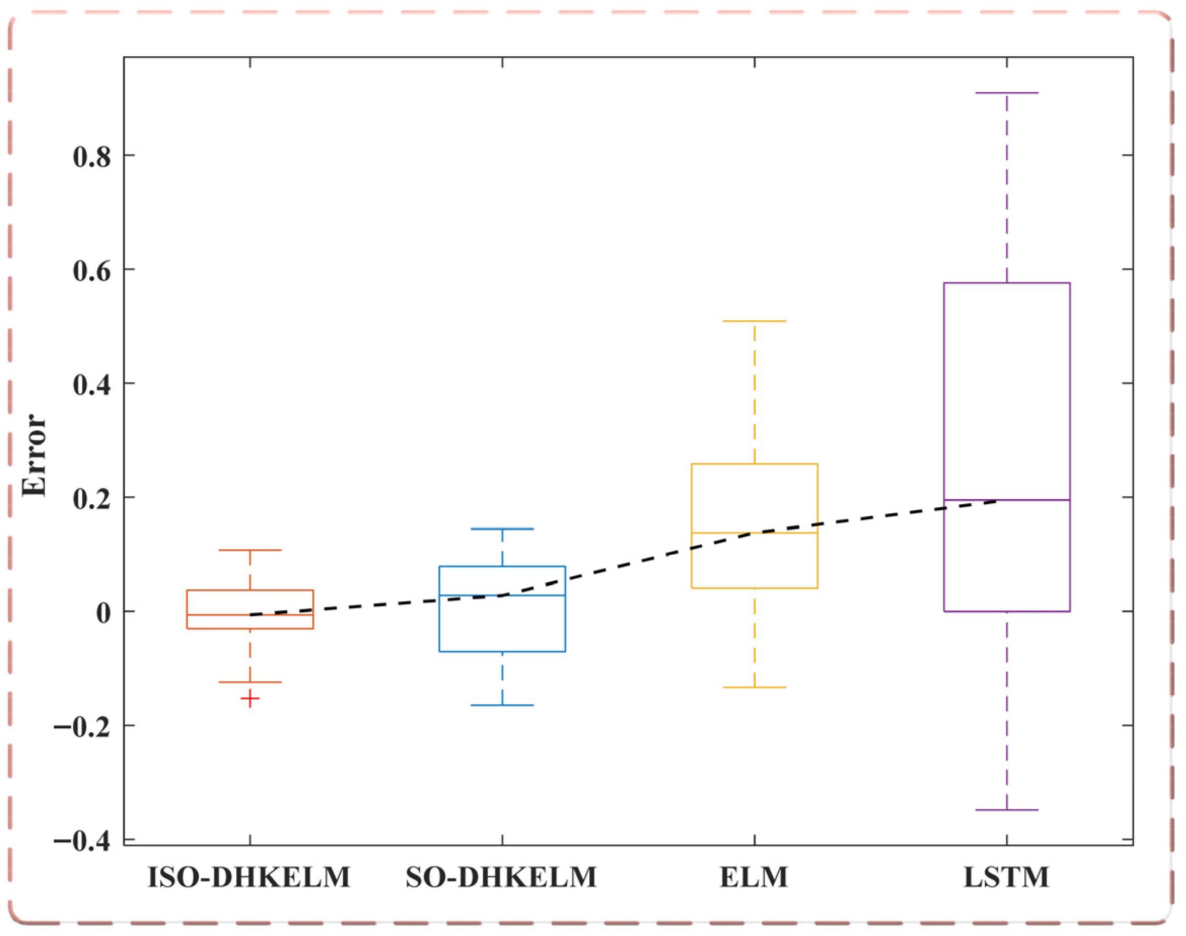
Figure 12: The distribution of prediction errors for the four evaluated model configurations is visualized using box plots. This representation intuitively elucidates the distinct error characteristics inherent to each model for the task of transmission line ice thickness prediction. As depicted in the figure, the LSTM and ELM models exhibit significant fluctuations in prediction errors and considerable dispersion in prediction results. This indicates that these two models need to improve their prediction stability when dealing with the complex task of ice coverage prediction on transmission lines. While the SO-DHKELM model demonstrates a discernible improvement in overall predictive performance and a reduction in error magnitude, the proposed ISO-DHKELM model exhibits a markedly superior level of prediction accuracy. The prediction errors of the ISO-DHKELM model are mostly concentrated within an interval of 0.1, which fully demonstrates the high accuracy and strong stability of this model in the scenario of ice coverage prediction on transmission lines.

As can be seen from

Table 6. Comparison of prediction errors and computational time of four models.

Prediction Model	RMSE	MAE	R2	Operation Time(s)
ISO-DHKELM	0.057	0.044	0.993	7.8
SO-DHKELM	0.086	0.075	0.973	8.1
ELM	0.223	0.179	0.819	6.5
LSTM	0.438	0.347	0.303	30

, it is evident that the application of the SO and ISO algorithms to optimize the DHKELM model has led to a significant enhancement in its ability to predict ice thickness. Specifically, the ISO-DHKELM model stands out as the most effective among all the models evaluated, as it achieves the lowest error values across all metrics. For this superior model, the RMSE is recorded at 0.057, the MAE is 0.044, and the R² reaches an impressive 0.993. In terms of operation time, although the training time of the model proposed in this paper is not the fastest, it achieves the highest accuracy within a relatively fast running time and can also meet the needs of real-time applications. These results clearly indicate that compared with other methods, the ISO-DHKELM method has higher accuracy and applicability in ice thickness prediction.

4.5. Comparison with Existing Approaches

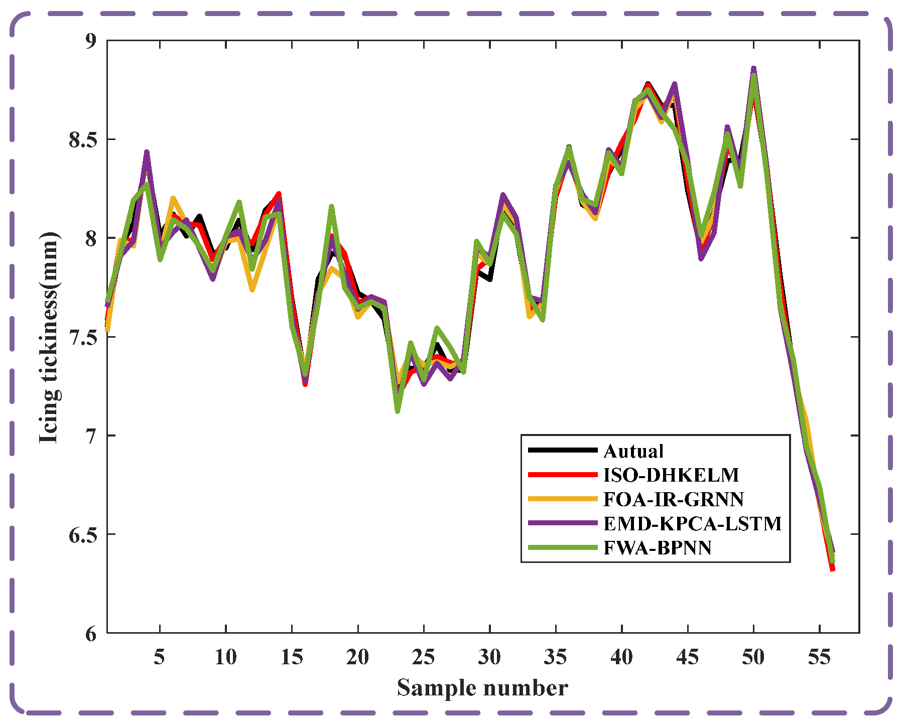
To objectively and quantitatively evaluate the accuracy and generalization capability of the proposed model, we conducted a comprehensive comparative analysis against current mainstream and state-of-the-art icing thickness prediction models under the same benchmark, using identical datasets and evaluation metrics. The detailed comparison results are shown in Figure 13.

As can be seen from the comparative experimental results in

Table 7. Comparison of prediction errors and operation time of four models.

Prediction Model	RMSE	MAE	R2	Operation Time(s)
ISO-DHKELM	0.046	0.037	0.991	7.9
FOA-IR-GRNN	0.083	0.070	0.971	13.5
EMID-KPCA-LSTM	0.085	0.075	0.970	65
FWA-BPNN	0.095	0.081	0.963	50

, the proposed ISO-DHKELM model demonstrates outstanding comprehensive performance in the task of transmission line icing prediction. On the test set, the model achieved the lowest RMSE and MAE, along with the highest R², significantly outperforming existing research methods. It is particularly noteworthy that while achieving optimal prediction accuracy, ISO-DHKELM also incurs lower computational cost compared to other benchmark algorithms, highlighting the efficiency and superiority of integrating the ISO algorithm with the DHKELM model.

5. Conclusions

In recent years, extreme weather events have increased, and ice disasters have become a major threat to the power grid as ultra-high voltage lines expand. These disasters can cause widespread blackouts by damaging lines and towers. Therefore, it is essential to study and predict transmission line ice thickness from a micrometeorological perspective.

Based on historical icing data, this paper first elucidates the physical mechanisms underlying ice accretion. It then employs statistical methods to analyze the correlation between key influencing factors and icing severity. Furthermore, the study conducts a comparative evaluation of multiple machine learning models and proposes an enhanced SO algorithm to optimize the DHKELM:

(1)

Research method and input variable selection: Grey relational analysis was employed to quantify the correlation between transmission-line ice thickness and meteorological variables, and the findings were cross-validated with SHAP analysis to select the strongly correlated factors as model inputs.

(2)

Model construction and optimization: A transmission line icing prediction model, ISO-DHKELM, based on the ISO algorithm for optimizing the DHKELM, was proposed, and the ISO algorithm was used to optimize the key parameters of the DHKELM model.

(3)

Model validation and result analysis: Through simulation and comparison with actual icing cases, compared with SO-DHKELM, ELM, and LSTM, ISO-DHKELM, respectively, reduced RMSE by 2.9%, 16.6%, and 38.1%, MAE by 3.1%, 13.5%, and 30.3%, and increased R² by 2%, 17.4%, and 69% on the validation set.

Although this paper has achieved some results, there are still shortcomings. Future research can be further conducted in the following aspects:

(1)

The paper only considers the icing condition under ideal conditions. In the future, the impact of line shape on the icing mechanism can be studied and the model can be improved accordingly.

(2)

The model in this paper solely focuses on meteorological factors. In the future, other icing influencing factors, such as topography, need to be comprehensively considered.

References

1. Farzaneh, M.; Baker, C.; Bernstorf, A.; Brown, K.; Chisholm, W.; de Tourreil, C.; Drapeau, J.; Fikke, S.; George, J.; Gnandt, E.; et al. Insulator icing test methods and procedures: A position paper prepared by the IEEE task force on insulator icing test methods. IEEE Trans. Power Deliv. 2003, 18, 1503–1515. [Google Scholar] [CrossRef]
2. Richardson, A.S. Dynamic analysis of lightly iced conductor galloping in two degrees of freedom. IEEE Proc. C Gener. Transm. Distrib. 1981, 128, 211–218. [Google Scholar] [CrossRef]
3. Gade Herman, G. Melting of Ice in Sea Water: A primitive model with application to the antarctic ice shelf and icebergs. J. Phys. Oceanogr. 2010, 9, 189–198. [Google Scholar] [CrossRef]
4. Chang, S.E.; Mcdaniels, T.L.; Mikawoz, J.; Peterson, K. Infrastructure failure interdependencies in extreme events: Power outage consequences in the 1998 Ice Storm. Nat. Hazards 2007, 41, 337–358. [Google Scholar] [CrossRef]
5. Bin, F.L.G.; Rong, Z.F.; Gang, L.; Hong, Y.; Chao, Q.G.; Liangchi, S.; En, Y.; Xiang, L. A Research of Drawing and Application of Distribution Diagram of Yunnan Ice Region Based on The Typical Ice Model of Low Latitude Plateau Area. In Proceedings of the 2018 International Conference on Power System Technology (POWERCON), Guangzhou, China, 6–8 November 2018. [Google Scholar] [CrossRef]
6. Wigley, T.M.L.; Briffa, K.R.; Jones, P.D. Modeling of ice accretion on wires. J. Appl. Meteorol. 1984, 23, 929–939. [Google Scholar] [CrossRef]
7. Liao, Y.; Duan, L. Study on Estimation Model of Wire Icing Thickness in Hunan Province. Trans. Atmos. Sci. 2010, 33, 395–400. [Google Scholar] [CrossRef]
8. Li, P.; Zhao, N.; Zhou, D.; Cao, M.; Li, J.; Shi, X. Multivariable time series prediction for the icing process on overhead power transmission line. Sci. World J. 2014, 2014, 256815. [Google Scholar] [CrossRef] [PubMed]
9. Sirui, Y.; Mengjie, S.; Runmiao, G.; Jiwoong, B.; Xuan, Z.; Shiqiang, Z. A review of icing prediction techniques for four typical surfaces in low-temperature natural environments. Appl. Therm. Eng. 2024, 241, 122418. [Google Scholar] [CrossRef]
10. Li, P.; Li, N.; Li, Q.M.; Cao, M.; Chen, H.X. Prediction Model for Power Transmission Line Icing Load Based on Data-Driven. Adv. Mater. Res. 2011, 143–144, 1295–1299. [Google Scholar] [CrossRef]
11. Chen, Y.; Li, P.; Ren, W.; Shen, X.; Cao, M. Field data–driven online prediction model for icing load on power transmission lines. Meas. Control. 2020, 53, 126–140. [Google Scholar] [CrossRef]
12. Kong, F.; Song, G.P. Middle long power load forecasting based on dynamic grey prediction and support vector machine. Int. J. Adv. Comput. Technol. 2012, 4, 148–156. [Google Scholar] [CrossRef]
13. Li, Q.; Li, P.; Zhang, Q.; Ren, W.; Cao, M.; Gao, S. Icing load prediction for overhead power lines based on SVM. In Proceedings of the 2011 International Conference on Modelling, Identification and Control, Shanghai, China, 26–29 June 2011. [Google Scholar] [CrossRef]
14. Chen, S.; Dai, D.; Huang, X.; Sun, M. Short-Term Prediction for Transmission Lines Icing Based on BP Neural Network. In Proceedings of the 2012 Asia-Pacific Power and Energy Engineering Conference, Shanghai, China, 27–29 March 2012. [Google Scholar] [CrossRef]
15. Wang, W.; Zhao, D.; Fan, L.; Jia, Y. Study on Icing Prediction of Power Transmission Lines Based on Ensemble Empirical Mode Decomposition and Feature Selection Optimized Extreme Learning Machine. Energies 2019, 12, 2163. [Google Scholar] [CrossRef]
16. Niu, D.; Wang, H.; Chen, H.; Liang, Y. The General Regression Neural Network Based on the Fruit Fly Optimization Algorithm and the Data Inconsistency Rate for Transmission Line Icing Prediction. Energies 2017, 10, 2066. [Google Scholar] [CrossRef]
17. Liang, Y.; Yao, D.; Gao, Y.; Jiang, K. PSO-CGAN-Based Iced Transmission Line Galloping Prediction Method. IEICE Trans. Fundam. Electron. Commun. Comput. Sci. 2025, E108.A, 53–64. [Google Scholar] [CrossRef]
18. Xu, X.; Niu, D.; Wang, P.; Lu, Y.; Xia, H. The Weighted Support Vector Machine Based on Hybrid Swarm Intelligence Optimization for Icing Prediction of Transmission Line. Math. Probl. Eng. 2015, 2015, 1–9. [Google Scholar] [CrossRef]
19. Ma, T.; Niu, D. Icing Forecasting of High Voltage Transmission Line Using Weighted Least Square Support Vector Machine with Fireworks Algorithm for Feature Selection. Appl. Sci. 2016, 6, 438. [Google Scholar] [CrossRef]
20. Ma, T.; Niu, D.; Fu, M. Icing Forecasting for Power Transmission Lines Based on a Wavelet Support Vector Machine Optimized by a Quantum Fireworks Algorithm. Appl. Sci. 2016, 6, 54. [Google Scholar] [CrossRef]
21. Wang, Y.; Zhao, K.; Hao, Y.; Yao, Y. Short-term wind power prediction using a novel model based on butterfly optimization algorithm-variational mode decomposition-long short-term memory. Appl. Energy 2024, 366, 123313. [Google Scholar] [CrossRef]
22. Yang, H.; Xu, W.; Zhao, J.; Wang, D.; Dong, Z. Predicting the probability of ice storm damages to electricity transmission facilities based on ELM and Copula function. Neurocomputing 2011, 74, 2573–2581. [Google Scholar] [CrossRef]
23. Gu, H.; Zhang, Q.; Wang, L. An intelligent method for fault situation in double-circuit transmission lines utilizing extreme learning machine. Electr. Eng. 2025, 107, 2051–2062. [Google Scholar] [CrossRef]
24. Mo, D.; Wang, S.; Fan, Y.; Takyi-Aninakwa, P.; Zhang, M.; Wang, Y.; Fernandez, C. Enhanced multi-constraint dung beetle optimization-kernel extreme learning machine for lithium-ion battery state of health estimation with adaptive enhancement ability. Energy 2024, 307, 132723. [Google Scholar] [CrossRef]
25. Hashim, F.A.; Hussien, A.G. Snake optimizer: A novel meta-heuristic optimization algorithm. Knowl. Based Syst. 2022, 242, 108320. [Google Scholar] [CrossRef]
26. Wang, T.; Wang, Q. Optimization Design of a Permanent Magnet Synchronous Generator for a Potential Energy Recovery System. IEEE Trans. Energy Convers. 2012, 27, 856–863. [Google Scholar] [CrossRef]
27. Yoshinori, K.; Hideki, E. Mitochondrial Genome of the Komodo Dragon: Efficient Sequencing Method with Reptile-Oriented Primers and Novel Gene Rearrangements. DNA Res. Int. J. Rapid Publ. Rep. Genes Genomes 2004, 11, 115–125. [Google Scholar] [CrossRef]
28. Wang, Y.; Yu, Y.; Ma, Y.; Shi, J. Lithium-ion battery health state estimation based on improved snow ablation optimization algorithm-deep hybrid kernel extreme learning machine. Energy 2025, 323, 135772. [Google Scholar] [CrossRef]
29. Zhu, J.; Tan, T.; Wu, L.; Yuan, H. RUL prediction of lithium-ion battery based on improved DGWO-ELM method in a random discharge rates environment. IEEE Access 2019, 7, 125176–125187. [Google Scholar] [CrossRef]
30. Zhang, Y.; Ma, H.; Wang, S.; Li, S.; Guo, R. Indirect prediction of remaining useful life for lithium-ion batteries based on improved multiple kernel extreme learning machine. J. Energy Storage 2023, 64, 107181. [Google Scholar] [CrossRef]
31. Li, K.; Xiong, M.; Li, F.; Su, L.; Wu, J. A novel fault diagnosis algorithm for rotating machinery based on a sparsity and neighborhood preserving deep extreme learning machine. Neurocomputing 2019, 350, 261–270. [Google Scholar] [CrossRef]
32. Fu, J.; Song, Z.; Meng, J.; Wu, C. Prediction of Lithium-ion battery state of health using a deep hybrid kernel extreme learning machine optimized by the improved black-winged kite algorithm. Batteries 2024, 10, 398. [Google Scholar] [CrossRef]
33. Sun, G.; Guan, X.; Yi, X.; Zhou, Z. Grey relational analysis between hesitant fuzzy sets with applications to pattern recognition. Expert Syst. Appl. 2018, 92, 521–532. [Google Scholar] [CrossRef]
34. Salih, A.; Raisi-Estabragh, Z.; Galazzo, I.B.; Radeva, P.; Petersen, S.E.; Lekadir, K.; Menegaz, G. A Perspective on Explainable Artificial Intelligence Methods: SHAP and LIME. Adv. Intell. Syst. 2025, 7, 2400304. [Google Scholar] [CrossRef]
35. Xiong, W.; Yuan, H.; You, L. Prediction method of icing thickness of transmission line based on MEAO. Clust. Comput. 2018, 21, 845–853. [Google Scholar] [CrossRef]
36. Niu, D.; Liang, Y.; Wang, H.; Wang, M.; Hong, W.-C. Icing Forecasting of Transmission Lines with a Modified Back Propagation Neural Network-Support Vector Machine-Extreme Learning Machine with Kernel (BPNN-SVM-KELM) Based on the Variance-Covariance Weight Determination Method. Energies 2017, 10, 1196. [Google Scholar] [CrossRef]
Figure 1. ELM network structure.
Energies 18 04646 g001
Figure 2. Schematic diagram of the auto-encoder of the extreme learning machine.
Energies 18 04646 g002
Figure 3. DHKELM network architecture.
Energies 18 04646 g003
Figure 4. ISO flow chart.
Energies 18 04646 g004
Figure 5. ISO−DHKELM flow chart.
Energies 18 04646 g005
Figure 6. Ambient wind speed and humidity.
Energies 18 04646 g006
Figure 7. Ambient temperature and rainfall.
Energies 18 04646 g007
Figure 8. The summary plot for DHKELM.
Energies 18 04646 g008
Figure 9. Mean absolute SHAP.
Energies 18 04646 g009
Figure 10. Comparative diagram of prediction results with different feature combinations.
Energies 18 04646 g010
Figure 11. Compare the forecast results of 4 prediction models.
Energies 18 04646 g011
Figure 12. Box plots of ice thickness prediction errors for four models on transmission lines.
Energies 18 04646 g012
Figure 13. Comparison with approaches.
Energies 18 04646 g013