Article

Model-Free Predictive Control of Inverter Based on Ultra-Local Model and Adaptive Super-Twisting Sliding Mode Observer

1
School of Electrical Engineering and Automation, Harbin Institute of Technology, Harbin 150001, China
2
School of Astronautics, Harbin Institute of Technology, Harbin 150001, China
3
Electronic Engineering Department, University of Seville, 41092 Seville, Spain
*
Author to whom correspondence should be addressed.
Energies 2025, 18(17), 4570; https://doi.org/10.3390/en18174570
Submission received: 21 July 2025 / Revised: 26 August 2025 / Accepted: 27 August 2025 / Published: 28 August 2025

Abstract

Model predictive control (MPC) is significantly affected by parameter mismatch in inverter applications, whereas model-free predictive control (MFPC) avoids parameter dependence through the ultra-local model (ULM). However, the traditional MFPC based on the algebraic method needs to store historical data for multiple cycles, which results in a sluggish dynamic response. To address the above problems, this paper proposes a model-free predictive control method based on the ultra-local model and an adaptive super-twisting sliding mode observer (ASTSMO). Firstly, the effect of parameter mismatch on the current prediction error of conventional MPC is analyzed through theoretical analysis, and a first-order ultra-local model of the inverter is established to enhance robustness against parameter variations. Secondly, a super-twisting sliding mode observer with adaptive gain is designed to estimate the unknown dynamic terms in the ultra-local model in real time. Finally, the superiority of the proposed method is verified through comparative validation against conventional MPC and the algebraic-based MFPC. Simulation results demonstrate that the proposed method can significantly enhance robustness against parameter variations and shorten the settling time during dynamic transients.

1. Introduction

The two-level inverter, as a power converter, is widely used in new energy generation systems such as photovoltaic, wind power, and micro-grids [1,2]. Among control strategies for voltage source inverters, model predictive control (MPC) has been widely studied due to its advantages of control flexibility, reliable operation, and simple complementation [3]. Related improvement research focuses on reducing computational complexity, decreasing switching frequency, suppressing common-mode voltage, or reducing current harmonics [4,5].
However, although existing improvements enhance performance from different perspectives, they fail to fundamentally solve the model mismatch problem. MPC highly relies on model accuracy, but numerous uncertain factors during actual operation can significantly affect model precision, thereby degrading control performance [6]. Model mismatch directly leads to prediction value deviation; for instance, load inductance parameter mismatch has been proven to increase output current harmonics [7].
To mitigate parameter sensitivity, researchers have proposed strategies such as online parameter correction [8,9] and real-time inductance identification [10]. However, these methods are either computationally complex [11] or only focus on specific parameter variations while neglecting other system components [12]. Model-free predictive control (MFPC) adopts the ultra-local model to replace traditional modeling, aiming to circumvent the impact of mismatch [13]. Nevertheless, MFPC methods relying on multi-cycle historical data for future state estimation often exhibit some modeling errors [14], and the substantial computational burden results in sluggish dynamic response [15,16].
In order to improve this problem, the observer is introduced to reduce the computational burden [17]. For example, methods combining sliding mode observer (SMO) have been used to enhance the speed regulation performance of permanent magnet synchronous motor [18,19] and improve the dynamic response of inverters [20,21]. However, such methods still have limitations, such as the observer gain parameters are often preset offline, making it difficult to adapt to wide-range external disturbances; the inherent feedback delay of the system always lags behind the rapid changes of disturbances, constraining the dynamic performance [22].
To further enhance control performance under complex operating conditions, this paper proposes a model-free predictive control strategy based on an adaptive super-twisting sliding mode observer (ASTSMO), termed ASTSMO-MFPC. The core contributions lie in (1) employing the ultra-local model to replace the traditional discrete model, circumventing model mismatch in MPC at its source; (2) designing a super-twisting sliding mode observer (STSMO) to accurately estimate the dynamic components of the model; and (3) designing an adaptive algorithm that formulates the observer gains as adaptive gains related to the current observation error, thereby constraining the impact of boundary uncertainty in the dynamic components on the system and significantly enhancing system robustness across diverse operating conditions. Simulation results verify the effectiveness and superiority of the proposed method compared to existing schemes. The structure of the paper is as follows: Problem Formulation, Proposed Control Strategy, Simulation Verification and Conclusion.

2. Problem Formulation

2.1. Mathematical Model and MPC Strategy

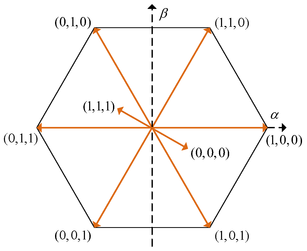
Figure 1 shows the topology of a three-phase two-level inverter. Here, U d c is the DC voltage; L and R are the filter inductance and equivalent parasitic resistance, respectively; e a , e b , e c and i a , i b , i c correspond to the three-phase AC grid voltages and inverter output currents, respectively; S x i ( x = a , b , c ; i = 1 , 2 ) represents the switching states of the power devices. The two switching devices in each phase leg operate in complementary conduction. S x 1 = 1 indicates that the upper switching device is turned ON, while S x 1 = 0 indicates that the upper switching device is turned OFF. The valid combinations of these switching states generate eight distinct discrete space voltage vectors, as listed in Table 1, with their positions in the space vector diagram shown in Figure 2.
Ideally, the inverter in the α β stationary coordinate system can be modeled as follows:
L d i α β d t = u α β R i α β e α β ,
where u α β = [ u α ; u β ] , u α , and u β are the output voltages of the inverter; i α β = [ i α ; i β ] , i α and i β are the output current of the inverter; e α β = [ e α ; e β ] , and e α and e β are the AC voltage.
Assuming that the sampling period is T, the current prediction expression at time t k + 1 can be obtained by discretizing (1) as follows:
i α β ( k + 1 ) = 1 R T L i α β ( k ) + T L u α β ( k ) e α β ( k ) ,
where x ( k ) denotes the value of the variable x at time t k ; x ( k + 1 ) represents the value of variable x at time t k + 1 .
To compensate for the inherent computational delay in the model predictive control strategy, the following compensation mechanism is adopted: First, the optimal voltage vectors u α ( k ) and u β ( k ) obtained in the previous control cycle are substituted into (2), computing the predicted currents i α ( k + 1 ) and i β ( k + 1 ) at time t k + 1 . Subsequently, all candidate voltage vectors u α β ( k + 1 ) shown in Figure 2 are sequentially substituted into (3) to compute their corresponding predicted currents i α β ( k + 2 ) at time t k + 2 . This achieves delay compensation based on two-step prediction, written as follows:
i α β ( k + 2 ) = 1 R T L i α β ( k + 1 ) + T L u α β ( k + 1 ) e α β ( k + 1 ) ,
where x ( k + 2 ) denotes the value of the variable x at t k + 2 .
When the sampling frequency is significantly higher than the system’s fundamental frequency, it is reasonable to assume that the grid voltage vector remains approximately constant over one sampling period, i.e., e α β ( k + 1 ) e α β ( k ) . The compensation of the reference current is achieved using the vector angle compensation method, expressed as follows:
i α β r e f ( k + 2 ) = i α β r e f ( k ) e j 2 π T ,
where i α β r e f ( k ) is the given reference current.
To determine the optimal voltage vector, the cost function defined in (5) evaluates the current tracking performance for each candidate vector. By minimizing the cost function, the optimal voltage vector is selected and applied to the inverter switching actions in the next control cycle.
J = i α β r e f ( k + 2 ) i α β ( k + 2 ) 2 .
As clearly seen from (3), the predicted current is strongly coupled with the inductance parameters L and resistance parameters R. When external factors cause the actual parameters of the device to deviate from the modeled parameters (a phenomenon termed parameter mismatch), significant errors arise. The following section will derive detailed expressions to quantify this error.

2.2. The Effect of Parameter Mismatch

MPC is very sensitive to the change of parameters. The actual filter inductance and parasitic resistance are assumed to be L 0 and R 0 , while L and R are used to represent the filter inductance and parasitic resistance used in the mathematical model. Therefore, the errors of filter inductance and parasitic resistance can be expressed as Δ L = L 0 L and Δ R = R 0 R , respectively, and (2) can be written as follows:
i ¯ α β ( k + 1 ) = 1 R + Δ R L + Δ L T i α β ( k ) + T L + Δ L u α β ( k ) e α β ( k ) ,
where i ¯ α β ( k + 1 ) is the predicted current considering the influence of parameter mismatch.
Taking the error on the α -axis as an example, this paper defines it as ε , which means the difference between (2) and (6).
ε = i α ( k + 1 ) i ¯ α ( k + 1 ) .
Substituting (2) and (6) into (7), we can obtain the following:
ε = T L ( L + Δ L ) ( Δ R L R Δ L ) i α ( k ) Δ L u α ( k ) e α ( k ) .
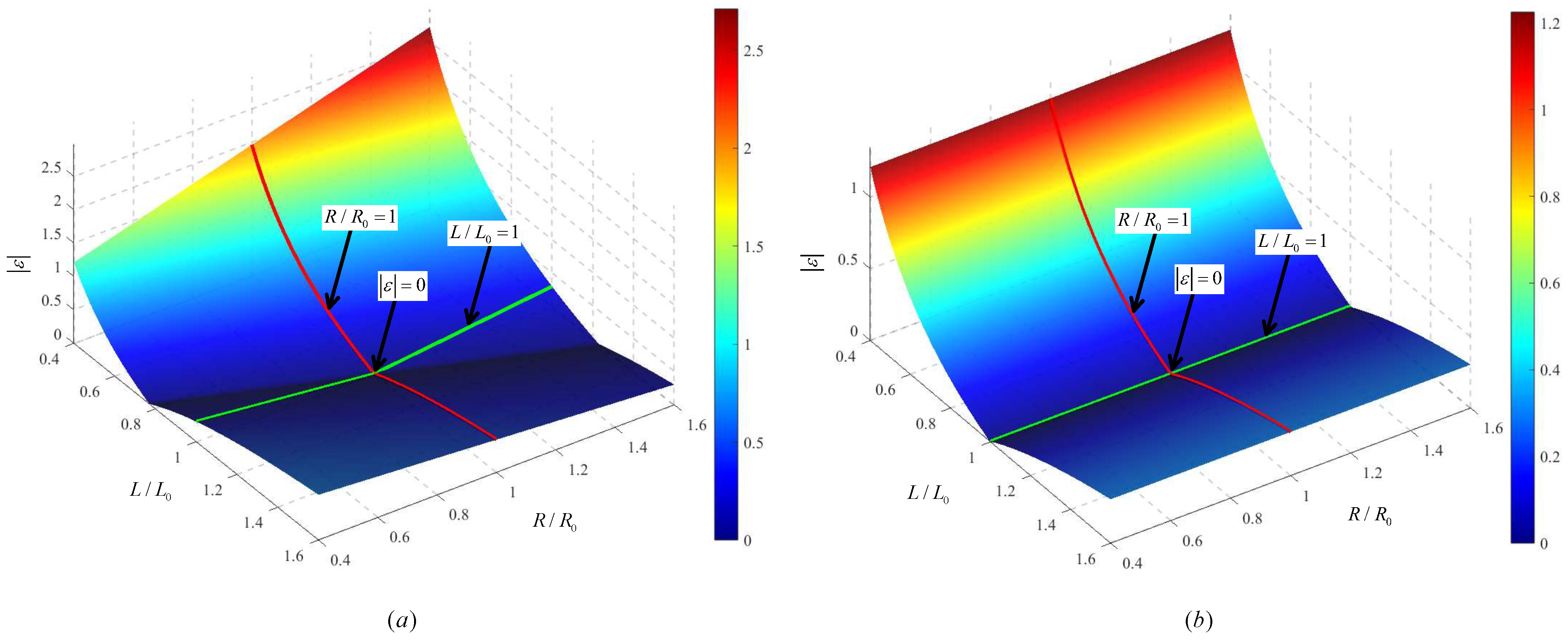
For analyzing the error expression, assume that during the current control cycle, u α = 0 ,   u β = 0 is the optimal vector. Figure 3 shows the absolute prediction error ε under specific parameter combinations: Figure 3a,b demonstrate that when the parasitic resistance is large ( R 0 = 1 Ω ), the resistance parameter mismatch significantly compromises control accuracy. Conversely, when resistance is small ( R 0 = 0.02 Ω ), the negative impact of resistance mismatch on control accuracy is substantially reduced.
Both Figure 3a and Figure 3b reveal that inductance mismatch increases the prediction error ε , exhibiting directional dependency: When the actual inductance is smaller than the modeled value ( L / L 0 < 1 ), ε increases sharply; When the actual inductance is larger ( L / L 0 > 1 ), ε also increases but with a slow trend.

3. Proposed Control Strategy

3.1. Ultra-Local Model

To address the reliance of conventional model predictive control on precise mathematical models and its vulnerability to parameter mismatch, this paper uses the ultra-local model as a solution [13]. This approach completely avoids explicit representation of physical parameters such as inductance and resistance, instead establishing a data-driven nonlinear dynamic relationship that depends solely on system input-output data. This model-free characteristic enables significant advantages in scenarios involving unmodeled dynamics or parametric perturbations.
For a typical first-order dynamic system, its ultra-local model can be expressed in the following form:
x ˙ = σ u ( t ) + F ( t ) ,
where x denotes the system output, u ( t ) is the control input, and σ is a design parameter. The critical term F ( t ) , serving as a lumped representation of unknown dynamics, encompasses in real-time the effects of all unmodeled dynamics, external disturbances, and parameter variations. By estimating the time-varying characteristics of F ( t ) online, this model adaptively compensates for control deviations induced by model mismatch. This mechanism fundamentally eliminates the stringent requirement for parameter accuracy in conventional MPC.
Building on [23], this paper constructs the ultra-local model for a 2L-inverter. While considering practical system parameter deviations, the system equation can be written as:
( L 0 + Δ L ) d i α β d t = u α β ( R 0 + Δ R ) i α β e α β .
According to (9) and (10), the ultra-local model of the 2L-inverter can be further derived, as shown in (11):
d i α β d t = σ u α β + 1 L 0 + Δ L σ u α β 1 L 0 + Δ L e α β + ( R 0 + Δ R ) i α β = σ u α β + F α β ,
where F α β is the lumped disturbance of the system; σ is a non-physical parameter of the 2L-inverter. The prediction model in (2) can be rewritten as follows:
i α β ( k + 1 ) = T F α β ( k ) + σ u α β ( k ) + i α β ( k ) .
Under parameter mismatch, the values of σ and F α β deviate, but F α β encapsulates various errors and disturbances with real-time updating. Consequently, the system maintains robust control performance through F α β despite parameter mismatch. This makes accurate calculation of F α β critically important.
To estimate the lumped disturbance term F α β in real-time without relying on system parameters, existing studies widely adopt algebraic identification techniques (Algebraic-MFPC). Processed via the composite trapezoidal formula [24], F α β is calculated as follows:
F α β = 3 ! T F 3 0 T F ( T F 2 δ ) i α β ( δ ) + σ δ ( T F δ ) u α β ( δ ) d δ ,
where T F = n F T , n F is the number of control cycles. Its value needs to be weighed between computational efficiency and estimation accuracy. Engineering practice shows that the reasonable value range of n F is [8,12]. An excessively large n F leads to a significant increase in computational burden, while an overly small n F reduces the accuracy of disturbance estimation due to insufficient data samples. Traditional algebraic identification requires iterative calculations based on historical data. When the reference command undergoes a step change, a large data window introduces inertial delay, limiting the tracking response speed of F α β . Optimizing n F merely achieves a trade-off between computational complexity and steady-state accuracy without fundamentally improving the response speed during transient processes.

3.2. Adaptive Super-Twisting Sliding Mode Observer

To address the inherent limitations of algebraic methods, a strategy using a sliding mode observer (SMO) to estimate the dynamic component was proposed in [25]. However, this approach introduces chattering into the control system, adversely affecting both dynamic and steady-state performance [26]. The super-twisting sliding mode algorithm (STSMO), a second-order sliding mode technique proposed by Levant [27], effectively suppresses chattering while preserving the strong robustness of conventional SMO. This is achieved by transferring the high-frequency switching discontinuity from the control signal u to its derivative u ˙ .
The STSMO design requires only the sliding surface information and is directly applicable when the relative degree of the system with respect to the sliding variable is 1. However, a key challenge hinders its practical application: difficulty in parameter tuning due to the typically unknown precise boundaries of the dynamic component.
To meet the requirements of model-free predictive current control for the 2L-inverters, this section proposes an improved observer design with the following two key modifications:
(1) Replacing linear error feedback with an exponential adaptive law, where this nonlinear regulation mechanism significantly enhances transient response performance;
(2) Substituting the sign function with a hyperbolic tangent function (tanh) to achieve smooth chattering suppression. Building on these improvements, a three-level cascade-structured adaptive super-twisting sliding mode observer (ASTSMO) is constructed, governed by the following dynamic equations:
d i ^ α β d t = σ u α β + F ^ α β ,
F ^ α β = λ 1 tanh ( k 1 e ) + v ,
d v d t = λ 2 ( t ) tanh ( k 2 e ) ,
where i ^ α β is the observed value of current; e = i α β i ^ α β , denotes current observation error; u α β represents the control input voltage; λ 1 is a fixed gain coefficient, taking a positive real number; k 1 , k 2 is the nonlinear adjustment coefficient, positive real number; and λ 2 ( t ) is a time-varying adaptive gain.
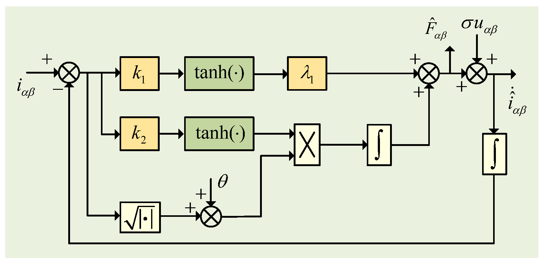
Firstly, the current observation error e is entered into the hyperbolic tangent function processing layer; λ 1 tanh ( k 1 e ) constitutes a proportional channel to generate a fast response component; λ 2 ( t ) tanh ( k 2 e ) d t constitutes an adaptive integral channel to generate a disturbance tracking component; the estimated value of the disturbance is output after the two channels are superimposed.
The sign function inherently introduces high-frequency switching, leading to chattering in the estimated disturbance F ^ α β and consequently in the control output, degrading both dynamic and steady-state performance, and potentially exciting unmodeled high-frequency dynamics. The smooth, bounded nature of the tanh function effectively suppresses this chattering phenomenon by providing a continuous approximation of the switching action. This results in smoother control signals, lower output current distortion, and reduced stress on the inverter switches.
The time-varying adaptive gain λ 2 ( t ) is designed as follows:
λ 2 ( t ) = γ | e | 0.5 + θ ,
where γ is the adaptive adjustment coefficient ( γ > 0); θ is the basic gain term ( θ > 0). This adaptation mechanism dynamically adjusts the observer gain based on the magnitude of the observation error | e | . When | e | is large (e.g., during transients or large disturbances), λ 2 ( t ) increases significantly, providing stronger corrective action to accelerate convergence. Conversely, when | e | is small (near steady-state), λ 2 ( t ) reduces towards θ , mitigating the risk of excessive control effort and high-frequency oscillations (chattering) that are common drawbacks of fixed high-gain SMOs. This adaptive property enhances the overall transient response speed while improving steady-state smoothness and robustness.
After the observer converges, the lumped disturbance estimate is as follows:
F ^ α β = λ 1 tanh ( k 1 e ) λ 2 ( t ) tanh ( k 2 e ) d t ,
The structure diagram of the adaptive super-twisting sliding mode observer designed according to (14a–c)–(16) is shown in Figure 4.

3.3. Stability Proof

Proposition 1.
For the adaptive super-twisting sliding mode observer defined by (14a–c), the observer error e converges to zero in finite time when the following conditions hold:
a. The lumped disturbance F α β is bounded, i.e., there exists a constant F max > 0 such that | F α β ( t ) | F max for all t;
b. The gain parameters satisfy λ 2 > F max , γ > 0 , λ 1 > 0 ;
c. The nonlinear regulation coefficients k 1 , k 2 are sufficiently large.
Proof. 
The finite-time convergence proof proceeds through five key stages:
(1) Error Dynamics: establish the differential equation governing the observer error e.
(2) Lyapunov Function: construct a composite Lyapunov function candidate V = V 1 + V 2 .
(3) Derivative and Substitution: compute d V / d t and substitute the error dynamics and adaptive gain law.
(4) Inequality Scaling: bound dV/dt using strategic inequalities to isolate negative definite terms.
(5) Finite-Time Conclusion: show d V / d t κ V 1 2 , invoking the finite-time stability theorem. □
From the ultra-local model (9) and observer Equation (14a), the observer error dynamics yields the following:
d e d t = d i α β d t d i ^ α β d t = F α β F ^ α β .
Substituting (14b) in the following:
d e d t = F α β + λ 1 tanh ( k 1 e ) v .
The Lyapunov function is constructed as (19), V is a positive definite function.
V = V 1 + V 2 = 1 2 e 2 + 1 2 γ λ 2 λ 2 * 2 ,
where λ 2 is the lower bound of the ideal gain, satisfying λ 2 * > F max + η ( η > 0 ) .
d V d t = d V 1 d t + d V 2 d t = e d e d t + 1 γ λ 2 λ 2 * d λ 2 d t ,
Substituting (18) into (20) results in the following:
d V 1 d t = e F α β + λ 1 tanh ( k 1 e ) v ,
The adaptive gain derivation of (15) is written as follows:
d λ 2 d t = γ 2 | e | 0.5 d e d t sign ( e ) ,
Since | e | 0.5 is singular at e = 0 , a regularization factor needs to be introduced. Let ρ = | e | 1 / 2 + ξ , ξ be small constants greater than 0.
d λ 2 d t = γ 2 ρ 1 d e d t sign ( e ) ,
Substituting (18), (21) and (23) into (20) results in the following:
d V d t = e F α β + λ 1 tanh ( k 1 e ) v + 1 γ λ 2 λ 2 * ρ 1 sign ( e ) d e d t = e F α β + e λ 1 tanh ( k 1 e ) e v + 1 2 λ 2 λ 2 * ρ 1 sign ( e ) d e d t = e F α β + e λ 1 tanh ( k 1 e ) e v + 1 2 λ 2 λ 2 * ρ 1 sign ( e ) F + λ 1 tanh ( k 1 e ) v .
The following proves that it converges in finite time, using three inequalities to scale:
e λ 1 tanh ( k 1 e ) λ 1 k 1 e 2 cosh 2 ( 0 ) = λ 1 k 1 e 2 ,
e v 1 2 e 2 + 1 2 v 2 ,
1 2 ( λ 2 λ 2 * ) ρ 1 sign ( e ) F α β 1 2 | λ 2 λ 2 * | ρ 1 sign ( e ) F max 1 2 ( λ 2 λ 2 * ) 2 ρ 2 + 1 2 F max 2 ,
The conditions for the establishment of (25a) are: when | x | is close to 0, tanh ( x ) sech 2 ( 0 ) . The validity of (25b) can be proven by using Young’s inequality. Under parameter condition | F α β | F max , λ 2 * > F max + η , (25c) can be proven to hold. Combining (25a)–(25c) and selecting sufficiently large λ 1 and k 1 , we obtain the following:
d V d t λ 1 k 1 1 2 e 2 + 1 2 v 2 1 2 η ρ 1 + 1 2 F max 2 ,
By (14c), we know that v is bounded and take the following:
λ 1 k 1 > 1 2 + 1 2 v max 2 + F max 2 , η > F max 2 ,
Then there exists κ > 0 such that the following is met:
d V d t κ V 1 2 ,
According to the finite-time stability theorem, the observer error e converges to zero in finite time T 2 V ( 0 ) 1 / 2 κ .

3.4. ASTSMO-MFPC Strategy

Substitute F ^ α β with the dynamically estimated term F α β obtained from the stabilized ASTSMO into (12), and consider delay compensation, written as follows:
i α β ( k + 2 ) = T F ^ α β ( k ) + σ u α β ( k + 1 ) + i α β ( k + 1 ) ,
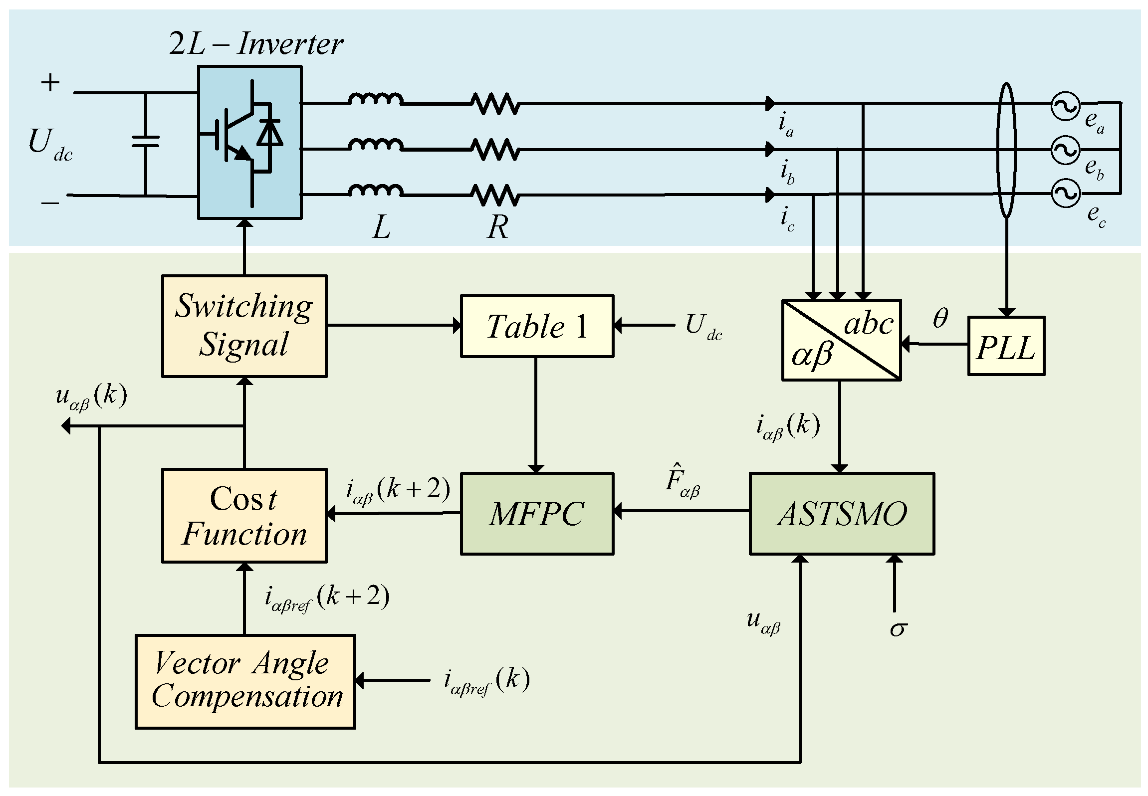
The cost function defined in (5) is still employed for receding-horizon optimization. In summary, the block diagram of the proposed adaptive super-twisting sliding mode observer-based model-free predictive control for inverter is shown in Figure 5.
The execution flow of this control algorithm comprises three main steps: First, the adaptive super-twisting sliding mode observer estimates the dynamic component of the inverter’s ultra-local model in real-time; Second, the obtained estimate is substituted into the prediction model equation to compute the predicted state at the next sampling instant, followed by a global optimization calculation based on the predefined cost function; Finally, the optimal voltage vector that minimizes the cost function value is selected to generate corresponding switching signals. This control strategy requires no precise physical parameters of the inverter system, thus exhibiting remarkable robustness.

4. Simulation Verification

To verify the effectiveness of the proposed algorithm, a simulation model was established and compared with both conventional model predictive current control (MPC) and algebraic-based model-free predictive current control (Algebraic-MFPC). Identical circuit parameters were used for all methods, operating at low voltage levels. Relevant simulation parameters are listed in Table 2.

4.1. Steady-State Results Under Parameter Matching

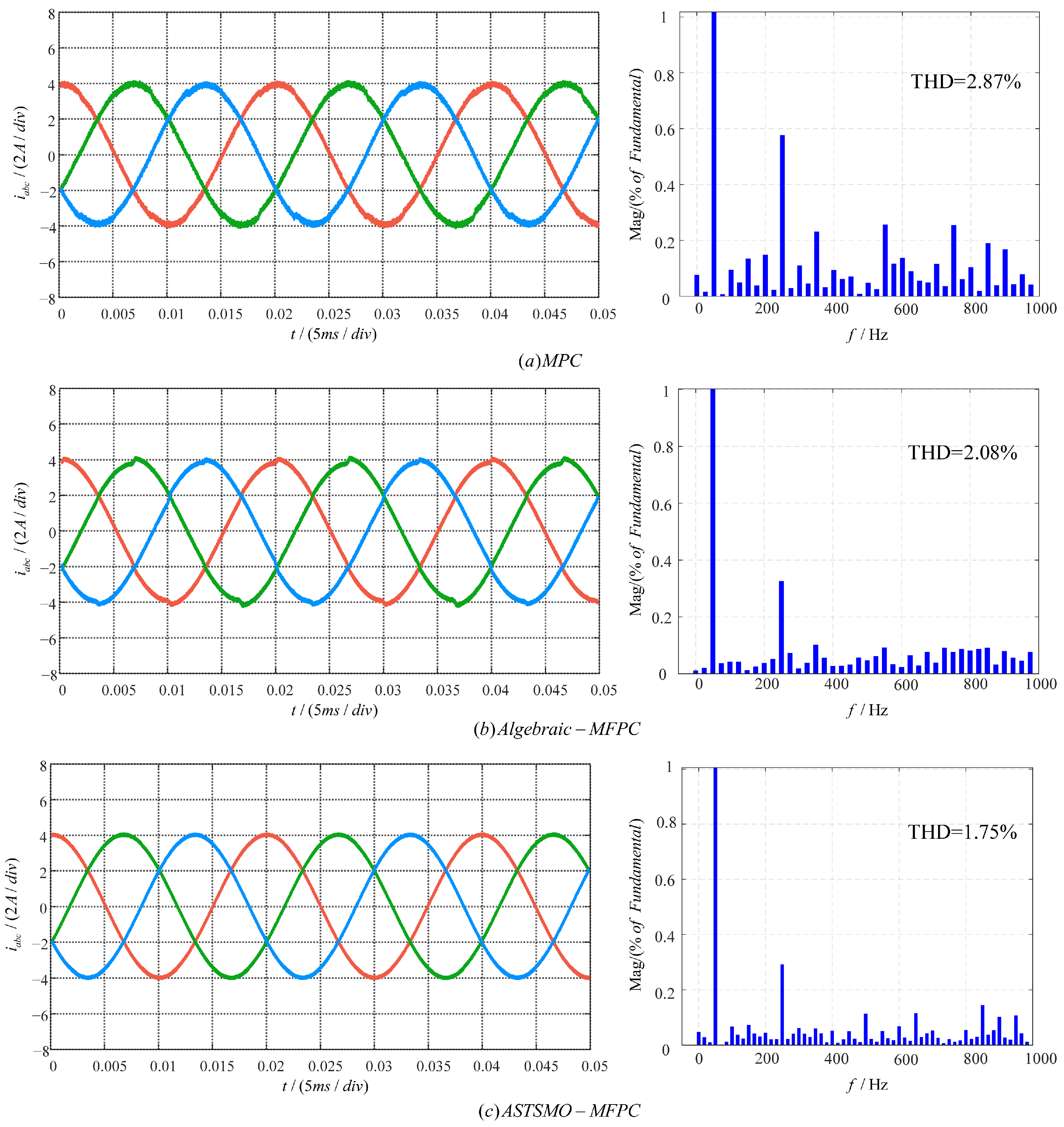
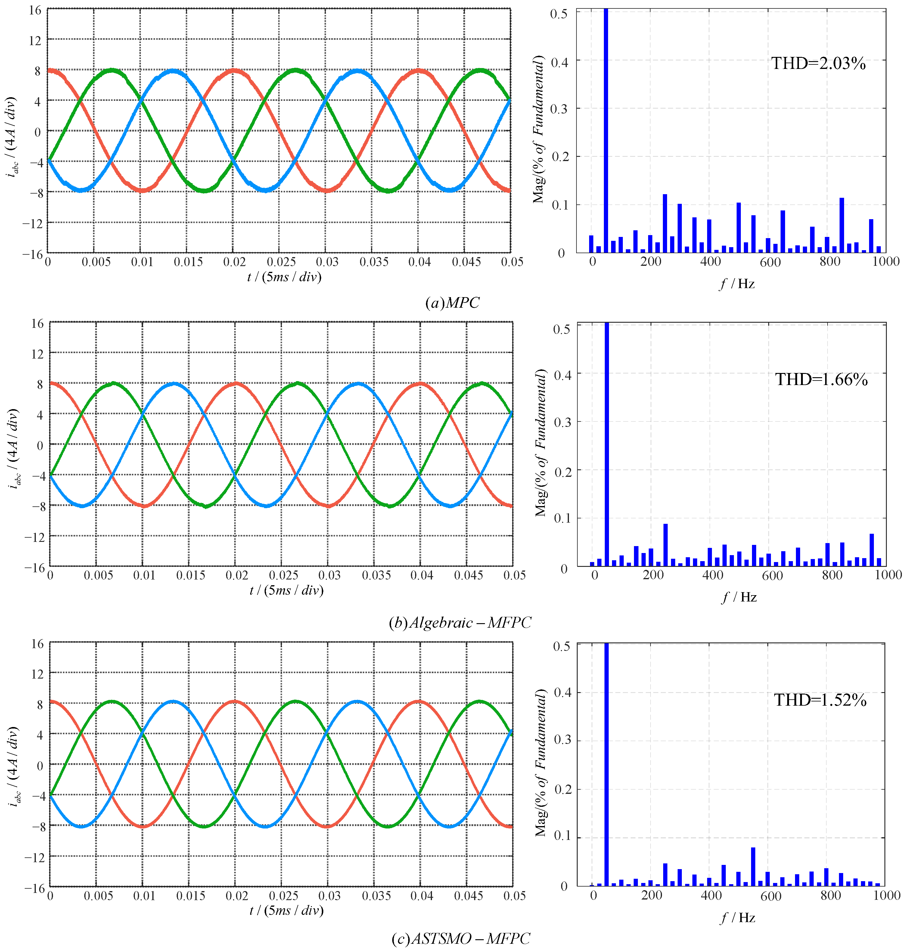
To validate effectiveness, the steady-state performance of the ASTSMO-MFPC was compared via simulations with MPC and Algebraic-MFPC. Figure 6 and Figure 7 present the output current waveforms and corresponding total harmonic distortion (THD) analyses for the three methods under parameter matching at reference currents with peak values equal to 4 A and 8 A, respectively. THD values under varying reference currents are summarized in Table 3.
Simulation results demonstrate that under parameter-matched conditions, all three strategies achieve steady-state reference current tracking while maintaining THD within industry-accepted standards. Detailed analysis reveals: (1) With accurate parameter matching, MPC delivers acceptable performance meeting basic requirements; (2) Both MFPC methods outperform conventional MPC, as clearly evidenced by Table 3 data showing significantly lower THD values for MFPC strategy at identical reference currents; (3) Figure 6 and Figure 7 indicate that Algebraic-MFPC exhibits slight overshoot at phase peaks, whereas the proposed ASTSMO-MFPC maintains superior current amplitude accuracy with smoother waveforms; (4) Table 3 THD data conclusively proves ASTSMO-MFPC achieves the lowest THD across all tested currents (4–12 A), substantially outperforming both MPC and Algebraic-MFPC. For example, at 8 A, its THD ( 1.52 % ) is lower than MPC’s 2.03 % and Algebraic-MFPC’s 1.66 % , with this advantage persisting as current increases.
In summary, under parameter-matched conditions, the proposed ASTSMO-MFPC demonstrates optimal performance in both current amplitude accuracy and harmonic suppression (THD reduction).

4.2. Results Under Parameter Mismatching

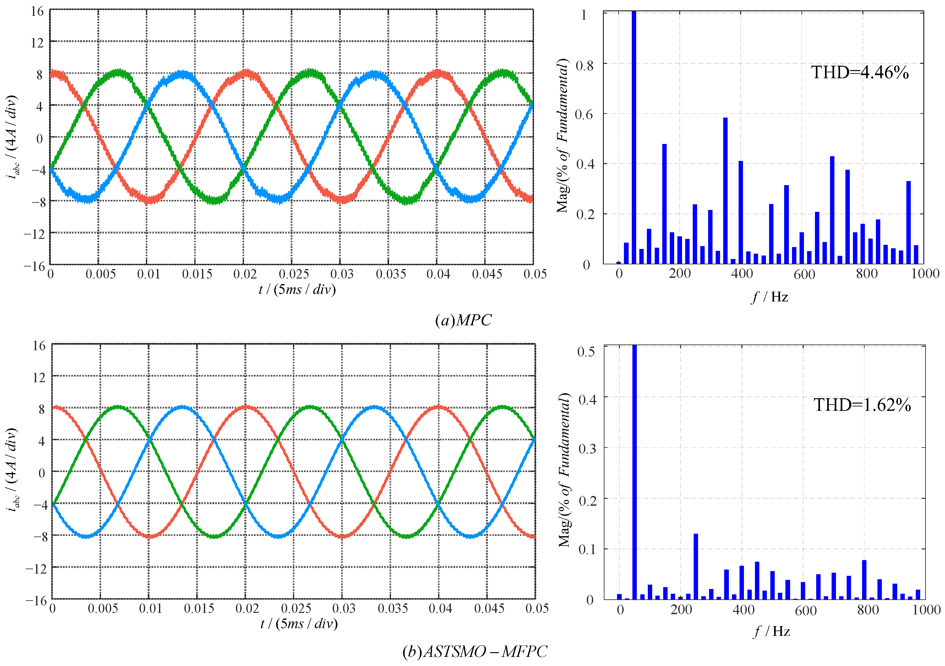
To validate the parameter robustness of the proposed method, this paper conducts a comparative study between ASTSMO-MFPC and MPC under model parameter mismatch conditions. The simulation sets the reference current to 8 A and configures the inductance parameter in the control algorithm to L / L 0 = 0.5 .
Figure 8 displays the output current waveforms of both methods under parameter mismatch. Visually, the MPC output exhibits significant distortion with degraded waveform smoothness and a doubled THD value. In contrast, ASTSMO-MFPC maintains accurate tracking of the reference sinusoidal wave without observable distortion, showing minimal THD variation.
Table 4 presents the THD values of both strategies under parameter mismatch conditions at reference currents ranging from 6 A to 12 A. At each operating point, the MPC strategy exhibits significantly increased THD, while the ASTSMO-MFPC maintains near-constant performance. These results demonstrate that while conventional MPC suffers severe performance degradation under parameter mismatch, the ASTSMO-MFPC method substantially enhances parameter robustness through its observer’s real-time updating of unknown dynamics.

4.3. Dynamic Response

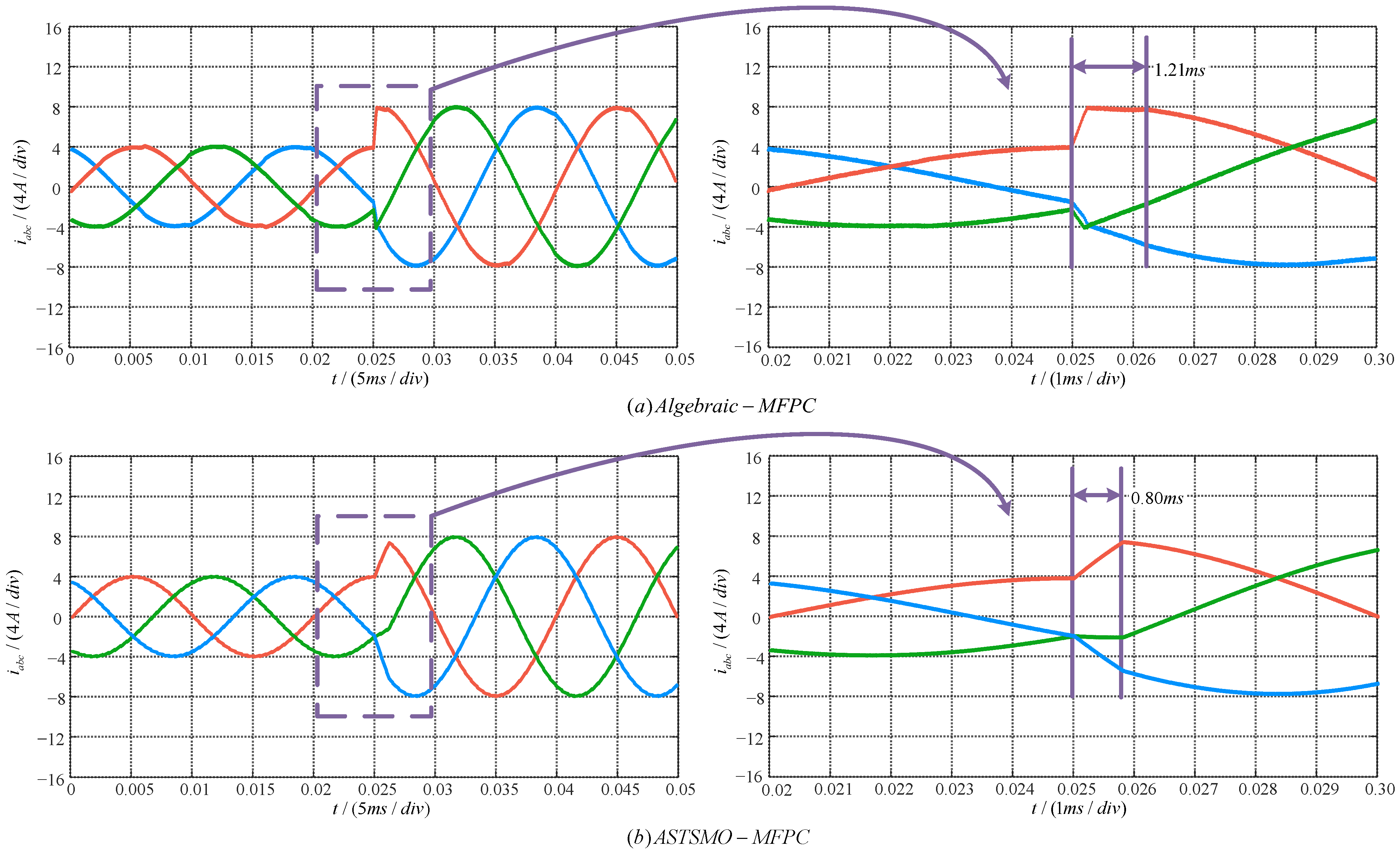
To thoroughly compare the dynamic performance of the proposed ASTSMO-MFPC with Algebraic-MFPC, dynamic tests under reference current step changes were conducted. The test configured the reference current to step-increase from 4 A to 8 A. When the reference current experienced a step change, the response time of Algebraic-MFPC was 1.21 ms. In contrast, ASTSMO-MFPC exhibited a faster dynamic response with its response time significantly reduced to 0.80 ms. This indicates a 34.7 % improvement in system response speed compared to the conventional algebraic method, demonstrating substantial dynamic performance advantages.
This accelerated response is primarily attributed to the core design of the ASTSMO observer, specifically its adaptive gain mechanism. Unlike the algebraic-MFPC which relies on a large window of historical data (introducing inherent inertial delay), the ASTSMO performs real-time estimation. Crucially, during the large observation error transient caused by the step change, the adaptive gain λ 2 ( t ) automatically increases. This higher gain provides a stronger corrective action, enabling the observer to converge much faster onto the rapidly changing true value of the lumped disturbance F α β within the ultra-local model. This rapid and accurate real-time estimation of F α β allows the predictive controller to compute the optimal voltage vector based on the most current system state, fundamentally enabling the faster overall current tracking response observed in Figure 9. The use of the tanh function further ensures this fast convergence occurs smoothly without introducing detrimental chattering. Therefore, the superior dynamic performance stems directly from the ASTSMO’s ability to rapidly adapt and accurately estimate disturbances in real-time, overcoming the latency inherent in the algebraic approach.
To objectively evaluate the computational complexity of the proposed strategy, execution times were measured on an PC with AMD Ryzen5 5600 @ 4.4 GHz processor, providing an assessment of the relative computational burden between conventional MPC and the ASTSMO-MFPC strategy. Key findings are summarized as follows:
In the control actuation stage, both the proposed ASTSMO-MFPC and conventional MPC require traversing all 8 voltage vectors and iteratively evaluating the cost function. The computational complexity of this stage is equal. The additional computational overhead primarily originates from the online ASTSMO estimation module, which dynamically updates the coefficients of the ultra-local model. Consequently, the overall computational complexity of the proposed strategy exhibits only a 21% increase compared to conventional MPC.
This modest increase in complexity poses no barrier to real-time implementation. As conventional MPC is routinely executed at 20–50 kHz on commercial off-the-shelf DSPs and FPGAs, the proposed strategy, with its marginally higher demand, remains firmly within the capabilities of existing hardware platforms.

5. Conclusions

To address the performance degradation of model predictive control caused by parameter mismatch in three-phase inverter systems, this paper proposes a model-free predictive current control strategy based on an adaptive super-twisting sliding mode observer. This strategy integrates model-free concepts into the predictive framework, replacing traditional physical models with a first-order ultra-local model to fundamentally eliminate reliance on precise parameters. By designing an ASTSMO with adaptive gains to accurately estimate unknown dynamic terms in the ULM in real-time, it significantly enhances disturbance rejection capability. Simultaneously, the adaptive gain mechanism simplifies parameter tuning. Simulation results demonstrate that the proposed ASTSMO-MFPC method outperforms conventional MPC and algebraic MFPC in both steady-state harmonic suppression and dynamic response speed. It exhibits stronger parameter robustness and superior comprehensive dynamic–steady-state performance, providing an effective solution for high-performance inverter control under parametric uncertainty.
It is important to note that the simulations presented in this work assume an ideal, balanced sinusoidal grid voltage. The robustness and performance of the proposed ASTSMO-MFPC strategy under practical grid disturbances, such as voltage imbalances, sags, swells, and harmonic distortion, have not been evaluated and represent an essential area for future investigation. Future work will primarily focus on the experimental validation of the ASTSMO-MFPC strategy through embedded implementation (e.g., on DSP or FPGA). This experimental platform will then facilitate a comprehensive comparative study benchmarking the proposed strategy against other advanced model-free predictive control strategies (e.g., predict-then-filter methods) and modern online parameter-identification-based MPC approaches, under a wider range of operating conditions, including grid disturbances and non-linear loads, to further elucidate its relative advantages and application boundaries.

Author Contributions

Conceptualization, W.L., L.G.F., and Z.S.; methodology, W.L.; validation, W.L., Z.S., and R.Z.; formal analysis, W.L.; investigation, W.L.; data curation, Z.S. and R.Z.; writing—original draft preparation, W.L., Z.S., and R.Z.; writing—review and editing, W.L., J.I.L., and A.M.A.; supervision, L.G.F. All authors have read and agreed to the published version of the manuscript.

Funding

This work is supported in part by the National Natural Science Foundation of China, under grant 62003114; the Provincial Natural Science Foundation of Heilongjiang, under grant LH2023F019; the China Postdoctoral Science Foundation, under grant 2020M681097; the Heilongjiang Postdoctoral Fund, under grant LBH-Z20134; the Fundamental Research Funds for the Central Universities, under grant HIT.NSFJG202207; the National Key Laboratory of Laser Spatial Information Foundation, under grant LSI2025WDZC07; Ministerio de Ciencia e Innovación under the project TED2021-130613B-I00 and PID2023-152292OB-I00; “UE—Ministerio de Hacienda y Función Publica—Fondos Europeos—Junta de Andalucía—Consejería de Universidad, Investigación e Innovación project 2024-31824—1828102303”; and ANID/FONDAP/1523A0006 SERC Chile.

Data Availability Statement

The original contributions presented in this study are included in the article. Further inquiries can be directed to the corresponding author.

Conflicts of Interest

The authors declare no conflicts of interest.

References

  1. Luo, W.; Stynski, S.; Chub, A.; Franquelo, L.G.; Malinowski, M.; Vinnikov, D. Utility-Scale Energy Storage Systems: A Comprehensive Review of Their Applications, Challenges, and Future Directions. IEEE Ind. Electron. Mag. 2021, 15, 17–27. [Google Scholar] [CrossRef]
  2. Sui, Z.; Sun, Q.; Wang, R.; Li, D.; Wang, P. The Grid-Connected Inverter Stability Enhancement Control Based on Impedance Instability Region Elimination. IEEE Trans. Power Electron. 2025, 40, 9606–9624. [Google Scholar] [CrossRef]
  3. Alharbi, Y.; Darwish, A.; Ma, X. A Review of Model Predictive Control for Grid-Connected PV Applications. Electronics 2025, 14, 667. [Google Scholar] [CrossRef]
  4. Zafra, E.; Granado, J.; Lecuyer, V.B.; Vazquez, S.; Alcaide, A.M.; Leon, J.I.; Franquelo, L.G. Computationally Efficient Sphere Decoding Algorithm Based on Artificial Neural Networks for Long-Horizon FCS-MPC. IEEE Trans. Ind. Electron. 2024, 71, 39–48. [Google Scholar] [CrossRef]
  5. Shin, E.C.; Chae, H.G.; Roh, C. Advancing Discontinuous-Model Predictive Control for High Performance Inverters via Optimized Zero-Voltage State Selection Based on Offset Voltage. Appl. Sci. 2025, 15, 5532. [Google Scholar] [CrossRef]
  6. Liu, T.; Wang, X. Unified Voltage Control for Grid-Forming Inverters. IEEE Trans. Ind. Electron. 2024, 71, 2578–2589. [Google Scholar] [CrossRef]
  7. Guazzelli, P.R.U.; Pereira, W.C.; Oliveira, C.M.R.; Castro, A.G.; Aguiar, M.L. Weighting Factors Optimization of Predictive Torque Control of Induction Motor by Multiobjective Genetic Algorithm. IEEE Trans. Power Electron. 2018, 34, 6628–6638. [Google Scholar] [CrossRef]
  8. Shi, X.; Zhu, J.; Li, L.; Lu, D.D.C. Model-Predictive-Based Duty Cycle Control with Simplified Calculation and Mutual Influence Elimination for AC/DC Converter. IEEE J. Emerg. Sel. Top. Power Electron. 2019, 7, 504–514. [Google Scholar] [CrossRef]
  9. Shen, X.; Liu, J.; Liu, G.; Zhang, J.; Leon, J.I.; Wu, L.; Franquelo, L.G. Finite-Time Sliding Mode Control for NPC Converters with Enhanced Disturbance Compensation. IEEE Trans. Circuits Syst. I: Regul. Pap. 2025, 72, 1822–1831. [Google Scholar] [CrossRef]
  10. Chen, Z.; Qiu, J.; Jin, M. Adaptive Finite-Control-Set Model Predictive Current Control for IPMSM Drives with Inductance Variation. IET Electr. Power Appl. 2017, 11, 874–884. [Google Scholar] [CrossRef]
  11. Lin, C.K.; Yu, J.; Lai, Y.S.; Yu, H.C. Improved Model-Free Predictive Current Control for Synchronous Reluctance Motor Drives. IEEE Trans. Ind. Electron. 2016, 63, 3942–3953. [Google Scholar] [CrossRef]
  12. Guo, F.; Yang, T.; Diab, A.M.; Yeoh, S.S.; Bozhko, S.; Wheeler, P. An Enhanced Virtual Space Vector Modulation Scheme of Three-Level NPC Converters for More-Electric-Aircraft Applications. IEEE Trans. Ind. Appl. 2021, 57, 5239–5251. [Google Scholar] [CrossRef]
  13. Michel, F.; Cédric, J. Model-Free Control. Int. J. Control 2013, 86, 2228–2252. [Google Scholar]
  14. Guo, L.; Jin, N.; Gan, C.; Luo, K. Hybrid Voltage Vector Preselection-Based Model Predictive Control for Two-Level Voltage Source Inverters to Reduce the Common-Mode Voltage. IEEE Trans. Ind. Electron. 2019, 67, 4680–4691. [Google Scholar] [CrossRef]
  15. Li, H.; Li, X.; Chen, Z.; Mao, J.; Huang, J. Model-Free Adaptive Integral Backstepping Control for PMSM Drive Systems. J. Power Electron. 2019, 19, 1193–1202. [Google Scholar]
  16. Zhang, Y.; Jiang, T.; Jiao, J. Model-Free Predictive Current Control of a DFIG Using an Ultra-Local Model for Grid Synchronization and Power Regulation. IEEE Trans. Energy Convers. 2020, 35, 2269–2280. [Google Scholar] [CrossRef]
  17. Liu, J.; Shen, X.; Alcaide, A.M.; Yin, Y.; Leon, J.I.; Vazquez, S.; Wu, L.; Franquelo, L.G. Sliding Mode Control of Grid-Connected Neutral-Point-Clamped Converters Via High-Gain Observer. IEEE Trans. Ind. Electron. 2022, 69, 4010–4021. [Google Scholar] [CrossRef]
  18. Wang, Y.; Li, H.; Liu, R.; Yang, L.; Wang, X. Modulated Model-Free Predictive Control with Minimum Switching Losses for PMSM Drive System. IEEE Access 2020, 8, 20942–20953. [Google Scholar] [CrossRef]
  19. Cao, Y.L.; Cao, J.A.; Song, X.; Liu, Y.J. Research on Vector Control of PMSM Based on an Improved Sliding Mode Observer. Power Syst. Prot. Control 2021, 49, 104–111. [Google Scholar]
  20. Bagheri, F.; Bonaldo, J.; Guler, N.; Rivera, M.; Wheeler, P.; Lima, R. Enhanced Sliding Mode Control for Dual MPPT Systems Integrated with Three-Level T-Type PV Inverters. Energies 2025, 18, 3344. [Google Scholar] [CrossRef]
  21. Do, T.A.; Pham, Q.H.; Giap, V.N.; Nguyen, Q.D.; Vu, P. Homogeneous disturbance observer based on sliding mode observer and controller for T-type inverter. J. Electr. Eng. Technol. 2024, 19, 1671–1683. [Google Scholar] [CrossRef]
  22. Luo, W.; Vazquez, S.; Liu, J.; Gordillo, F.; Franquelo, L.G.; Wu, L. Control System Design of a Three-Phase Active Front End Using a Sliding-Mode Observer. IEEE Trans. Syst. Man, Cybern. Syst. 2020, 52, 739–748. [Google Scholar] [CrossRef]
  23. Ma, C.; Li, H.; Yao, X.; Zhang, Z.; Belie, F.D. An Improved Model-Free Predictive Current Control with Advanced Current Gradient Updating Mechanism. IEEE Trans. Ind. Electron. 2020, 68, 11968–11979. [Google Scholar] [CrossRef]
  24. Li, F.; Zheng, T.; He, N.; Cao, Q. Data-Driven Hybrid Neural Fuzzy Network and ARX Modeling Approach to Practical Industrial Process Identification. IEEE/CAA J. Autom. Sin. 2022, 9, 1702–1705. [Google Scholar] [CrossRef]
  25. Jin, N.; Chen, M.; Guo, L.; Li, Y.; Chen, Y. Double-Vector Model-Free Predictive Control Method for Voltage Source Inverter with Visualization Analysis. IEEE Trans. Ind. Electron. 2021, 69, 10066–10078. [Google Scholar] [CrossRef]
  26. Wang, D.; Liu, X. Sensorless control of PMSM with improved adaptive super-twisting sliding mode observer and IST-QSG. IEEE Trans. Transp. Electrif. 2024, 11, 721–731. [Google Scholar] [CrossRef]
  27. Chalanga, A.; Kamal, S.; Fridman, L.M.; Bandyopadhyay, B.; Moreno, J.A. Implementation of Super-Twisting Control: Super-Twisting and Higher Order Sliding-Mode Observer-Based Approaches. IEEE Trans. Ind. Electron. 2016, 63, 3677–3685. [Google Scholar] [CrossRef]
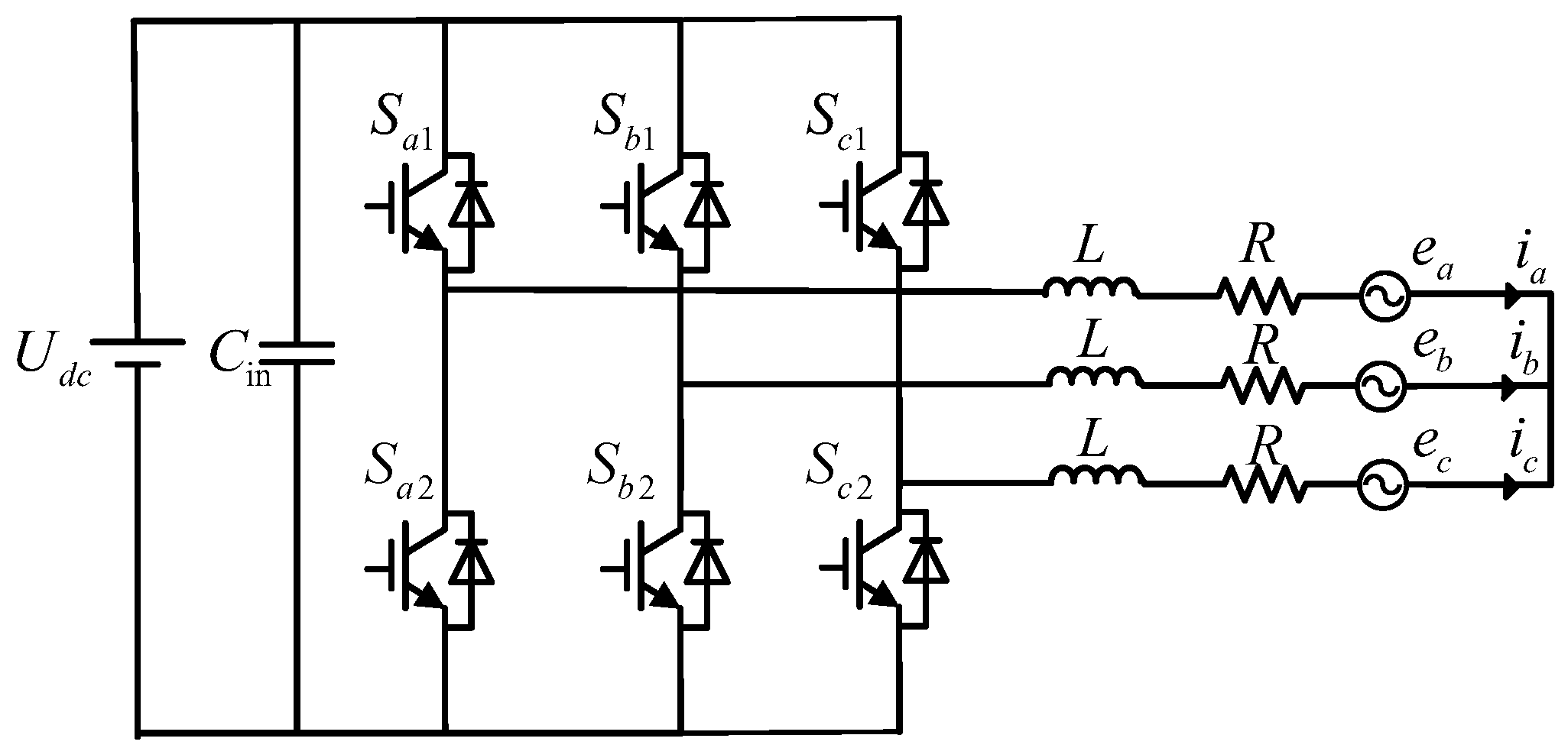
Figure 1. Two-level three-phase inverter.
Energies 18 04570 g001
Figure 2. Discrete voltage vector.
Energies 18 04570 g002
Figure 3. Diagram of ε : (a) when L 0 = 0.005 H , R 0 = 1 Ω ; (b) when L 0 = 0.005 H , R 0 = 0.02 Ω .
Energies 18 04570 g003
Figure 4. Diagram of ASTSMO structure.
Energies 18 04570 g004
Figure 5. Diagram of system control structure.
Energies 18 04570 g005
Figure 6. The simulation results when the reference current is 4A: (a) MPC strategy; (b) Algebreic-MFPC strategy; (c) ASTSMO-MFPC strategy.
Energies 18 04570 g006
Figure 7. The simulation results when the reference current is 8A: (a) MPC strategy; (b) Algebreic-MFPC strategy; (c) ASTSMO-MFPC strategy.
Energies 18 04570 g007
Figure 8. Output current results under parameter mismatch: (a) MPC strategy; (b) ASTSMO-MFPC strategy.
Energies 18 04570 g008
Figure 9. Diagram of reference current step: (a) Algebreic-MFPC strategy; (b) ASTSMO-MFPC strategy.
Energies 18 04570 g009
Table 1. Switching states and voltage vector.
Switching States
( S a 1 , S b 1 , S c 1 )
U α U β
(0,0,0)00
(0,0,1) U d c / 3 U d c / 3
(0,1,0) U d c / 3 U d c / 3
(0,1,1)−2 U d c / 3 0
(1,0,0)2 U d c / 3 0
(1,0,1) U d c / 3 U d c / 3
(1,1,0) U d c / 3 U d c / 3
(1,1,1)00
Table 2. Simulation parameters.
ParameterValue
DC voltage U d c ( V ) 120
Effective value of AC line voltage e ( V ) 60
Filter inductor L ( H ) 0.005
Parasitic resistance R ( Ω ) 0.05
Sampling frequency f ( k H z ) 20
Scale factor σ 500
Basic gain θ 25
Proportional gain λ 1 150
Nonlinear coefficient k 1 80
Nonlinear coefficient k 2 120
Adaptive coefficient γ 16
Table 3. THD under different reference with parameter matching.
ReferenceTHD of MPCTHD of Algebraic-MFPCTHD of ASTSMO-MFPC
4 A2.87%2.08%1.75%
6 A2.35%1.79%1.67%
8 A2.03%1.66%1.52%
10 A1.90%1.54%1.37%
12 A1.80%1.44%1.30%
Table 4. THD under different reference with parameter mismatching.
ReferenceTHD of MPCTHD of ASTSMO-MFPC
4 A5.88%1.80%
6 A5.06%1.72%
8 A4.46%1.62%
10 A3.98%1.42%
12 A3.85%1.33%
Disclaimer/Publisher’s Note: The statements, opinions and data contained in all publications are solely those of the individual author(s) and contributor(s) and not of MDPI and/or the editor(s). MDPI and/or the editor(s) disclaim responsibility for any injury to people or property resulting from any ideas, methods, instructions or products referred to in the content.