A Transformer-Based Hybrid Neural Network Integrating Multiresolution Turbulence Intensity and Independent Modeling of Multiple Meteorological Features for Wind Speed Forecasting

Abstract

Aiming at the nonlinear, nonstationary, and multiscale fluctuation characteristics of wind speed series, this study proposes a wind speed-forecasting framework that integrates multi-resolution turbulence intensity features and a Transformer-based hybrid neural network. Firstly, based on multi-resolution turbulence intensity and stationary wavelet transform (SWT), the original wind speed series is decomposed into eight pairs of mean wind speeds and turbulence intensities at different time scales, which are then modeled and predicted in parallel using eight independent LSTM sub-models. Unlike traditional methods treating meteorological variables such as air pressure, temperature, and wind direction as static input features, WaveNet, LSTM, and TCN neural networks are innovatively adopted here to independently model and forecast these meteorological series, thoroughly capturing their dynamic influences on wind speed. Finally, a Transformer-based self-attention mechanism dynamically integrates multiple outputs from the four sub-models to generate final wind speed predictions. Experimental results averaged over three datasets demonstrate superior accuracy and robustness, with MAE, RMSE, MAPE, and $R^2$ values around 0.65, 0.87, 23.24%, and 0.92, respectively, for a 6 h forecast horizon. Moreover, the proposed framework consistently outperforms all baselines across four categories of comparative experiments, showing strong potential for practical applications in wind power dispatching.

1. Introduction

As the proportion of wind energy, a green and renewable energy source, continues to increase in the global energy structure, how to improve the operational efficiency, stability, and dispatching capability of wind farms has become an important topic in current renewable energy system research. Wind speed forecasting, as a fundamental part of wind power system operation and grid-connected control, plays a crucial role in power system dispatching optimization and operation management. Due to the highly nonlinear, non-stationary, and uncertain characteristics of wind speed, the task of wind speed forecasting has long faced great challenges in terms of modeling accuracy, generalization ability, and real-time performance.

Physical modeling methods are among the earliest approaches used for wind speed forecasting. These methods mainly rely on numerical weather-prediction models, such as the weather research and forecasting (WRF) model and the mesoscale model 5 (MM5) model [1], and construct medium- or long-term wind speed-forecasting frameworks on a global or regional scale by systematically modeling the dynamic processes of the wind field, thermodynamic processes, terrain features, and boundary layer disturbances. Although physical modeling methods have good physical consistency and interpretability, they suffer from problems such as complex modeling, high computational cost, sensitivity to boundary conditions, and difficulty in frequent updates, making them unsuitable for short-term or ultra-short-term forecasting tasks [2,3].

Statistical models take wind speed time series as the modeling object and construct formal statistical relationship models based on historical data to perform regression or extrapolation on data trend changes. This type of method was widely applied in short-term wind speed forecasting in the early stage. Common models include autoregressive moving average model (ARMA) [4], autoregressive integrated moving average model (ARIMA) [5], markov autoregressive models [6], and support vector regression (SVR) [7,8,9]. However, these models generally rely on assumptions of stationarity and linearity, making it difficult to handle complex nonlinear wind speed signals, which leads to significant limitations in generalization ability and long-term forecasting accuracy.

In recent years, data-driven intelligent modeling methods have gradually replaced traditional physical modeling and statistical regression models, becoming a research hotspot. Deep learning, with its strong nonlinear modeling and adaptive capabilities, has been widely applied in the field of wind speed forecasting. Among them, structures such as deep neural network (DNN), convolutional neural network (CNN), long short-term memory (LSTM), and gated recurrent unit (GRU) have been widely used to model the temporal dynamic process of wind speed. Noorollahi et al. [10] used artificial neural network (ANN) to forecast wind speed in both temporal and spatial dimensions. Ak et al. [11] trained multilayer perceptron neural networks using a multi-objective genetic algorithm to realize wind speed interval forecasting, and combined the extreme learning machine with the nearest neighbor method for short-term wind speed prediction. Kadhem et al. [12] developed a wind speed data-forecasting method based on the Weibull distribution and ANN, which can utilize the essential dependence between wind speed and seasonal weather variations to model wind speed data based on seasonal wind changes within a specific time range. Wang et al. [13] proposed a hybrid deep learning method based on wavelet transform, deep belief network, and quantile regression for deterministic and probabilistic wind speed forecasting. Hu et al. [14] used deep learning to extract wind speed patterns from data-rich wind farms and fine-tuned the model with data from newly built wind farms, realizing a knowledge transfer-based wind speed-forecasting method that effectively reduces prediction error. Khodayar et al. [15] introduced a rough deep neural network—built on stacked autoencoders and denoising autoencoders—for ultra-short- and short-term wind speed forecasting. By adding rough neural networks to boost robustness, it achieved lower RMSE and MAE than both conventional deep and shallow models.

However, although these models have made some progress in prediction accuracy, they still suffer from problems such as being prone to local optima, overfitting, slow convergence speed, and weak generalization ability [16]. Moreover, the inherent non-stationarity and strong disturbance characteristics of wind speed data cause single models to lack prediction stability in the face of severe fluctuations or sudden changes, and their generalization ability is limited. In response, researchers have gradually introduced data-preprocessing strategies, such as denoising the original wind speed series to reduce sequence randomness, or decomposing the wind speed series into multiple sub-series of different frequencies, and then forecasting the preprocessed wind speed data. Liu et al. [17] proposed a novel multi-step wind speed-forecasting model combining variational mode decomposition (VMD), singular spectrum analysis (SSA), LSTM and extreme learning machine (ELM). Comparative experiments with eight other models showed that this model performed best and was more robust in multi-step forecasting performance and trend information extraction. Liu et al. [18] proposed a wind speed-forecasting model based on wavelet packet decomposition (WPD), CNN, and CNN-LSTM. Comparative experiments with eight models demonstrated its robustness and superior performance, especially in wind speed mutation cases. Ref. [19] established a hybrid framework for multi-step wind speed forecasting based on WPD, complete ensemble empirical mode decomposition with adaptive noise (CEEMDAN) and ANN, and compared the advantages and disadvantages of different decomposition methods. Santhosh et al. [20] applied ensemble empirical mode decomposition (EEMD) to the original data and used wavelet neural network for forecasting. Zhang et al. [21] used optimized variational mode decomposition (OVMD) to eliminate redundant noise. Peng et al. [22] first used wavelet transform (WT) to decompose wind speed data into more stationary components in the wind speed-decomposition process. Peng et al. [23] used the wavelet soft threshold denoising (WSTD) method to filter out redundant information in the original wind speed data during the decomposition process. Xu et al. [24] proposed a wind speed-forecasting method based on seasonal and trend decomposition using Loess (STL), which decomposes wind speed series into seasonal, trend, and residual components and applies models such as attention-based long LSTM and ARIMA-LSTM to significantly improve forecasting accuracy and responsiveness to extremes.

The above methods have verified the positive role of data-preprocessing techniques in wind speed forecasting. However, due to the fact that the level of wind speed uncertainty cannot be accurately quantified through time-frequency analysis and mode decomposition, the bias in multi-step forecasting remains large. At present, signal-processing methods for original wind speed series cannot effectively handle medium- and long-term forecasts beyond 4 h. According to the power spectrum of the atmospheric boundary layer, actual wind speed can be divided into two components [25]: the first part is the mean wind speed, and the second component is the turbulent wind speed. Numerous studies have shown that turbulent wind speed has a significant impact on wind power output. Kim et al. [26] found that the wake effect significantly increased turbulence intensity and wind shear, and that the high turbulence intensity and wind shear gradient in the second stage led to an increase in fatigue load, with the damage equivalent load being 30–50% higher than that of the first stage. Siddiqui et al. [27] conducted a complete 3D numerical transient simulation for offshore vertical axis wind turbines under varying turbulence intensity levels of incoming wind. The results showed that when turbulence intensity increased from $5\%$ to $25\%$, the performance of the wind turbine dropped by approximately $23\%$ to $42\%$ compared with the non-turbulence case. Due to the above effects, turbulent wind speed should be considered in wind speed forecasting.

In addition, to further enhance the performance of wind speed forecasting, scholars have devoted efforts to integrating multiple models to achieve complementary advantages of various methods, thereby more comprehensively leveraging the predictive power of hybrid models and providing stronger support for wind speed forecasting. Neshat et al. [28] integrated VMD with an improved arithmetic optimization algorithm (IAOA) to process wind speed data and established a hybrid model combining quantum convolutional neural network (QCNN) and bidirectional long short-term memory (BiLSTM) for wind speed prediction. Meanwhile, a fast and efficient hyper-parameters tuner (HPT) was introduced to adjust the parameters and architecture of the hybrid model. Experimental results showed that its accuracy and stability significantly outperformed five existing machine learning models and two hybrid models. Memarzadeh et al. [29] decomposed the original wind speed data using wavelet transform and utilized the crow search algorithm to determine the hyperparameters of LSTM. The results indicated that this hybrid model outperformed the single LSTM model.

Alternatively, some researchers have attempted to incorporate intelligent optimization algorithms to automatically tune the hyperparameters of prediction models, aiming to further improve model performance and forecasting accuracy. These methods perform optimization in the search space, thereby avoiding the limitations of manual parameter setting, and have demonstrated promising potential in wind speed-prediction tasks. Samadianfard et al. [30] applied the whale optimization algorithm (WOA) to a multilayer perceptron (MLP) model, and the results showed that this model outperformed multilayer perceptron-genetic algorithm (MLP-GA) and traditional MLP at all stations, achieving better performance in evaluation metrics such as RMSE. Wang et al. [31], based on regression plot (RP) and SVR, introduced the cuckoo optimization algorithm (COA) to optimize model parameters and constructed a COA-SVR wind speed-forecasting model, which demonstrated stable and superior performance in multi-step forecasting and practical applications in wind farms. Wang et al. [32] proposed a CNN-LSTM ensemble optimized by a multi-objective chameleon swarm algorithm (CSA), achieving notable improvements in ultra-short-term wind speed forecasting.

However, most ensemble systems allocate weights to the outputs of sub-models through optimization algorithms or multi-objective optimization algorithms and perform linear summation to obtain the final prediction result. Since wind speed has high instability and volatility, simple linear summation is not conducive to the organic integration of sub-model predictions, limiting the performance of the ensemble system. The Transformer architecture, due to its global attention mechanism advantage in sequence modeling, shows great potential in wind speed forecasting. Bommodi et al. [33] combined Improved complete ensemble empirical mode decomposition (ICEEMDAN) with Transformer to model the multi-scale fluctuation structure of wind speed. Zha et al. [34] introduced convolutional mechanisms into the Transformer encoder module to enhance the model’s ability to extract local dynamic features. These studies indicate that the Transformer-based dynamic fusion mechanism has better modeling efficiency and generalization ability compared to traditional weighted ensemble strategies, and is especially suitable for non-stationary time series with high noise and high-frequency disturbances like wind speed. Besides the evolution of modeling architectures, input feature construction is also a key factor affecting wind speed forecasting performance.

Current research has gradually expanded from modeling a single wind speed sequence to collaborative modeling of multiple meteorological factors. Variables such as temperature, air pressure, and wind direction are widely used to enhance the model’s predictive perception capability. Zhu et al. [35] proposed a modeling method that integrates environmental features, background features, and multi-scale spatial information, significantly improving ultra-short-term wind speed-forecasting performance. Yu et al. [36] combined multi-feature fusion strategies with frequency-domain feature-extraction techniques to achieve joint deterministic and probabilistic wind speed forecasting, demonstrating stronger modeling robustness and generalization ability. However, existing studies mostly treat these meteorological variables as static external features, directly concatenating them as model inputs, ignoring their own temporal dynamic characteristics and potential coupled evolutionary relationships with wind speed.

Based on the above literature review and the strengths and limitations of existing models, this study proposes a novel integrated system to maximize the predictive potential of wind speed and other relevant meteorological data, aiming to improve short- and medium-term wind speed-forecasting performance. First, stationary wavelet transform (SWT) with the Sym8 wavelet basis is employed in conjunction with turbulence intensity computation to perform multi-scale decomposition of the original wind speed data, yielding eight sequences representing mean wind speed and turbulent wind speed at different temporal scales. Second, the eight groups of decomposed wind speed and turbulence intensity features are fed into eight independently constructed LSTM sub-models to obtain initial predictions. Third, three meteorological factors—air pressure, temperature, and wind direction—are incorporated and modeled using WaveNet, LSTM, and temporal convolutional network (TCN) architectures respectively, thereby supplementing the external environmental information relevant to wind speed forecasting. Finally, the eight sub-component wind speed predictions and four meteorological prediction outputs are integrated into a Transformer model. Leveraging the self-attention mechanism, the model captures deep temporal dependencies among multiple variables, enabling nonlinear feature fusion and final wind speed output.

The proposed method is validated from the following perspectives: (1) Comparison with six classical single neural network prediction models; (2) Comparison with two neural network models based on data-preprocessing techniques; (3) Comparison with a model where the nonlinear combination output module in the proposed model is replaced by a linear combination output based on optimization algorithms (such as CSA, WOA); (4) Comparison with a model that uses only the LSTM model based on turbulence intensity and SWT, without incorporating multiple meteorological features and multiple time scales.

The main contributions of this study are as follows:

(1)

Systematic introduction of multi-scale turbulence intensity as a measure of wind speed uncertainty. Through SWT decomposition, joint modeling of mean wind speed and turbulence intensity features is achieved, significantly enhancing the model’s capability to capture rapid fluctuations in wind speed.

(2)

For the first time in wind speed forecasting, independent prediction sub-models were constructed for other meteorological features to extract their evolutionary trend characteristics, and the results were unified with the primary wind speed model within a Transformer architecture. This differs from previous approaches that treated other meteorological factors as static inputs. Additionally, considering the cyclical nature of wind direction, the cosine and sine values of wind direction were innovatively employed as both the input and output of the TCN.

(3)

Utilization of the self-attention mechanism within the Transformer to enable dynamic, nonlinear fusion of sub-model outputs, effectively addressing the limitations of fixed-weight combinations under imbalanced data conditions and achieving more adaptive prediction integration.

(4)

Demonstration of strong multi-step forecasting extensibility and structural flexibility, with excellent adaptability to abrupt wind fluctuations and long-term forecasting scenarios, indicating promising engineering applicability and deployment potential.

The remainder of this paper is organized as follows: Section 2 presents the materials and methods used in the ensemble forecasting system. Section 3 provides data description, evaluation metrics and details about the framework of the proposed ensemble system. Section 4 introduces four experiments and the corresponding analyses. Further Conclusions and future work are provided in Section 5.

2. Materials and Methods

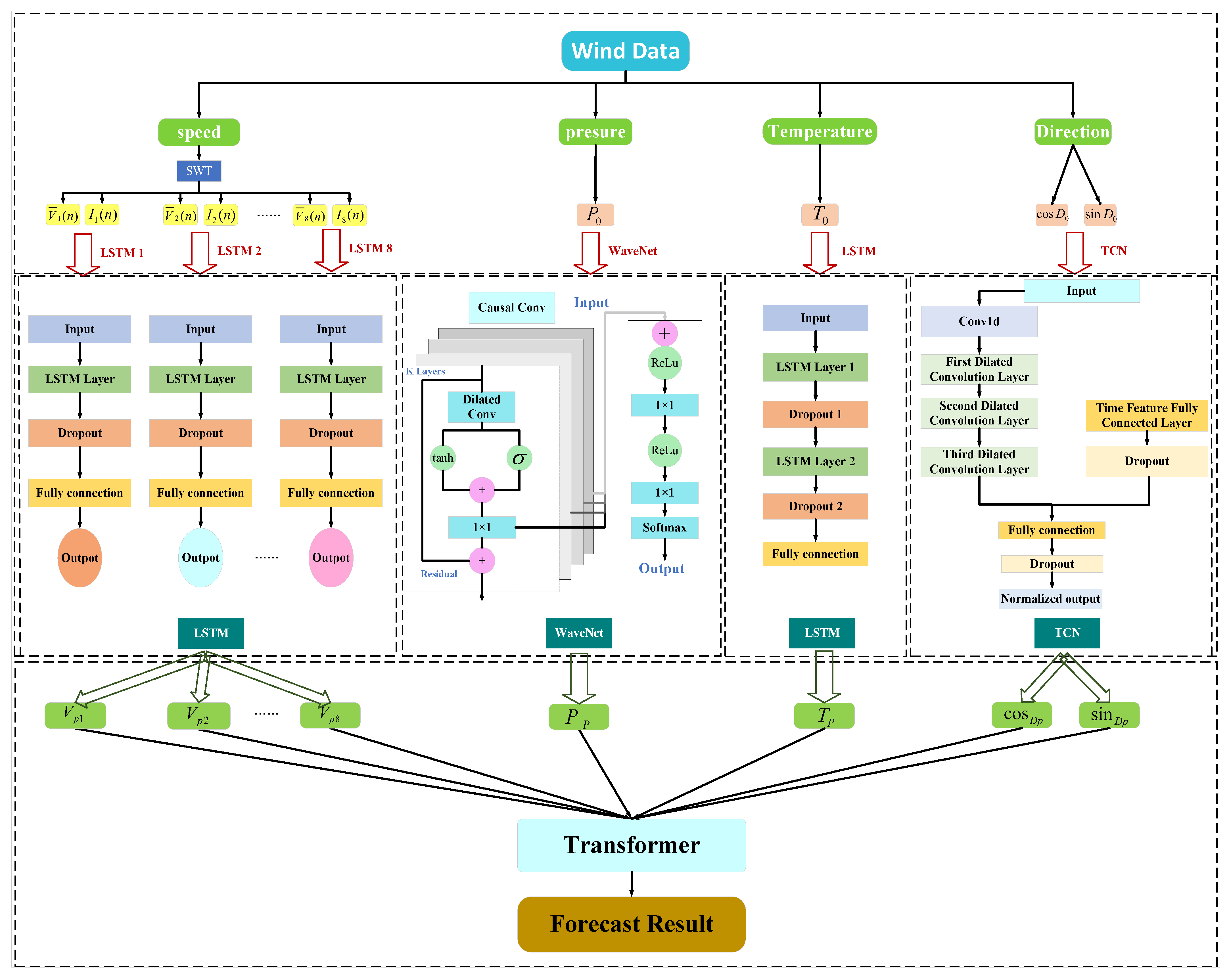
As shown in Figure 1, the proposed wind speed-prediction system consists of three modules: wind speed-decomposition module, multi-feature prediction module, and combination module. The details of the prediction system are described as follows:

2.1. Wind Speed Decomposition Module

The original wind speed series can be decomposed into a mean wind speed component that reflects the trend and a turbulent wind speed component that represents uncertainty. This study introduces turbulence intensity as a metric for wind speed uncertainty and employs SWT to extract real-time multi-resolution wind speed and turbulence intensity, constructing a feature set for prediction.

Wind speed uncertainty is an inherent characteristic present across different time scales. According to the theory presented in Reference [25], the wind speed spectrum at 65 m, as shown in Figure 2, exhibits three distinct peaks: The first peak corresponds to weather systems with a 100 h timescale, reflecting frontal and synoptic influences; the second peak represents diurnal variations at a 24 h timescale; while the third peak indicates turbulence with timescales ranging from 10 min to 10 h.

According to spectral theory, actual wind speed is the superposition of mean wind speed and turbulent wind speed. Traditional Reynolds-averaging methods decompose flow-field variables into mean and turbulent components but only provide statistical turbulence intensity over a period rather than real-time turbulence intensity at a specific resolution.

To address this, our study extends the Reynolds-averaging method via SWT, performing multi-level decomposition to obtain mean wind speed and turbulent wind speed at different time scales, along with their corresponding feature spaces.

Let the original wind speed time series be denoted as $v_n=\{v_1,v_2,\dots ,v_T\}$, where the low-frequency and high-frequency subseries at the m-th level are recursively computed through SWT:

$$L{v}_m\left(n\right)=\sum _{i}L{v}_{m-1}\left(i\right)h(2i-1),$$

(1)

$$H{v}_m\left(n\right)=\sum _{i}L{v}_{m-1}\left(i\right)g(2i-1),$$

(2)

given initial conditions:

$$L{v}_0\left(n\right)=H{v}_0\left(n\right)=v\left(n\right),$$

(3)

where $h(2n-i)$ denotes scaling function that is more compact at lower frequencies, and $g(2n-i)$ denotes wavelet function that concentrates on higher frequencies.

The temporal resolution of wind speed subseries is determined by the original sampling rate of 10 min; thus, the time resolution at the m-th level equals 10 × minutes. The low-frequency subseries represents the mean wind speed trend at the corresponding resolution, it also represents the mean wind speed on a pried of $10\times 2^m$ min, which is given as:

$${\overline{v}}_m\left(n\right|T)=L{v}_m\left(n\right|T),T=10\times 2^m$$

(4)

Once the mean wind speed is obtained, the turbulent wind speed $\delta v\left(n\right)$ is expressed as:

$$\delta v\left(n\right)=v\left(n\right)-\overline{v}\left(n\right)$$

(5)

According to the Reynolds-averaged method, the turbulence standard deviation is:

$$\sigma \left(n\right)=\sqrt{{\displaystyle \frac{1}{T}}\sum _{i=1}^T{\left[\delta v\left(n\right)\right]}^2}$$

(6)

Whereas the turbulence standard deviation is also a statistic calculated on a consecutive sequence of turbulent wind speed $\delta v\left(n\right)$, the DWT can also be used to obtain the real-time turbulence standard deviation at multiple resolutions as well:

$$L{\sigma }_0^2\left(n\right)={\left[\delta v\left(n\right)\right]}^2$$

(7)

Additionally, at the m-th level of decomposition one has

$$L{\sigma }_m^2(n\mid T)=\sum _{i}L{\sigma }_{m-1}^2(i\mid T)h(2n-i),T=10\times 2^m$$

(8)

$${\sigma }_m(n\mid T)=\sqrt{L{\sigma }_m^2(n\mid T)},T=10\times 2^m$$

(9)

Finally, the turbulence intensity at scale T is defined by

$$I(n\mid T)={\displaystyle \frac{{\sigma }_m(n\mid T)}{{\overline{v}}_m(n\mid T)}}.$$

(10)

It is noteworthy that when applying the SWT for multi-level decomposition of wind speed, the low-frequency components require scaling and energy rebalancing. Since SWT is a redundant transform with translation invariance, each decomposition level generates approximation and detail coefficients of the same length as the original signal, causing the total energy to inflate as the decomposition level increases. Through empirical scaling and global energy rebalancing, the actual amplitude of the low-frequency components can be restored, ensuring consistency with the long-term variations of actual wind speeds. This provides a reliable foundation for subsequent turbulence intensity calculation and wind speed forecasting analysis.

2.2. Multi-Feature Prediction Module

2.2.1. Air Pressure Prediction Module

To achieve precise modeling and prediction of atmospheric pressure, this study incorporates the WaveNet model. Originally proposed by DeepMind [37], WaveNet is a temporal sequence generation model based on deep CNN. Its primary advantage lies in combining causal convolutions with dilated convolutions to effectively capture long-term dependencies while maintaining strict temporal consistency during prediction.

In the WaveNet framework, let the input atmospheric pressure time series be denoted as $x=\{x_1,x_2,\dots ,x_T\}$.The model extracts deep temporal features through stacked dilated causal convolutional layers. To preserve causality, when predicting the value at time t, the model utilizes only information from time t and earlier. Dilated convolutions expand the receptive field by inserting fixed intervals between convolutional kernel elements, enabling the model to capture broader historical context with fewer layers, thereby effectively modeling long-range dependencies.

In the computational implementation, the output of the l-th convolutional layer is governed by a gating mechanism, expressed as:

$$z^{\left(l\right)}=\sigma \left(W_f^{\left(l\right)}{\ast }_{d_l}{z}^{(l-1)}\right)·tanh\left(W_g^{\left(l\right)}{\ast }_{d_l}{z}^{(l-1)}\right)$$

(11)

where $z^{\left(0\right)}=x$, ${\ast }_{d_l}$ denotes the dilated convolution at dilation rate $d_l$, $W_f^{\left(l\right)}$ and $W_g^{\left(l\right)}$ are the filter weights for feature transformation and gating activation respectively, $\sigma (·)$ is the sigmoid activation function, and $tanh(·)$ is the hyperbolic tangent. The Hadamard product “·” implements nonlinear transformation and control of the signal.

To further enhance the model’s representational capacity and training efficiency, WaveNet incorporates residual connections. This mechanism ensures each layer’s output is derived not only through convolutional transformations but also via direct summation with the input, formulated as:

$$r^{\left(l\right)}=z^{\left(l\right)}+r^{(l-1)}$$

(12)

This architecture enables the model to effectively prevent gradient vanishing while increasing network depth, ensuring stable performance in long-sequence modeling. Ultimately, the outputs from all residual blocks are aggregated and transformed through a series of $1\times 1$ convolutional layers to produce the predicted atmospheric pressure value ${\widehat{y}}_t$ at each corresponding timestep.

2.2.2. Temperature Prediction Module

To model and forecast temperature time series, this study employs LSTM networks. Originally proposed by Hochreiter in 1997 [38], LSTM represents a specialized recurrent neural network architecture designed to address the gradient vanishing and explosion problems inherent in conventional RNNs when processing long sequences. As shown in Figure 3, unlike standard RNNs, LSTM incorporates gating mechanisms within its neural units, enabling selective retention and forgetting of information. This architecture provides enhanced capability for modeling long-term temporal dependencies.

2.2.3. Wind Direction Prediction Module

To effectively capture the dynamic patterns within wind direction time series, this study employs the Temporal Convolutional Network as the primary prediction model. TCN is a convolution-based sequence modeling approach that offers several advantages over traditional recurrent neural networks, including parallel computation, large receptive fields, and stable gradient propagation, making it particularly well-suited for modeling long-term dependencies in sequential data.

The core structure of the TCN consists of multiple stacked one-dimensional convolutional layers, integrating two key mechanisms: causal convolution and dilated convolution. Causal convolution ensures that the output at any given time depends only on the current and previous inputs, thus preserving the temporal causality of the sequence. Dilated convolution allows the receptive field to expand exponentially without increasing the number of parameters, enabling the model to capture long-range temporal dependencies efficiently. In addition, TCN introduces residual connections to enhance training stability in deep networks, effectively mitigating the vanishing gradient problem and accelerating model convergence.

Given the periodic nature of wind direction data, the angular values are transformed into two-dimensional vectors using their sine and cosine components before modeling. This transformation preserves the continuity of circular data and avoids artificial discontinuities between 0° and 360°. The converted features are then input into the TCN, which outputs predictions in the same sine and cosine form, ensuring consistency between input and output as well as preserving physical interpretability.

2.2.4. Nonlinear Combination Output Module

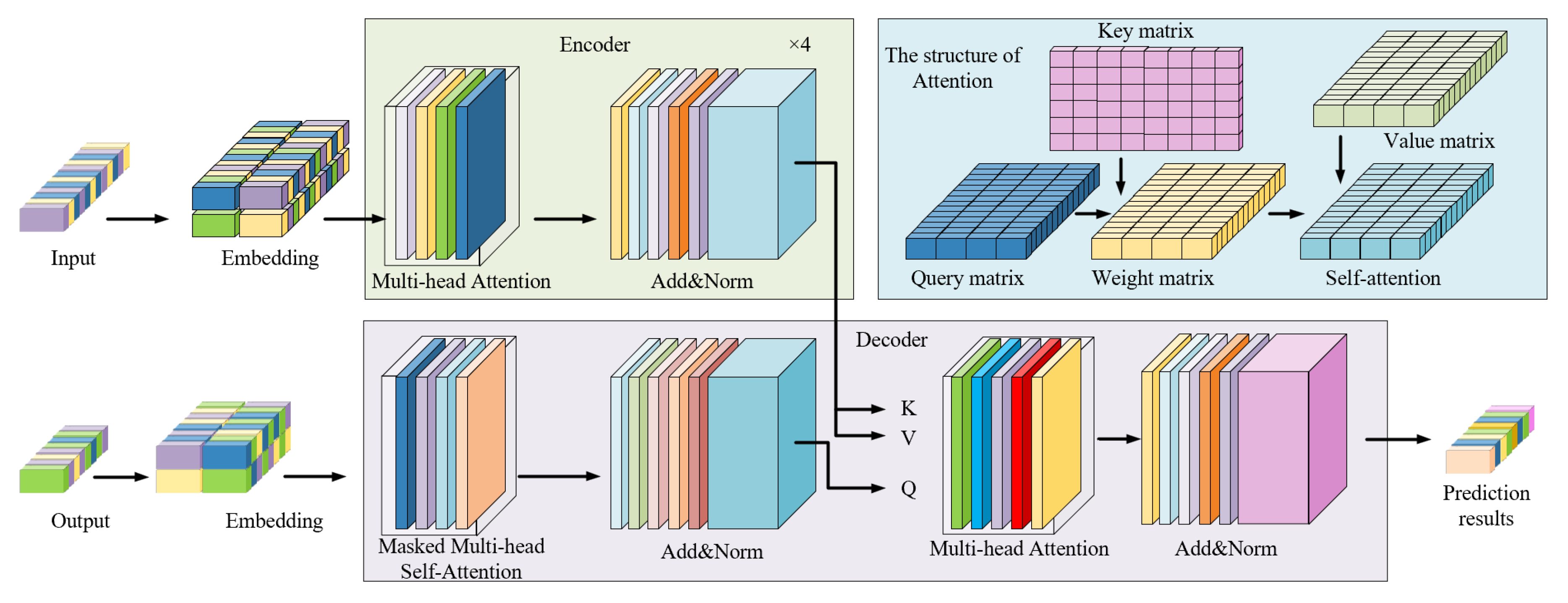
Transformer is a deep neural network architecture based on the self-attention mechanism, originally proposed by Vaswani et al. [39]. Due to its outstanding performance in capturing global dependencies within sequential data, it has been widely applied in time series-forecasting tasks in recent years. Unlike traditional recurrent neural networks, the Transformer eliminates the need for recurrence and instead relies entirely on attention mechanisms for sequence modeling, offering advantages such as high parallelization efficiency and strong capability in modeling long-range dependencies.

At the core of the Transformer lies the multi-head self-attention mechanism, which enables the model to adaptively capture contextual relationships across different positions in the sequence at each time step. By projecting each position in the input sequence into queries, keys, and values, the model can effectively learn the dependencies among different time steps. The use of multiple attention heads further enhances the model’s ability to extract features from various subspaces.

As shown in Figure 4, the Transformer is typically composed of multiple stacked encoder and decoder layers. Each layer integrates a multi-head self-attention module and a position-wise feed-forward network, along with residual connections and layer normalization to ensure training stability and improved representational capacity.

3. The Proposed Ensemble System

3.1. Data Description

This study employed three wind speed datasets collected from sites located at different latitudes and longitudes, providing geographical diversity and covering regions with distinct climatic conditions. Dataset 1 was publicly released by Li et al. (2019) on Mendeley Data [40], which was originally introduced in their research article [41]. It was collected in Jilin Province, China, spanning January–December 2013 with a 10 min sampling frequency. In this study, the target variable was wind speed at 65 m, accompanied by corresponding meteorological features, namely air pressure, air temperature, and 65-m wind direction. Dataset 2 and Dataset 3 were obtained from the Wind Resource Database hosted by the National Renewable Energy Laboratory (NREL) (https://wrdb.nrel.gov/data-viewer, accessed on 24 August 2025), corresponding to sites in California (36.16° N, 118.24° W, year 2013) and Florida (28.21° N, 82.50° W, year 2016), respectively. For both datasets, wind speed at 100 m was used as the target, with air temperature, pressure, and wind direction as input features, sampled every 10 min. These three datasets, originating from Northeast China, the western United States, and the southeastern United States, provide diverse climatic and geographical contexts, which enhance the evaluation of model generalization capability. The statistical characteristics of the three datasets are summarized in

Table 1. Descriptive statistics of meteorological variables (with units) across three datasets.

Dataset	Variable	Count	Mean	Std	Min	Median	Max	Skewness	Kurtosis
Dataset 1	Wind Speed (m/s)	52,557	6.215	3.125	0.2	5.725	22.7	0.878	1.131
	Air Temperature (°C)	52,557	4.514	15.308	−32.04	5.494	32.09	−0.253	−1.03
	Air Pressure (hPa)	52,557	896.674	7.527	855	897	916	−0.168	−0.121
	Wind Direction (°)	52,557	214.836	94.838	0.01	217.7	360	−0.693	−0.204
Dataset 2	Wind Speed (m/s)	52,560	5.82	3.851	0.02	5.06	24.56	1.21	1.561
	Air Temperature (°C)	52,560	14.074	8.402	−9.69	14.07	33.67	−0.201	−0.59
	Air Pressure (hPa)	52,560	826.47	4.788	807.6	827	838.2	−0.522	0.424
	Wind Direction (°)	52,560	214.825	99.586	0.01	236.65	360	−0.463	−0.893
Dataset 3	Wind Speed (m/s)	52,560	6.03	2.606	0.02	5.97	21.12	0.232	−0.045
	Air Temperature (°C)	52,560	24.297	3.673	4.47	24.47	33.33	−0.964	1.508
	Air Pressure (hPa)	52,560	1004.729	3.288	987.4	1004.8	1015.2	−0.34	1.255
	Wind Direction (°)	52,560	139.898	90.58	0	113.92	360	1.004	0.085

The table reports descriptive statistics including count, mean, standard deviation (Std), minimum (Min), median, maximum (Max), skewness, and kurtosis for each meteorological variable.

.

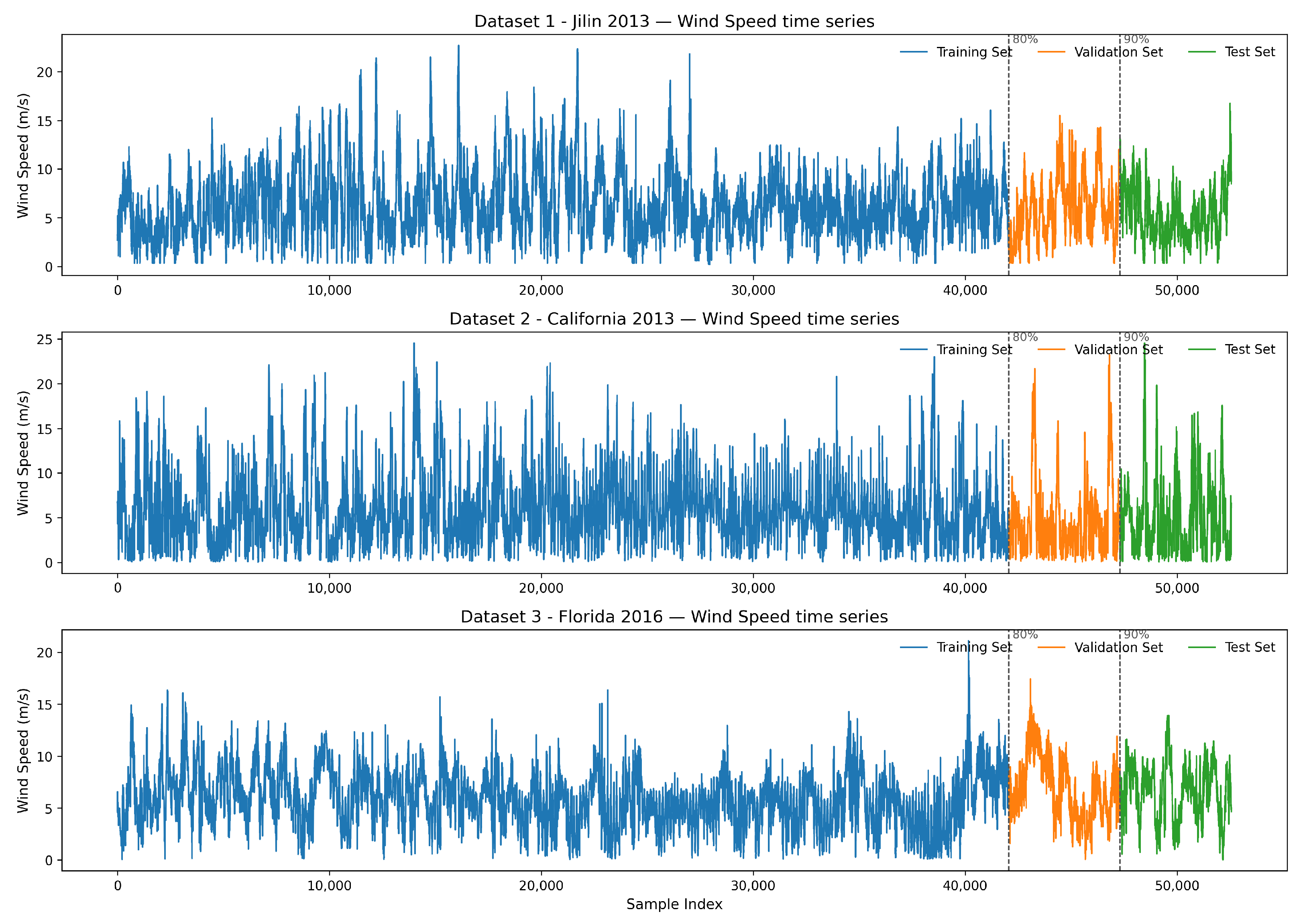
To mitigate the spectral leakage effect that may occur during the transition from the time domain to the time-frequency domain in Stationary Wavelet Transform (SWT), the dataset was constructed with a base sampling window that is an integer multiple of 24 h. When the sampling period is not an integer multiple of the signal period, spectral leakage can occur, leading to the loss of central frequency information due to improper truncation of the original signal. Therefore, each input sample in this study consists of a 48 h wind speed sequence, corresponding to 288 time steps, and is used to predict the wind speed for the 6th hour in the future. As shown in Figure 5, the dataset was divided into training, validation, and test sets in a ratio of 8:1:1. The training set was used to compute the loss for each batch and update model parameters via backpropagation. The validation set was used at the end of each epoch to evaluate the model’s validation loss, enabling the ReduceLROnPlateau scheduler to adjust the learning rate dynamically and the EarlyStopping mechanism to determine when to halt training to prevent overfitting. The test set was used only after the training process was completed to perform a one-time evaluation independent of training, and to compute performance metrics such as MAE, RMSE, and $R^2$, thereby objectively reflecting the generalization capability of the model.

3.2. Evaluation Metrics

To evaluate the performance of the proposed model, this study adopts four commonly used metrics: mean absolute error (MAE), root mean square error (RMSE), mean absolute percentage error (MAPE), and the coefficient of determination ($R^2$). The corresponding formulations are given as follows:

$$\mathrm{MAE}={\displaystyle \frac{1}{n}}\sum _{i=1}^n\left|y_i-{\widehat{y}}_i\right|$$

(13)

$$\mathrm{RMSE}=\sqrt{{\displaystyle \frac{1}{n}}\sum _{i=1}^n{\left(y_i-{\widehat{y}}_i\right)}^2}$$

(14)

$$\mathrm{MAPE}={\displaystyle \frac{1}{n}}\sum _{i=1}^n\left|{\displaystyle \frac{y_i-{\widehat{y}}_i}{y_i}}\right|\times 100\%$$

(15)

$$R^2=1-{\displaystyle \frac{{\displaystyle \sum _{i=1}^n{\left(y_i-{\widehat{y}}_i\right)}^2}}{{\displaystyle \sum _{i=1}^n{\left(y_i-\overline{y}\right)}^2}}}$$

(16)

where n is the number of samples, $y_i$ denotes the actual value, ${\widehat{y}}_i$ denotes the predicted value, and $\overline{y}$ is the mean of the actual values.

3.3. Establishment of the Proposed Model

To enhance the accuracy and stability of wind speed forecasting, this study develops a multi-feature-driven hybrid deep learning framework. The overall architecture consists of three main components: wind speed decomposition, multi-feature forecasting, and nonlinear fusion-based output prediction.

First, for the core variable—wind speed—the original time series is decomposed using the stationary wavelet transform (SWT) combined with a turbulence intensity calculation approach. And the empirical scaling factor for the low-frequency components here is selected as $1.3^{m-1}$, where m denotes the m-th level low-frequency component. The wavelet basis function selected is sym8, a member of the Symlet wavelet family, which possesses approximate symmetry. Such symmetric wavelets are capable of reducing phase distortion during signal reconstruction, which is particularly important for preserving the temporal features of non-stationary signals like wind speed. Moreover, sym8 exhibits high regularity (smoothness), effectively mitigating pseudo-Gibbs phenomena (e.g., edge oscillations) in wind speed decomposition, especially suitable for analyzing the continuous variation of wind profiles.

To comprehensively capture the uncertainty of wind speed across both large and small time scales, the SWT decomposition level is set to 8. The low-frequency components of the wind speed signal are used to estimate the multi-scale average wind speed, which reflects its long-term trend. Meanwhile, the squared difference between the actual and average wind speed is computed, and its low-frequency part is employed to estimate the mean squared deviation. Based on the turbulence intensity formulas at each decomposition level, the turbulence intensities across different time resolutions are derived. The resulting eight layers of average wind speed and turbulence intensity derived from Dataset 1 at different temporal scales are illustrated in Figure 6.

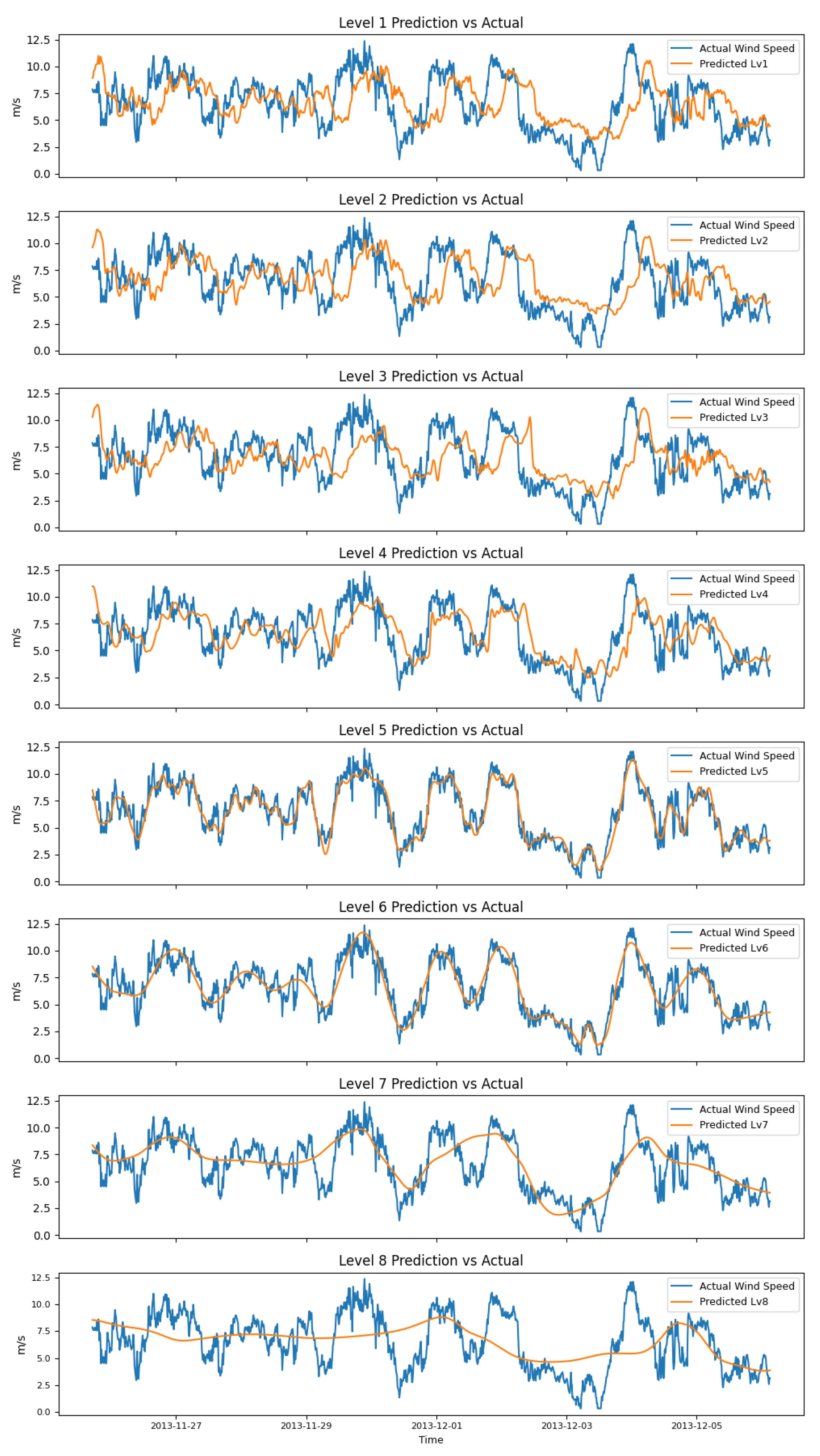
Subsequently, the eight groups of average wind speed and turbulence intensity sub-sequences, corresponding to different time scales, are fed into eight independently constructed LSTM models to perform wind speed forecasting at each respective scale. As a result, eight sets of wind speed predictions under different temporal resolutions are obtained. Figure 7 presents a comparison between the predicted wind speed values at each time scale and the actual wind speed on Dataset 1.

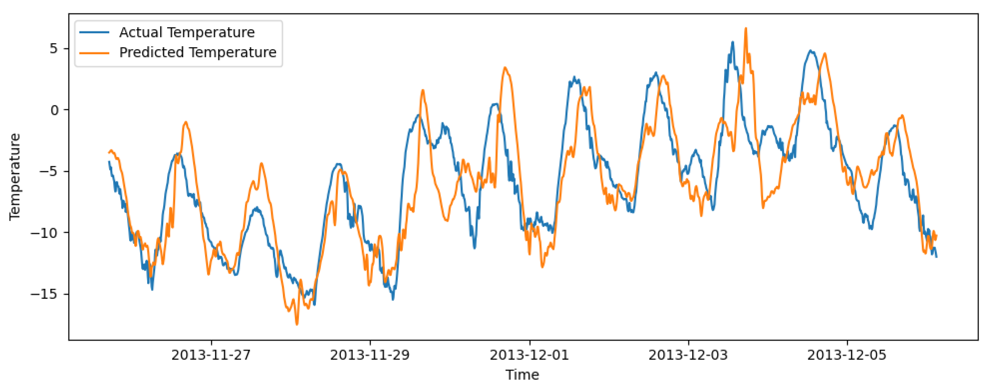
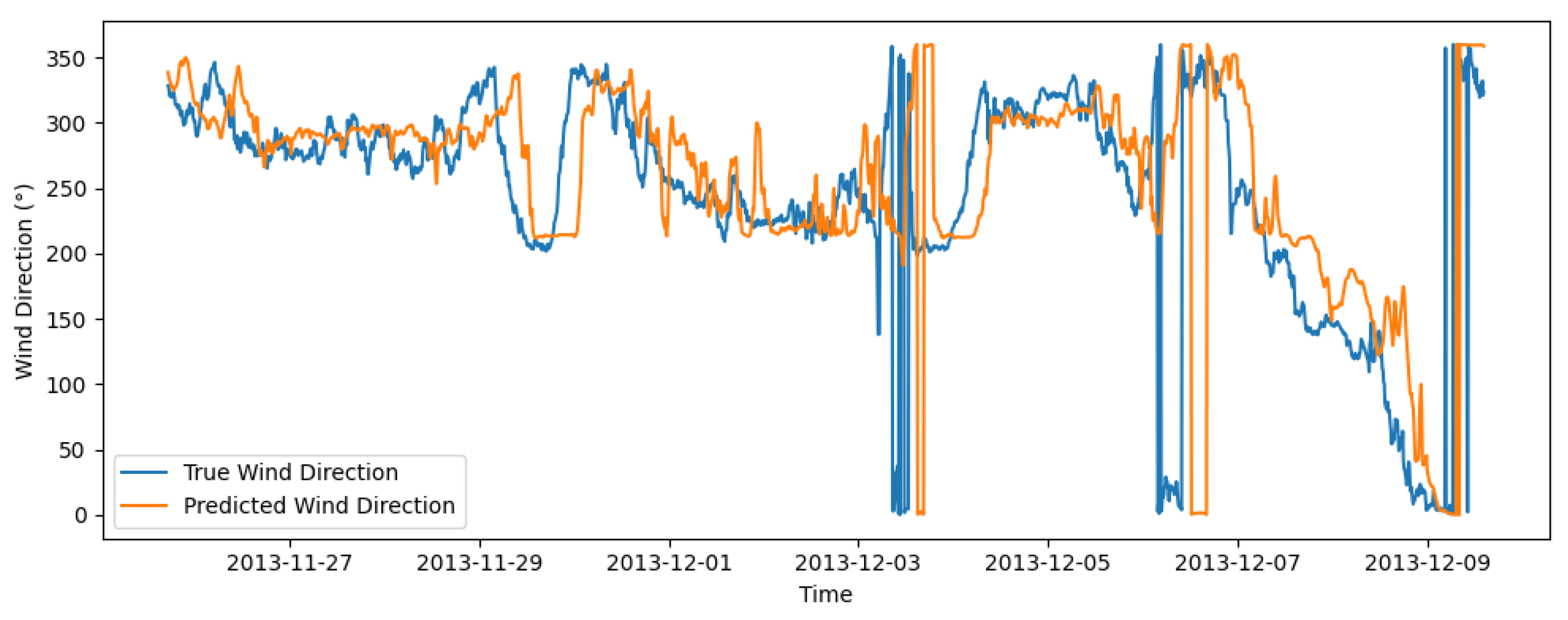
To further incorporate auxiliary information from external meteorological factors, the model simultaneously establishes prediction modules for atmospheric pressure, temperature, and wind direction. Specifically, the atmospheric pressure series is predicted using the WaveNet model to capture long-term dependencies and local convolutional features. As illustrated in Figure 8, the predicted and actual values of pressure on Dataset 1 are compared. The temperature series is modeled using a traditional LSTM network to capture temporal dependencies of temperature variations, with the prediction results on Dataset 1 shown in Figure 9. Considering the periodic characteristics of wind direction data, a TCN model is introduced for effective modeling. To address the periodicity, this study converts the wind direction angle $\theta$ into a two-dimensional vector representation $\left(\cos \right(\theta ),\sin (\theta \left)\right)$ prior to modeling, thereby preserving the continuity of the periodic data. These transformed features are fed into the TCN network, whose outputs are the predicted sine and cosine components of wind direction. Figure 10 shows the comparison between predicted and actual wind direction on Dataset 1; Figure 11a presents the scatter plot of predicted versus actual sine and cosine values of wind direction on Dataset 1, the line segments on the unit circle plot represent error vectors that start at each true wind direction point and point to the corresponding predicted wind direction, where the orientation of each arrow indicates whether the prediction is clockwise or counterclockwise relative to the true direction and the length and color of the arrow encode the magnitude of the angular error in degrees. Figure 11b shows the wind direction-prediction error distribution on Dataset 1.

A total of 12 predictive features are obtained from the above process, including 8 wind speed sub-component predictions and 4 meteorological variable predictions. Finally, all predicted features are collectively fed into a Transformer model, which leverages its self-attention mechanism to capture temporal dependencies and nonlinear relationships among multiple variables, thereby achieving effective feature fusion and the final wind speed prediction. The structure and parameter settings of each sub-model in the proposed model are shown in

Table 2. Proposed model structures and parameters.

Model	Structure	Parameters
LSTM for wind speed	Input layer	Shape: (288, 2)
	LSTM layer	Units: 64
	Dropout	Dropout rate: 0.1
	Fully Connection	Units: 1
WaveNet for presure	Residual Block	Layer number: 6
		Residual filters: 32
		Skip filters: 64
		Kernel size: 2
		Dilation rate: $2^{(m-1)}$
	Skip Connection Aggregation	Activation: ReLU
	Post-Aggregation Conv1D	Filters: 64
		Kernel size: 1
	Output Layer
LSTM for temperature	Input layer	Shape: (288, 1)
	LSTM layer 1	Units: 64
	Dropout 1	Dropout rate: 0.2
	LSTM layer 2	Units: 32
	Dropout 2	Dropout rate: 0.2
	Fully Connection	Units: 1
TCN for wind direction	Input Convolution Layer	Number of filters: 64
		Dilation rate: 1
		Kernel size: 5
	First Dilated Convolution Layer	Number of filters: 64
		Dilation rate: 1
		Kernel size: 5
	Second Dilated Convolution Layer	Number of filters: 128
		Dilation rate: 2
		Kernel size: 5
	Third Dilated Convolution Layer	Number of filters: 256
		Dilation rate: 4
		Kernel size: 5
	Time Feature Fully Connection	Input units: 2
		Hidden units: 16
		Activation: ReLU
		Dropout rate: 0.2
	Output Fully Connection	Fully Connection 1 units: 64
		Activation: ReLU
		Dropout rate: 0.2
		Fully Connection 2 units: 2
		Activation: Tanh
		$L^2$ normalization
Transformer for output	Encoder Layers	Number: 4
		Attention heads: 8
		FFN Dimension: 512
		Dropout: 0.1
	Feature Fusion Layer	Input Dim: 1536
		Hidden Units: 128
		Activation: ReLU
		Dropout: 0.1
	Output Layer	Fully Connection number: 2
		Activation: ReLU
		Dropout: 0.1

. This integrated framework combines multi-scale wind speed modeling with multi-source meteorological information modeling, and benefits from the global modeling capability of the Transformer architecture. As a result, it significantly improves the accuracy and generalization ability of the wind speed forecasting model.

At the output stage, the model was trained using the Adam optimizer (initial learning rate = 0.001, batch size = 64, maximum epochs = 100) with Mean Squared Error (MSE) loss. A ReduceLROnPlateau scheduler was applied to reduce the learning rate when validation loss plateaued, and gradient clipping (max-norm = 1.0) was used to improve stability. Early stopping with patience = 10 was employed, and the model with the lowest validation loss was selected for final evaluation. The hyperparameters were determined through manual trial-and-error guided by validation performance. All experiments were conducted on Ubuntu 20.04 with Python 3.8, CUDA 11.8, using a single NVIDIA RTX 4090 GPU (24 GB, NVIDIA Corporation, Santa Clara, CA, USA), a 16 vCPU Intel Xeon Gold 6430 processor (Intel Corporation, Santa Clara, CA, USA), and 120 GB RAM (Samsung Electronics Co., Ltd., Suwon, Republic of Korea).

4. Experimental Results and Analysis

4.1. Ablation Study and Results

To examine the contribution of each core component in the proposed hybrid integration model, ablation experiments were conducted by removing key modules individually. Specifically, Ablation I removes the turbulence intensity feature, feeding only the SWT-derived average wind speed subsequences into the eight LSTM sub-models. Ablation II removes SWT decomposition, directly inputting the raw wind speed series into a single LSTM. Ablation III excludes the independent air pressure branch, omitting WaveNet-predicted pressure features from the Transformer fusion. Ablation IV excludes the independent air temperature branch, omitting LSTM-predicted temperature features from the fusion stage. Ablation V removes the wind direction branch, omitting TCN-predicted direction features. In all cases, the Transformer fusion module is retained for consistency. The models are evaluated on Dataset 1 using MAE, RMSE, MAPE, and $R^2$.

To assess the statistical significance of performance differences between the proposed model and its ablation variants, the Wilcoxon signed-rank test is employed. This non-parametric paired test evaluates whether the median difference between two related samples is zero and is particularly suitable when the normality assumption is not satisfied.

In this study, the paired observations correspond to the prediction errors produced by the proposed model and each ablation variant. For each pair, the difference is defined as $D_i=e_a^i-e_p^i$, where $e_a^i$ and $e_p^i$ denote the prediction errors of the ablation model and the proposed model, respectively, for the i-th sample. Pairs with zero difference are excluded. The absolute differences $|D_i|$ of the remaining pairs are ranked, with tied values assigned average ranks. Then, the signed ranks are summed separately to obtain the positive and negative rank sums, denoted by $W^{+}$ and $W^{-}$, and the test statistic is defined as $W=min(W^{+},W^{-})$. The hypotheses are formulated as:

$$\begin{array}{c}\hfill H_0:median\left(D\right)=0\mathrm{vs}.H_1:median\left(D\right)\ne 0.\end{array}$$

Under the null hypothesis, for large samples, the test statistic defined as

$$Z={\displaystyle \frac{W-{\mu }_W}{{\sigma }_W}}\stackrel{L}{\to }N(0,1),$$

can be employed to compute the critical values of the test, where ${\mu }_W=n(n+1)/4$ and ${\sigma }_W=\sqrt{n(n+1)(2n+1)/24}$, with n denoting the number of nonzero differences. If the resulting p-value is less than the predefined significance level (e.g., $\alpha =0.05$), the null hypothesis is rejected, indicating that the performance difference between the baseline and the ablation variant is statistically significant.

The ablation results summarized in

Table 3. Ablation experiment results of the proposed model.

Model	MAE	RMSE	MAPE (%)	${\mathit{R}}^2$
The proposed model	0.5418	0.6940	14.88%	0.9161
Excluding turbulence intensity	0.5724	0.7404	17.09%	0.9045
Excluding SWT	1.5667	1.9524	51.77%	0.3361
Excluding pressure	0.5586	0.7110	16.81%	0.9119
Excluding temperature	0.5591	0.7094	16.02%	0.9124
Excluding direction	0.5502	0.7044	16.10%	0.9136

demonstrate that each component contributes to the predictive performance of the proposed model. In particular, removing SWT decomposition causes the most severe degradation, confirming its central role in capturing multi-scale wind speed patterns. Excluding turbulence intensity, pressure, temperature, or direction also leads to significant increases in error, though to a lesser extent.

The Wilcoxon signed-rank test results in

Table 4. Wilcoxon signed-rank test results of the proposed model against its ablation variants.

Compared to Proposed	Paired Sample Size	Wilcoxon W	p-Value (Raw)	p-Value (Holm)	Significant?
Excluding turbulence intensity	5005	5,635,910.5	$8.175\times {10}^{-10}$	$3.270\times {10}^{-9}$	Yes
Excluding SWT	5005	1,167,178	0	0	Yes
Excluding pressure	5005	5,715,100.5	$8.012\times {10}^{-8}$	$2.404\times {10}^{-7}$	Yes
Excluding temperature	5005	5,790,223.5	$3.621\times {10}^{-6}$	$7.242\times {10}^{-6}$	Yes
Excluding direction	5005	6,011,215.5	$1.350\times {10}^{-2}$	$1.350\times {10}^{-2}$	Yes

The column p-value (Raw) reports the unadjusted significance level. p-value (Holm) represents the Holm-adjusted p-values for multiple comparisons. The Significant? column indicates whether the result is statistically significant at the $\alpha =0.05$ level.

further validate these findings. All ablation variants show statistically significant differences from the proposed model ($p<0.05$ after Holm adjustment), indicating that the performance gains are not due to random variation. Among the auxiliary features, turbulence intensity exerts the strongest influence, while pressure, temperature, and direction also provide complementary improvements. Together, these results confirm that each module in the hybrid integration framework is indispensable for achieving superior forecasting accuracy.

4.2. Comparative Experiments and Results

To evaluate the predictive performance of the proposed hybrid ensemble model, four sets of comparative experiments were conducted: (1) comparison with representative single deep learning models for wind speed forecasting to demonstrate the necessity of model integration; (2) comparison with classical signal decomposition-based AI models to highlight the superiority of the proposed decomposition strategy based on turbulence intensity and stationary wavelet transform (SWT); (3) comparison with linearly optimized ensemble models to validate the advantage of the Transformer-based nonlinear dynamic fusion mechanism; and (4) comparison with single-feature wind speed-prediction models to emphasize the importance of incorporating multi-scale and multivariate meteorological features. The experimental results across three datasets are shown in

Table 5. Performance comparison of different wind speed-forecasting models across three datasets.

Dataset	Experiment	Model	MAE	RMSE	MAPE	${\mathit{R}}^2$
Dataset 1	Proposed	Proposed Model	0.5418	0.6940	14.88%	0.9161
	Comparison I	LSTM	1.6562	2.0725	52.34%	0.2518
		Transformer	1.6397	2.0410	55.35%	0.2744
		CNN1dLSTM	1.6548	2.0423	56.07%	0.2735
		TCN	1.8560	2.2142	66.00%	0.1461
		GRU	1.6186	2.0005	53.56%	0.3029
		BiLSTM	1.6223	2.0022	53.97%	0.3017
	Comparison II	STL-LSTM	1.5772	2.1461	47.95%	0.1977
		VMD-Transformer	0.7265	0.9359	22.50%	0.8474
	Comparison III	WOA linear combination	0.5783	0.7402	16.80%	0.9045
		CSA linear combination	0.7964	0.9835	26.44%	0.8315
	Comparison IV	Single-Feature SWT-LSTM	0.5924	0.7621	16.29%	0.8980
Dataset 2	Proposed	Proposed Model	0.9337	1.2684	43.24%	0.8994
	Comparison I	LSTM	2.6587	3.4497	144.64%	0.2561
		Transformer	2.7302	3.5021	152.63%	0.2333
		CNN1dLSTM	2.6798	3.4837	140.84%	0.2414
		TCN	3.0688	3.8486	175.88%	0.0741
		GRU	2.7175	3.4682	154.18%	0.2481
		BiLSTM	2.5637	3.4486	127.13%	0.2566
	Comparison II	STL-LSTM	2.4885	3.4024	124.26%	0.2764
		VMD-Transformer	0.9666	1.3206	40.40%	0.8910
	Comparison III	WOA linear combination	1.0244	1.3820	51.23%	0.8806
		CSA linear combination	1.5650	1.9144	99.56%	0.7709
	Comparison IV	Single-Feature SWT-LSTM	1.0358	1.3963	51.87%	0.8781
Dataset 3	Proposed	Proposed Model	0.4639	0.6596	11.61%	0.9367
	Comparison I	LSTM	1.5474	1.9677	41.43%	0.4368
		Transformer	1.5545	1.9662	44.40%	0.4376
		CNN1dLSTM	1.5757	1.9975	42.59%	0.4196
		TCN	1.6840	2.1247	44.03%	0.3433
		GRU	1.4846	1.8732	38.62%	0.4895
		BiLSTM	1.4414	1.8715	34.92%	0.4905
	Comparison II	STL-LSTM	1.4070	1.8238	44.20%	0.5161
		VMD-Transformer	0.7366	0.9515	14.88%	0.8683
	Comparison III	WOA linear combination	0.5304	0.7140	13.08%	0.9258
		CSA linear combination	1.4744	1.8019	40.78%	0.5277
	Comparison IV	Single-Feature SWT-LSTM	0.5276	0.7138	12.50%	0.9259

Bold values indicate that the corresponding model achieved the best performance on that metric.

.

To ensure a smooth flow and concise presentation of the main text, the complete visualization results on Dataset 1, which are representative of the overall performance, are presented in Figure 12, Figure 13, Figure 14, Figure 15 and Figure 16. For Dataset 2 and Dataset 3, only the most representative figures are shown in the main text (Figure 17 and Figure 18), with the remaining detailed visualizations provided in Appendix A. These additional figures represent repeated experiments of our proposed model on different datasets and are also crucial for verifying its performance.

4.2.1. Comparison Experiment I: Comparison with Single Models

To validate the effectiveness of the proposed hybrid model that integrates multi-scale turbulence intensity features with a Transformer-based framework, several representative single deep learning models—including LSTM, CNN1dLSTM, Transformer, TCN, GRU, and BiLSTM—were selected for comparative analysis. As shown in Table 5, the proposed model achieves substantial improvements in all forecasting metrics compared to individual models. On average over the three datasets, it reduces the error metrics by 67.8% in MAE, 65.6% in RMSE, and 71.9% in MAPE, while increasing the coefficient of determination $R^2$ by 267.1%. These results strongly highlight the superiority of the proposed hybrid ensemble model over individual deep learning approaches in wind speed forecasting.

The visual comparison further validates these findings. Let us focus on the comparison of the prediction curves in subfigures (a) and (b) of Figure 12, Figure 17 and Figure 18, which correspond to the three datasets. On Dataset 1, the proposed model not only closely follows the long-term trend of the actual wind speed but also accurately captures most short-term fluctuations. It demonstrates satisfactory reproduction of both peaks and troughs, with only slight lag and amplitude smoothing observed at a few sharp transitions. In contrast, the single models presented in subfigure (b) exhibit evident phase lags and amplitude distortions. On Dataset 2, where the actual wind speed reaches higher values (up to nearly 14 m/s) and more intense fluctuations are present, the superiority of the proposed model is even more pronounced. Single models generally fail to capture the steep peaks and tend to underestimate rapid rises in wind speed. On Dataset 3, where wind speeds are more stable (2–10 m/s), the proposed model still provides the closest tracking of the ground truth, while single models show larger deviations in the medium ranges. Overall, these results highlight the robustness and generalization ability of the proposed hybrid ensemble model across diverse climatic conditions.

4.2.2. Comparison Experiment II: Comparison with Data Preprocessing + AI Models

To further explore the performance differences between AI models that integrate multivariate meteorological data dynamic modeling and traditional data-preprocessing techniques, this study selects two classical preprocessing-based models—STL-LSTM and VMD-Transformer—as benchmarks. As shown in Table 5, compared with STL-LSTM, the proposed model reduces MAE, RMSE and MAPE by approximately $65.05\%$, $64.74\%$ and $69.3\%$, respectively, and improves $R^2$ by about $223.42\%$ on average over the three datasets. In comparison with the more advanced VMD-Transformer model, the proposed model achieves reductions of about $21.95\%$ in MAE, $20.16\%$ in RMSE and $16.27\%$ in MAPE, while increasing $R^2$ by $5.64\%$ on average over the three datasets. As illustrated in subfigure (c) of Figure 12, Figure 17 and Figure 18, the hybrid model produces forecast curves with less delay compared to single models. On Dataset 1, the VMD-Transformer effectively eliminates high-frequency noise and restores the overall trend, but it still deviates from the ground truth in finer details (e.g., near sample 150 and 300). Due to the smoothing effect of STL, STL-LSTM yields excessively flat prediction curves, resulting in poor amplitude estimation and a pronounced phase shift. On Dataset 2, the advantage of the proposed model becomes clearer: the high-frequency noise is more prominent in this dataset, so the VMD-Transformer demonstrates partial improvements but still suffers from detail mismatches, while STL-LSTM exhibits even stronger over-smoothing and severe phase delays. For Dataset 3, the relatively smoother wind speed series reduces the severity of noise, making the limitations of STL-LSTM less visible. Nevertheless, the hybrid model continues to provide superior alignment with the observed values. These findings indicate that the proposed multivariate dynamic prediction strategy can more effectively extract underlying meteorological dynamics than traditional preprocessing-based methods, thus improving both accuracy and stability across datasets.

4.2.3. Comparison Experiment III: Comparison with AI + Linear Combination Optimization Models

In this study, the proposed wind speed decomposition and multi-feature forecasting modules were retained, while only the final Transformer-based nonlinear fusion component was replaced with traditional optimization algorithms—WOA and CSA—for linear combination of outputs. As shown in Table 5, compared with the WOA-based linear combination model, the proposed model achieves reductions of approximately $9.23\%$, $7.36\%$, and $12.75\%$ in MAE, RMSE, and MAPE, respectively, while improving $R^2$ by about $1.53\%$ on average over the three datasets. When compared with the CSA-based linear combination model, MAE, RMSE, and MAPE decrease by $46.95\%$, $42.19\%$, and $57.27\%$, respectively, and $R^2$ increases by $34.78\%$ on average over the three datasets. Furthermore, it is noteworthy that even with a linear combination strategy, both models in this experiment outperform all models in Experiments I and II in terms of forecasting performance. This further validates the superiority of the proposed wind speed-decomposition method based on turbulence intensity and SWT, as well as the multi-feature parallel modeling framework. As depicted in subfigure (d) of Figure 12, Figure 17 and Figure 18, both models in Experiment III generate smoother forecasting curves than those of the single and preprocessing-based models, while also capturing the wind speed trend effectively. The WOA-based model tends to slightly underestimate peak values (e.g., around sample 400–420) but responds quickly to turning points. In contrast, the CSA-based model produces slightly elevated troughs (e.g., around samples 80 and 500) while maintaining smoothness, resulting in better overall reconstruction of peak and valley structures. These findings suggest that, compared to traditional linear combination fusion methods, the self-attention mechanism of the Transformer can more effectively achieve nonlinear dynamic fusion of multi-model outputs.

4.2.4. Comparison Experiment IV: Comparison with Single-Feature SWT-LSTM Model

To evaluate the effectiveness of the proposed parallel modeling strategy that incorporates multi-scale structures and multiple meteorological features, a comparative experiment was conducted against a baseline model using the same SWT- and turbulence-intensity-based wind speed-decomposition method combined with LSTM, but limited to a single temporal scale and a single wind speed feature without incorporating other meteorological variables. As shown in Table 5, the proposed model achieves reductions of approximately $10.16\%$, $8.56\%$, and $10.8\%$ in MAE, RMSE, and MAPE, respectively, while the coefficient of determination ($R^2$) increases by about $1.87\%$ on average over the three datasets. The time-series curves of actual and predicted wind speeds are illustrated in subfigure (e) of Figure 12, Figure 17 and Figure 18. The SWT-LSTM model, which relies solely on wind speed as input, produces smoother curves than single deep learning models. However, it fails to capture the fine-tuning effects of other influencing factors such as air pressure, temperature, and wind direction on wind speed dynamics. This result indicates that the proposed parallel modeling approach, which incorporates multi-scale structure and multiple meteorological features, can more effectively extract complex temporal patterns of wind speed sequences and thus improve the overall forecasting performance. Furthermore, both models in Experiment IV outperform the STL-LSTM and VMD-Transformer models in Experiment II, demonstrating that the proposed decomposition method based on turbulence intensity and SWT is superior to traditional wind speed decomposition techniques.

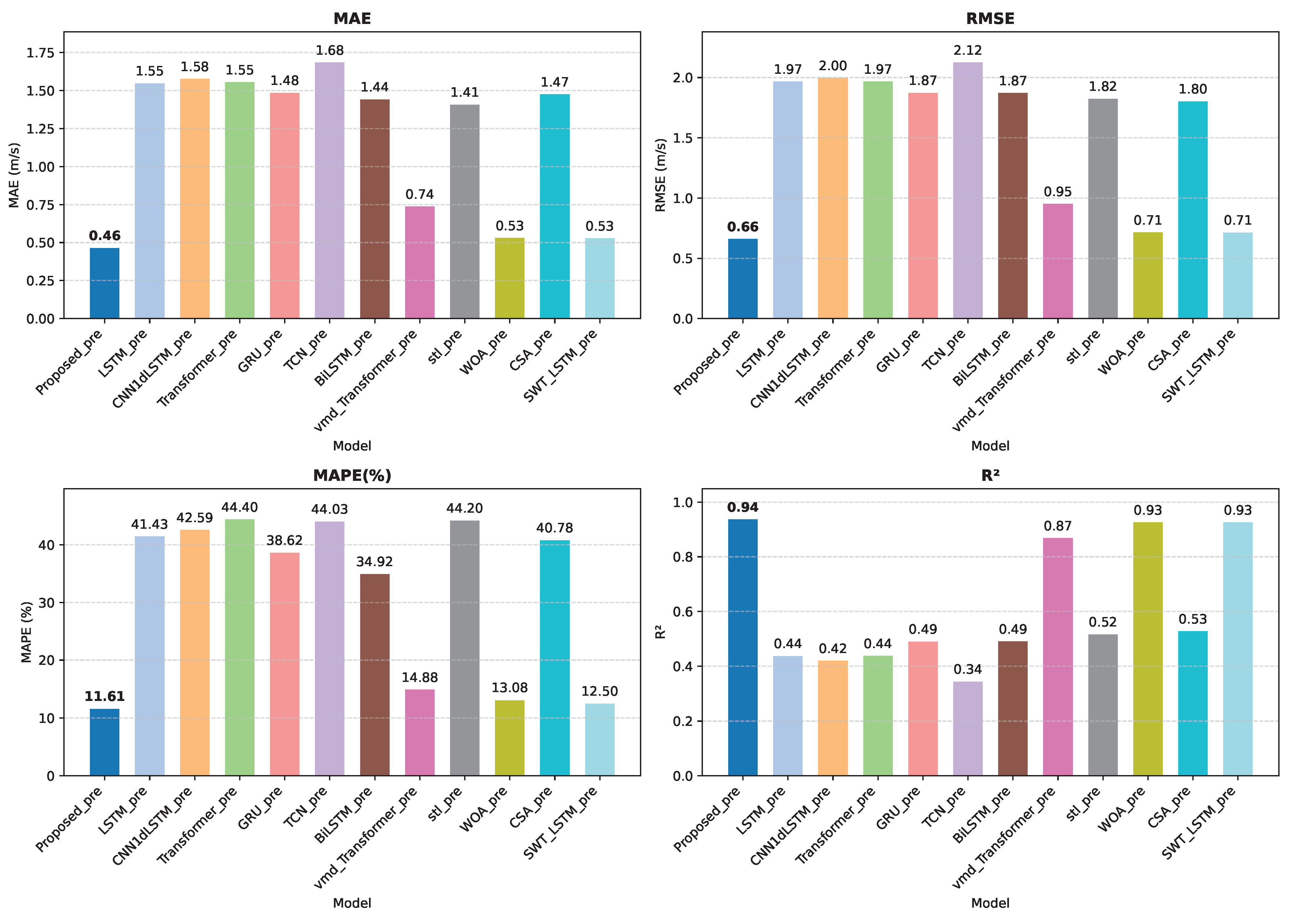
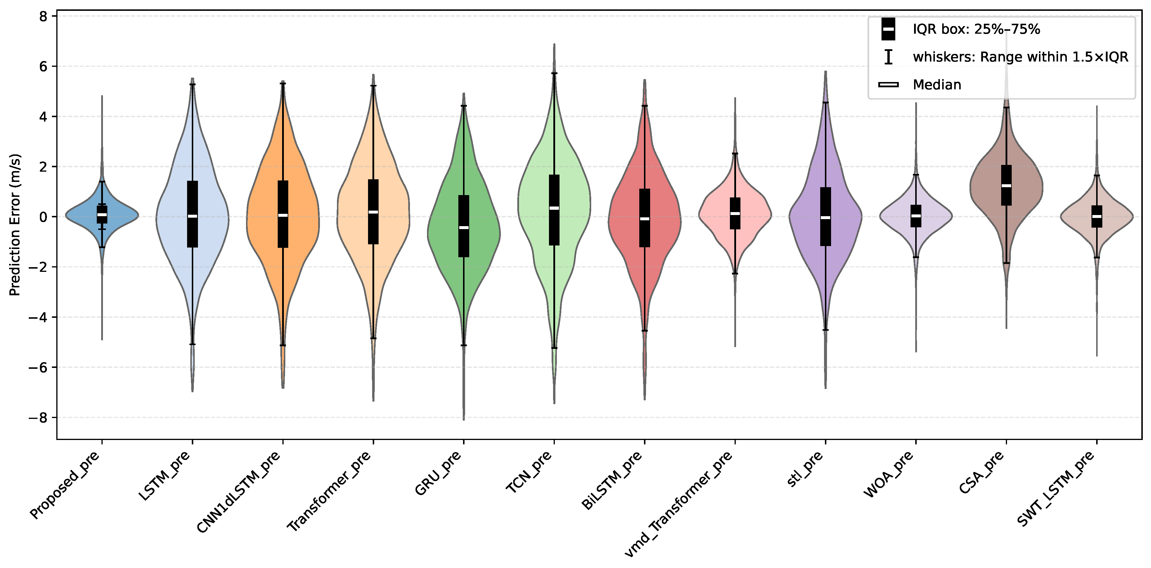
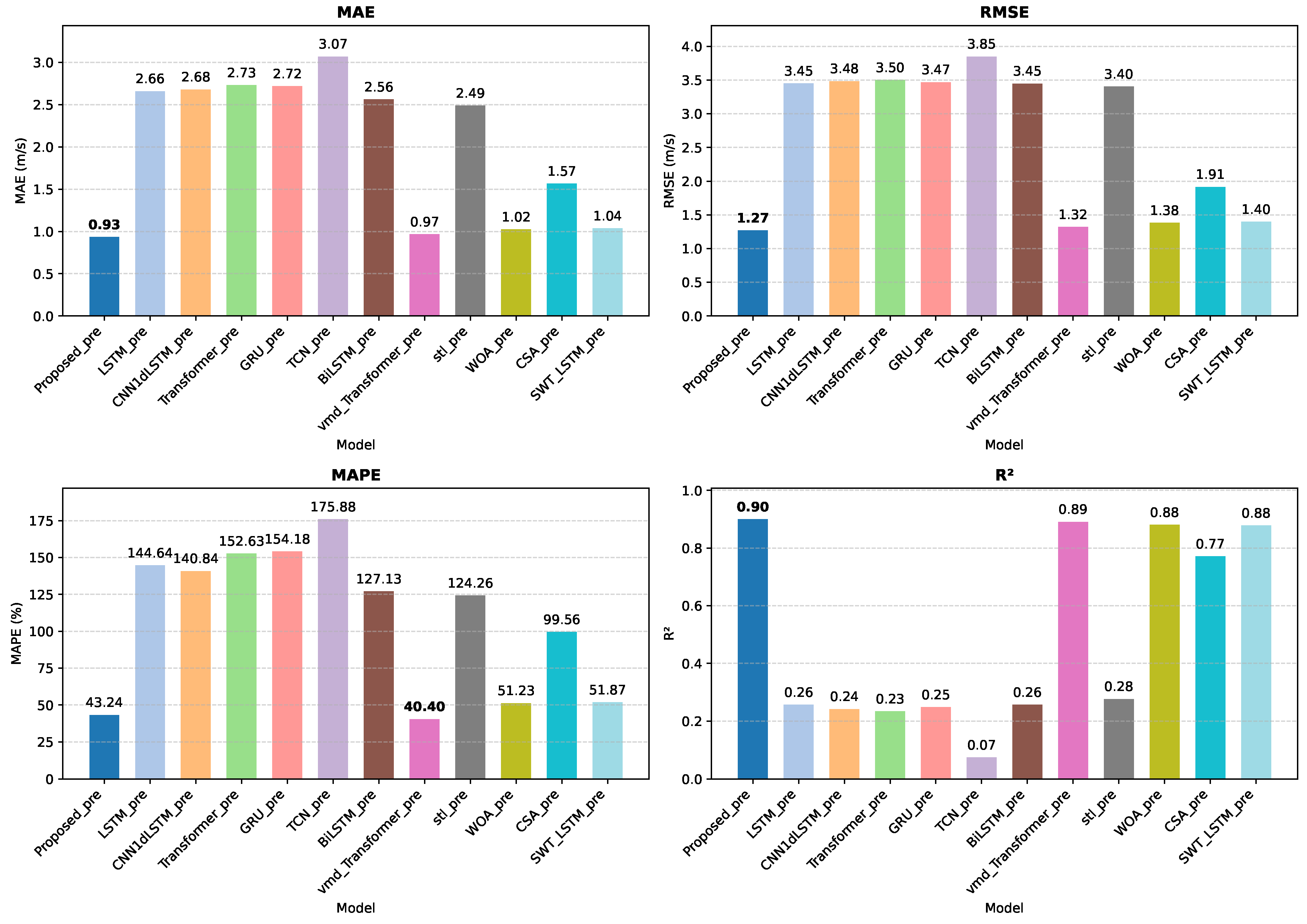
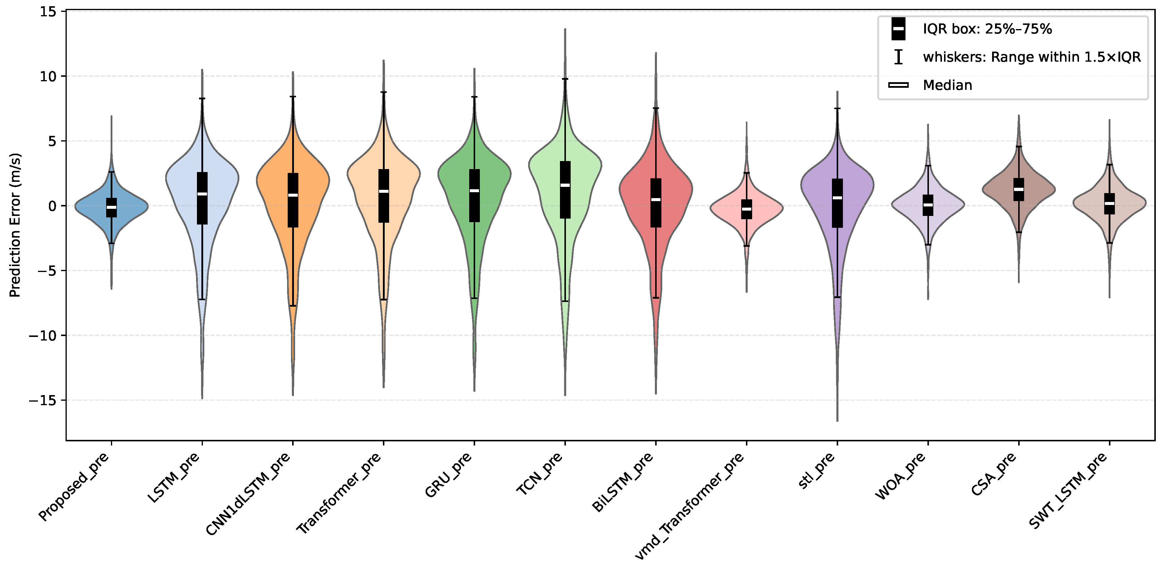
As shown in Figure 13, the proposed wind speed-forecasting model achieves the best performance across all four evaluation metrics, with the best-performing model in each metric highlighted in bold. This conclusion is further supported by the other visualization results. The violin plot presented in the Figure 14 illustrates the distribution of prediction errors for all models. Among them, the proposed hybrid ensemble model exhibits the most desirable characteristics: its median prediction error is nearly zero, indicating minimal systematic bias; its interquartile range (IQR) is the narrowest, suggesting high stability and consistency in forecasts; and its error tails are short and symmetric, with very few extreme deviations beyond ±2 m/s. In contrast, most single deep learning models show wider IQRs and more pronounced tails, reflecting larger fluctuations and higher occurrence of extreme errors. Notably, TCN and STL display the longest tails, with occasional errors exceeding ±8 m/s, indicating lower reliability under volatile conditions. Models based on signal decomposition and optimization achieve better control over extreme errors and have moderately narrow IQRs, but still fall short of the compact and symmetric error distribution achieved by the proposed model. Overall, the proposed method demonstrates superior predictive accuracy, robustness, and error stability, validating the effectiveness of multi-resolution turbulence features, Transformer-based dynamic fusion, and ensemble learning strategies in wind speed forecasting.

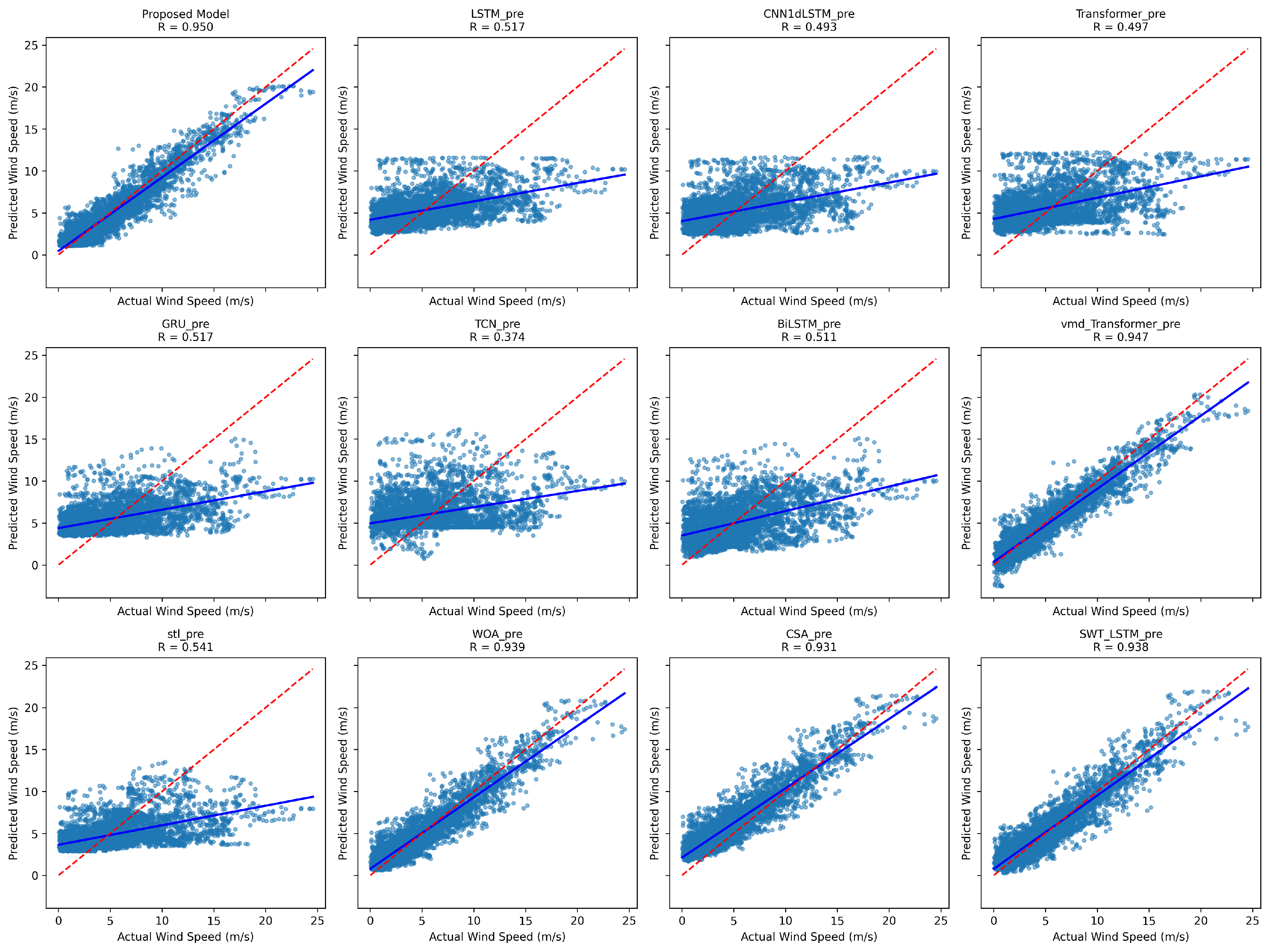
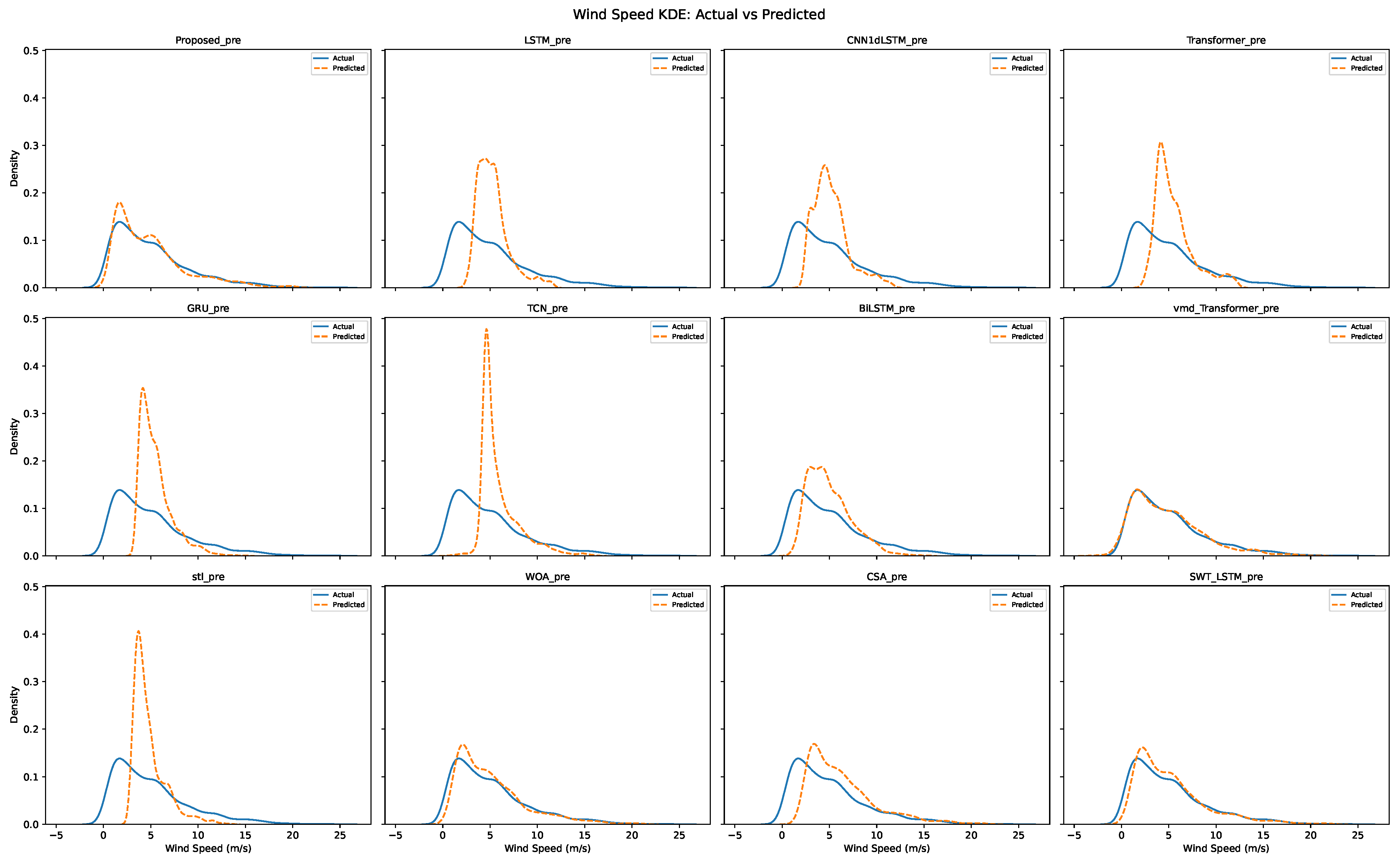
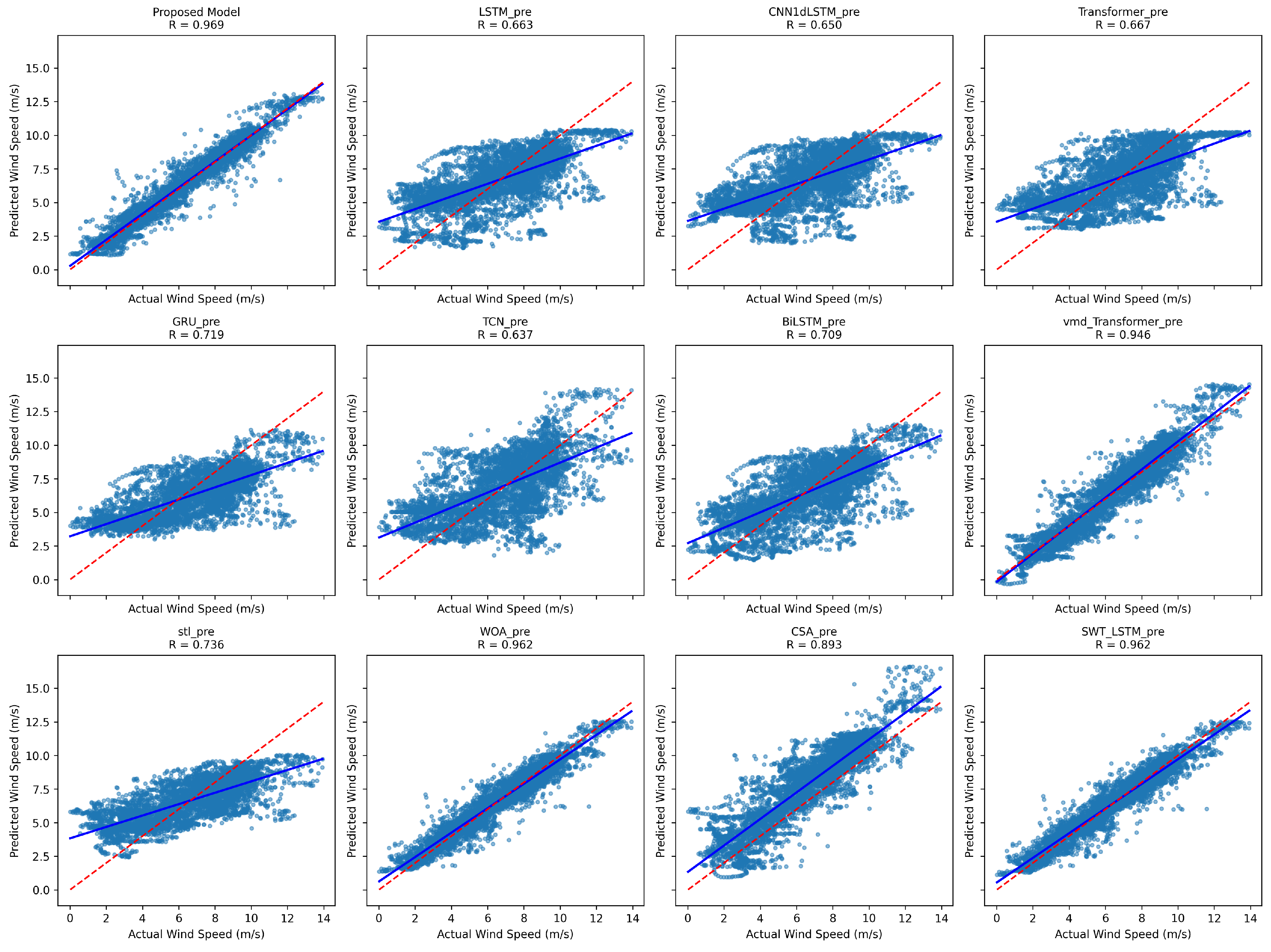
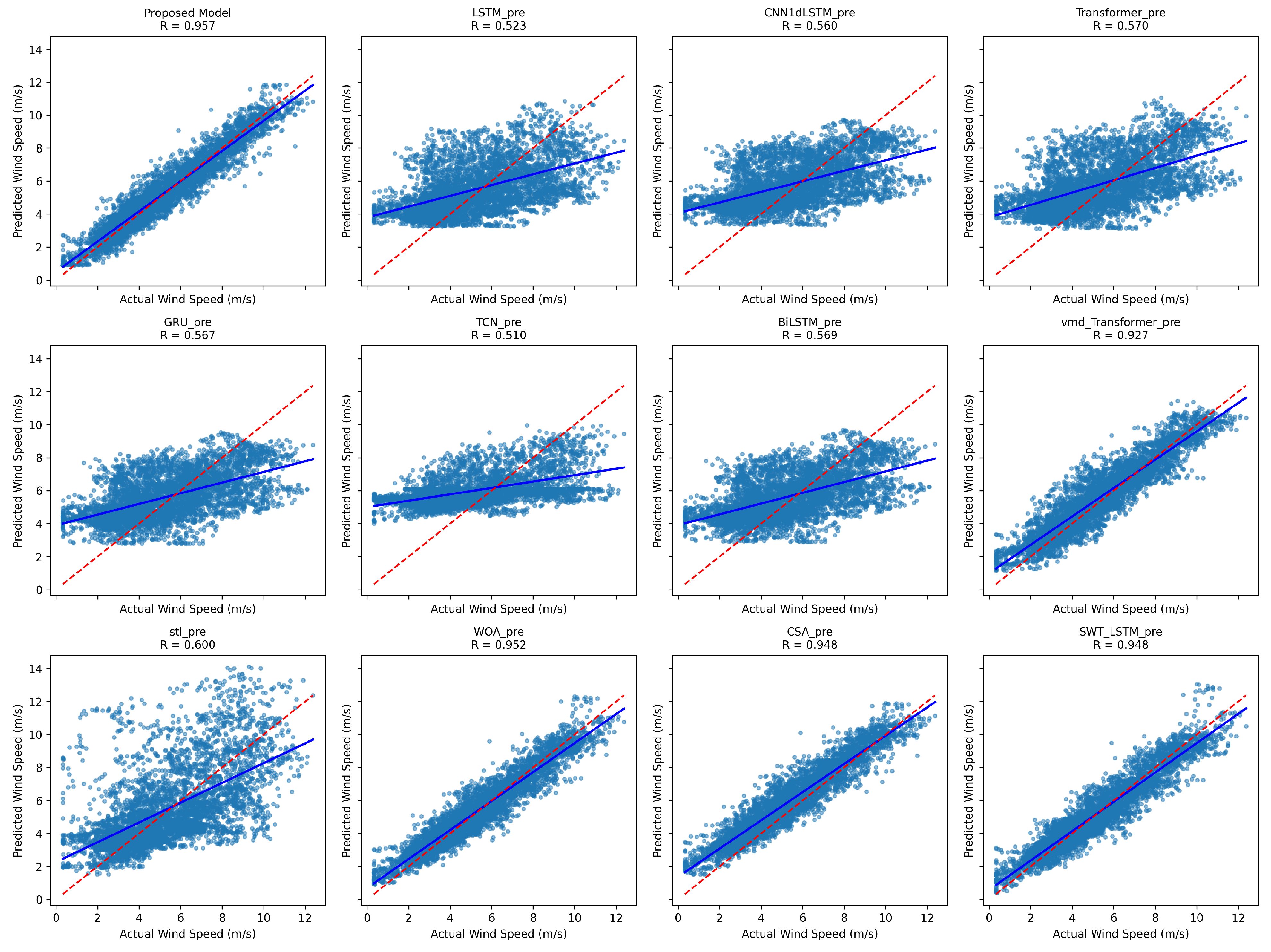
Figure 15 presents the scatter plots of predicted versus actual wind speeds for all models. The proposed model demonstrates a high concentration of scatter points along the diagonal, with its regression line nearly overlapping the red reference line, indicating both minimal systematic bias and a strong linear agreement with the true values over the entire sample range. In contrast, the scatter clouds of single deep learning models are more dispersed, with regression lines exhibiting slopes less than one. This suggests a common tendency among these models to overestimate low wind speeds and underestimate high wind speeds. The two ensemble models based on linear weight optimization (WOA and CSA) achieve a scatter distribution comparable to the proposed model around the diagonal. However, they show slight overestimation or underestimation in the extreme high-speed range (above 12 m/s), as evidenced by points deviating upward or downward from the ideal line. The single-feature SWT-LSTM model also exhibits a fitting performance close to that of the proposed model, but its regression line tends to slightly overestimate low-speed regions and underestimate high-speed ones. This indicates that while SWT-based decomposition offers smoothness, it may compromise some fine-grained dynamic details necessary for accurate forecasting. The kernel density estimates in Figure 16 compare the predicted wind speed distributions of twelve models with the actual wind speed distribution. The proposed model shows the closest alignment with the true distribution, accurately capturing both the primary peaks and tail characteristics.

4.2.5. Analysis of Training Time

In addition to model performance, computational efficiency is also an important consideration. We calculated and recorded the average training time of each model over six runs, and further averaged the results across the three datasets to eliminate the influence of data variability. As shown in

Table 6. Training time comparison of different models (unit: seconds).

Model	Training Time (s)	Model	Training Time (s)
proposed	2382.34	TCN	85.61
WOA linear combination	2153.89	GRU	350.38
CSA linear combination	2132.42	BiLSTM	1625.8
STL-LSTM	503.41	LSTM	27.03
VMD-Transformer	442.71	CNN1dLSTM	24.59
SWT-LSTM	1436.28	Transformer	58.91

, the results indicate that single deep learning models such as LSTM and TCN require relatively short training times due to their simple structures, which involve neither complex preprocessing steps nor multi-model integration. Models incorporating data-preprocessing techniques, such as STL-LSTM and VMD-Transformer, exhibit longer training times because the additional preprocessing introduces extra computational overhead. The Single-Feature SWT-LSTM, which includes a data-decomposition step, requires more time than single models but less than more sophisticated composite models that involve multi-feature parallel modeling. Our proposed model and the linear combination output model record the longest training times but also deliver the best performance. Notably, the linear output strategy with optimization algorithms requires slightly less time than the Transformer-based fusion output strategy, primarily due to its smaller number of parameters, differences in convergence strategy, and simpler architecture. Overall, considering the trade-off between performance and training time, the training time of our proposed model is reasonable.

5. Conclusions

To enhance the accuracy and stability of short- and medium-term wind speed forecasting, this study proposes a forecasting framework that integrates multi-resolution turbulence intensity features with a hybrid deep neural network architecture. Comprehensive experimental results demonstrate that the proposed model achieves significant improvements across multiple evaluation metrics, particularly showing superior adaptability and robustness in capturing high-frequency fluctuations and extreme values.

From a structural perspective, the integration of Stationary Wavelet Transform (SWT) and turbulence intensity-extraction modules enables multi-scale dynamic feature representation, allowing subsequent neural sub-models to capture both the trend and stochasticity of wind speed at varying temporal resolutions. In particular, the introduction of turbulence intensity provides an effective quantification of wind speed non-stationarity. Experimental evidence suggests that this feature significantly contributes to the prediction accuracy, especially during periods of sharp wind fluctuations.

In terms of predictive model design, three distinct architectures—LSTM, WaveNet, and TCN—are employed to model the coupling sequences between wind speed–turbulence and auxiliary meteorological variables at different scales. These models collaboratively extract informative features from both spatial locality and temporal dependency perspectives. Finally, a Transformer-based self-attention mechanism is used for feature fusion, which overcomes the limitations of traditional linear weighted summation by enabling nonlinear and adaptive aggregation of multi-source outputs. The experimental results indicate that the proposed method demonstrates outstanding accuracy and stability in mid-term wind speed prediction, achieving a MAE of 0.6465, RMSE of 0.8740, MAPE of $23.24\%$ and a coefficient of determination ($R^2$) of 0.9174 on average over the three datasets, suggesting strong potential for engineering applications.

Comparative experiments further validate the performance advantages of the proposed approach. Compared to typical single deep learning models (LSTM, CNN1d-LSTM, Transformer, TCN, GRU, BiLSTM), on average over the three datasets, the proposed model achieves over $65\%$ reductions in MAE and RMSE, and an improvement of more than $267\%$ in $R^2$, demonstrating the effectiveness of the hybrid ensemble strategy. Furthermore, in contrast to conventional preprocessing–AI model combinations such as STL-LSTM and VMD-Transformer, the proposed framework reduces MAE and RMSE by approximately $43\%$, and increases $R^2$ by $115\%$ on average over the three datasets, highlighting the advantages of dynamic multi-variable prediction. Additionally, when compared with output-combination methods using traditional optimization algorithms (e.g., WOA, CSA), the proposed model consistently outperforms across all metrics, confirming the effectiveness of the Transformer-based nonlinear fusion strategy.

Based on the wind speed-forecasting framework proposed in this study, several strategic approaches can be adopted to adapt the model to new locations. First, the multi-resolution decomposition mechanism of the Stationary Wavelet Transform (SWT) naturally accommodates different wind regimes. Second, the Transformer-based fusion mechanism, with its attention weights, can dynamically adjust the contributions of different features according to varying geographical and climatic conditions, thereby autonomously adapting to the relationships between meteorological factors and wind speed at different sites and ensuring strong transferability. Although the outstanding performance of the proposed model on three datasets from distinct geographical and climatic contexts already demonstrates its robustness, further adaptation strategies may be required when applying the model to entirely new locations. For such cases, a two-stage adaptation strategy can be employed. In the first stage, limited fine-tuning with a small amount of local data can be conducted, for instance by fine-tuning the parameters of SWT (e.g., wavelet basis functions and decomposition levels) to optimally capture the dominant fluctuation characteristics of local wind patterns. In the second stage, a continual learning mechanism can be established to progressively incorporate new data and adapt to evolving environmental conditions.

Despite the promising results in model design and forecasting accuracy, several future directions warrant further investigation:

(1)

Expansion of input features: Currently, the model focuses primarily on wind speed and turbulence intensity. Future research could incorporate additional meteorological variables such as boundary layer height, cloud cover, and humidity to improve sensitivity to complex climatic drivers.

(2)

Hyperparameter tuning approach: Some hyperparameters of the deep learning model were determined through empirical settings or trial-and-error methods under the guidance of validation performance, which makes it difficult to ensure that the global optimum is achieved. In future research work, we plan to explore more systematic and efficient hyperparameter optimization strategies, including Bayesian optimization and meta-heuristic algorithms such as particle swarm optimization and genetic algorithms, so as to further improve the model performance.

(3)

Fusion strategy optimization: Although the Transformer mechanism shows strong performance in feature fusion, its parameter redundancy and computational cost remain concerns. Lightweight attention mechanisms (e.g., Performer, Linformer) could be explored to retain accuracy while reducing training overhead.

(4)

Extreme wind event forecasting: While the model performs well overall, its accuracy in predicting sudden gusts or extreme wind events needs further enhancement. Future efforts may involve integrating extreme value theory or imbalanced learning techniques to improve early-warning performance under extreme conditions.

In conclusion, this study presents a feasible and effective approach for constructing a multi-scale wind speed-forecasting system with deep feature-extraction capabilities. Future research will focus on feature enrichment, multi-site adaptability, fusion optimization, and extreme event forecasting, thereby facilitating the deployment of the proposed model in real-world wind power systems.

References

1. Gsella, A.; de Meij, A.; Kerschbaumer, A.; Reimer, E.; Thunis, R.; Cuvelier, C. Evaluation MM5, WRF and TRAMPER meteorology over the complex terrain of the Po Valley, Italy. Atmos. Environ. 2014, 89, 797–806. [Google Scholar] [CrossRef]
2. Di, Z.; Ao, J.; Duan, Q.; Wang, J.; Gong, W.; Shen, C.; Gan, Y.; Liu, Z. Improving WRF model turbine-height wind-speed forecasting using a surrogate- based automatic optimization method. Atmos. Res. 2019, 226, 1–16. [Google Scholar] [CrossRef]
3. Chen, Y.; He, Z.; Shang, Z.; Li, C.; Li, L.; Xu, M. A novel combined model based on echo state network for multi-step ahead wind speed forecasting: A case study of NREL. Energy Convers. Manag. 2019, 179, 13–29. [Google Scholar] [CrossRef]
4. Ghofrani, M.; Arabali, A.; Etezadi-Amoli, M.; Fadali, M.S. Smart Scheduling and Cost-Benefit Analysis of Grid-Enabled Electric Vehicles for Wind Power Integration. IEEE Trans. Smart Grid 2014, 5, 2306–2313. [Google Scholar] [CrossRef]
5. Cadenas, E.; Rivera, W.; Campos-Amezcua, R.; Heard, C. Wind Speed Prediction Using a Univariate ARIMA Model and a Multivariate NARX Model. Energies 2016, 9, 109. [Google Scholar] [CrossRef]
6. Latimier, R.L.G.; Le Bouedec, E.; Monbet, V. Markov switching autoregressive modeling of wind power forecast errors. Electr. Power Syst. Res. 2020, 189, 106641. [Google Scholar] [CrossRef]
7. Wang, J.; Zhou, Q.; Jiang, H.; Hou, R. Short-Term Wind Speed Forecasting Using Support Vector Regression Optimized by Cuckoo Optimization Algorithm. Math. Probl. Eng. 2015, 2015, 619178. [Google Scholar] [CrossRef]
8. Ren, Y.; Suganthan, P.N.; Srikanth, N. A Novel Empirical Mode Decomposition with Support Vector Regression for Wind Speed Forecasting. IEEE Trans. Neural Networks Learn. Syst. 2014, 27, 1793–1798. [Google Scholar] [CrossRef]
9. Wang, Y.; Wang, J.; Wei, X. A hybrid wind speed forecasting model based on phase space reconstruction theory and Markov model: A case study of wind farms in northwest China. Energy 2015, 91, 556–572. [Google Scholar] [CrossRef]
10. Noorollahi, Y.; Jokar, M.A.; Kalhor, A. Using artificial neural networks for temporal and spatial wind speed forecasting in Iran. Energy Convers. Manag. 2016, 115, 17–25. [Google Scholar] [CrossRef]
11. Ak, R.; Fink, O.; Zio, E. Two Machine Learning Approaches for Short-Term Wind Speed Time-Series Prediction. IEEE Trans. Neural Netw. Learn. Syst. 2016, 27, 1734–1747. [Google Scholar] [CrossRef] [PubMed]
12. Kadhem, A.A.; Wahab, N.I.A.; Aris, I.; Jasni, J.; Abdalla, A.N. Advanced Wind Speed Prediction Model Based on a Combination of Weibull Distribution and an Artificial Neural Network. Energies 2017, 10, 1744. [Google Scholar] [CrossRef]
13. Wang, H.Z.; Wang, G.B.; Li, G.Q.; Peng, J.C.; Liu, Y.T. Deep belief network based deterministic and probabilistic wind speed forecasting approach. Appl. Energy 2016, 182, 80–93. [Google Scholar] [CrossRef]
14. Hu, Q.; Zhang, R.; Zhou, Y. Transfer learning for short-term wind speed prediction with deep neural networks. Renew. Energy 2016, 85, 83–95. [Google Scholar] [CrossRef]
15. Khodayar, M.; Kaynak, O.; Khodayar, M.E. Rough Deep Neural Architecture for Short-Term Wind Speed Forecasting. IEEE Trans. Ind. Inform. 2017, 13, 2770–2779. [Google Scholar] [CrossRef]
16. Dumitru, C.; Maria, V. Advantages and Disadvantages of Using Neural Networks for Predictions. In Ovidius University Annals: Economic Sciences Series; Faculty of Economic Sciences, Ovidius University of Constantza: Constanța, Romania, 2013. [Google Scholar]
17. Liu, H.; Mi, X.; Li, Y. Smart multi-step deep learning model for wind speed forecasting based on variational mode decomposition, singular spectrum analysis, LSTM network and ELM. Energy Convers. Manag. 2018, 159, 54–64. [Google Scholar] [CrossRef]
18. Liu, H.; Mi, X.; Li, Y. Smart deep learning based wind speed prediction model using wavelet packet decomposition, convolutional neural network and convolutional long short term memory network. Energy Convers. Manag. 2018, 166, 120–131. [Google Scholar] [CrossRef]
19. Liu, H.; Mi, X.; Li, Y. Comparison of two new intelligent wind speed forecasting approaches based on Wavelet Packet Decomposition, Complete Ensemble Empirical Mode Decomposition with Adaptive Noise and Artificial Neural Networks. Energy Convers. Manag. 2018, 155, 188–200. [Google Scholar] [CrossRef]
20. Santhosh, M.; Venkaiah, C.; Kumar, D.M.V. Ensemble empirical mode decomposition based adaptive wavelet neural network method for wind speed prediction. Energy Convers. Manag. 2018, 168, 482–493. [Google Scholar] [CrossRef]
21. Zhang, C.; Zhou, J.; Li, C.; Fu, W.; Peng, T. A compound structure of ELM based on feature selection and parameter optimization using hybrid backtracking search algorithm for wind speed forecasting. Energy Convers. Manag. 2017, 143, 360–376. [Google Scholar] [CrossRef]
22. Tascikaraoglu, A.; Sanandaji, B.M.; Poolla, K.; Varaiya, P. Exploiting sparsity of interconnections in spatio-temporal wind speed forecasting using Wavelet Transform. Appl. Energy 2016, 165, 735–747. [Google Scholar] [CrossRef]
23. Peng, Z.; Peng, S.; Fu, L.; Lu, B.; Tang, J.; Wang, K.; Li, W. A novel deep learning ensemble model with data denoising for short-term wind speed forecasting. Energy Convers. Manag. 2020, 207, 112524. [Google Scholar] [CrossRef]
24. Xu, L.; Ou, Y.; Cai, J.; Wang, J.; Fu, Y.; Bian, X. Offshore wind speed assessment with statistical and attention-based neural network methods based on STL decomposition. Renew. Energy 2023, 216, 119097. [Google Scholar] [CrossRef]
25. Van der Hoven, I. Power Spectrum of Horizontal Wind Speed in the Frequency Range from 0.0007 to 900 Cycles per Hour. J. Meteorol. 1957, 14, 160–164. [Google Scholar] [CrossRef]
26. Kim, S.H.; Shin, H.K.; Joo, Y.C.; Kim, K.H. A study of the wake effects on the wind characteristics and fatigue loads for the turbines in a wind farm. Renew. Energy 2015, 74, 536–543. [Google Scholar] [CrossRef]
27. Siddiqui, M.S.; Rasheed, A.; Kvamsdal, T.; Tabib, M. Effect of Turbulence Intensity on the Performance of an Offshore Vertical Axis Wind Turbine. Energy Procedia 2015, 80, 312–320. [Google Scholar] [CrossRef]
28. Neshat, M.; Nezhad, M.M.; Mirjalili, S.; Piras, G.; Garcia, D.A. Quaternion convolutional long short-term memory neural model with an adaptive decomposition method for wind speed forecasting: North aegean islands case studies. Energy Convers. Manag. 2022, 259, 115590. [Google Scholar] [CrossRef]
29. Memarzadeh, G.; Keynia, F. A new short-term wind speed-forecasting method based on fine-tuned LSTM neural network and optimal input sets. Energy Convers. Manag. 2020, 213, 112824. [Google Scholar] [CrossRef]
30. Samadianfard, S.; Hashemi, S.; Kargar, K.; Izadyar, M.; Mostafaeipour, A.; Mosavi, A.; Nabipour, N.; Shamshirband, S. Wind speed prediction using a hybrid model of the multi-layer perceptron and whale optimization algorithm. Energy Rep. 2020, 6, 1147–1159. [Google Scholar] [CrossRef]
31. Wang, J.; Du, P.; Niu, T.; Yang, W. A novel hybrid system based on a new proposed algorithm-Multi-Objective Whale Optimization Algorithm for wind speed forecasting. Appl. Energy 2017, 208, 344–360. [Google Scholar] [CrossRef]
32. Wang, J.; Lv, M.; Li, Z.; Zeng, B. Multivariate selection-combination short-term wind speed forecasting system based on convolution-recurrent network and multi-objective chameleon swarm algorithm. Expert Syst. Appl. 2023, 214, 119129. [Google Scholar] [CrossRef]
33. Bommidi, B.S.; Teeparthi, K.; Kosana, V. Hybrid wind speed forecasting using ICEEMDAN and transformer model with novel loss function. Energy 2023, 265, 126383. [Google Scholar] [CrossRef]
34. Zha, W.; Jin, Y.; Sun, Y.; Li, Y. A wind speed vector-wind power curve modeling method based on data denoising algorithm and the improved Transformer. Electr. Power Syst. Res. 2023, 214, 108838. [Google Scholar] [CrossRef]
35. Zhu, X.; Xu, Z.; Wang, Y.; Gao, X.; Hang, X.; Lu, H.; Liu, R.; Chen, Y.; Liu, H. Research on wind speed behavior prediction method based on multi-feature and multi-scale integrated learning. Energy 2023, 263, 125593. [Google Scholar] [CrossRef]
36. Yu, C.; Fu, S.; Wei, Z.; Zhang, X.; Li, Y. Multi-feature-fused generative neural network with Gaussian mixture for multi-step probabilistic wind speed prediction. Appl. Energy 2024, 359, 122751. [Google Scholar] [CrossRef]
37. Dieleman, S.; Zen, H.; Simonyan, K.; Vinyals, O.; Graves, A.; Kalchbrenner, N.; Senior, A.; Kavukcuoglu, K. Wavenet: A generative model for raw audio. arXiv 2016, arXiv:1609.03499. [Google Scholar] [CrossRef]
38. Hochreiter, S.; Schmidhuber, J. Long Short-Term Memory. Neural Comput. 1997, 9, 1735–1780. [Google Scholar] [CrossRef]
39. Vaswani, A.; Shazeer, N.; Parmar, N.; Uszkoreit, J.; Jones, L.; Gomez, A.N.; Kaiser, Ł.; Polosukhin, I. Attention is All You Need. In Proceedings of the Advances in Neural Information Processing Systems, Long Beach, CA, USA, 4–9 December 2017; pp. 5998–6008. [Google Scholar]
40. Li, F. Wind Speed and Turbulence Intensity Time Series. Mendeley Data, V1, 2019. Dataset Publicly Available Via Mendeley Data. Available online: https://data.mendeley.com/datasets/by74pydg42/1 (accessed on 24 August 2025). [CrossRef]
41. Li, F.; Ren, X.; Lee, K.Y. Multi-step wind speed prediction based on turbulence intensity and hybrid deep neural networks. Energy Convers. Manag. 2019, 186, 306–322. [Google Scholar] [CrossRef]
Figure 1. The framework of the proposed wind speed-forecasting ensemble system.
Energies 18 04571 g001
Figure 2. Multi-scale power spectrum of wind speed.
Energies 18 04571 g002
Figure 3. LSTM structure.
Energies 18 04571 g003
Figure 4. Transformer structure.
Energies 18 04571 g004
Figure 5. Wind speed time series visualization across three datasets.
Energies 18 04571 g005
Figure 6. October 2013 wind speed low-frequency subseries and turbulence intensity (original series centered) on Dataset 1.
Energies 18 04571 g006
Figure 7. Eight sets of wind speed predictions under different temporal resolutions on Dataset 1.
Energies 18 04571 g007
Figure 8. Curve showing predicted and actual air pressure values on Dataset 1.
Energies 18 04571 g008
Figure 9. Curve showing predicted and actual temperature values on Dataset 1.
Energies 18 04571 g009
Figure 10. True vs. predicted wind direction on Dataset 1.
Energies 18 04571 g010
Figure 11. (a) True vs predicted wind direction cosine and sine values on Dataset 1. (b) Histogram of prediction error on Dataset 1.
Energies 18 04571 g011
Figure 12. Wind speed-prediction comparison on Dataset 1.
Energies 18 04571 g012
Figure 13. Comparison of evaluation metrics for forecasting models on Dataset 1.
Energies 18 04571 g013
Figure 14. Violin plots of forecast error distributions by model for Dataset 1.
Energies 18 04571 g014
Figure 15. Scatter plot of predicted vs. actual wind speed for each model on Dataset 1. The red dashed line denotes the y = x reference, and the blue solid line shows the fitted regression.
Energies 18 04571 g015
Figure 16. Density distributions of predicted and observed speeds across models on Dataset 1.
Energies 18 04571 g016
Figure 17. Wind speed-prediction comparison on Dataset 2.
Energies 18 04571 g017
Figure 18. Wind speed-prediction comparison on Dataset 3.
Energies 18 04571 g018