Abstract
The rapid and accurate identification of power system transient stability status is a fundamental prerequisite for ensuring the secure and reliable operation of large-scale power grids. With the increasing complexity and heterogeneity of modern power system components, system nonlinearity has grown significantly, rendering traditional time-domain simulation and direct methods unable to meet accuracy and efficiency requirements simultaneously. To further improve the prediction accuracy of power system transient stability and provide more refined assessment results, this paper integrates deep learning with power system transient stability and proposes a transient stability assessment of power systems built upon a deep spatio-temporal feature extraction network method. First, a spatio-temporal feature extraction module is constructed by combining an improved graph attention network with a residual bidirectional temporal convolutional network, aiming to capture the spatial and bidirectional temporal characteristics of transient stability data. Second, a classification module is developed using the Kolmogorov–Arnold network to establish the mapping relationship between spatio-temporal features and transient stability states. This enables the accurate determination of the system’s transient stability status within a short time after fault occurrence. Finally, a weighted cross-entropy loss function is employed to address the issue of low prediction accuracy caused by the imbalanced sample distribution in the evaluation model. The feasibility, effectiveness, and superiority of the proposed method are validated through tests on the New England 10-machine 39-bus system and the NPCC 48-machine 140-bus system.
1. Introduction
With the growing integration of renewable energy sources and high-power electronic devices, and the expansion of interconnections, the mechanisms governing power system security and stability have become increasingly complex. This complexity poses substantial challenges for security analysis and dispatch operations [1,2]. Transient instability remains a primary cause of large-scale blackouts, and rapid, accurate transient stability assessment (TSA) is critical for ensuring system security. TSA also provides indispensable decision support for operators to implement timely control actions [3].
Traditional TSA approaches, including time-domain simulation [4] and direct methods [5], are increasingly inadequate for meeting the timeliness and accuracy requirements of modern security analysis. Time-domain simulation offers high model adaptability and reliable results; however, its low computational efficiency limits its applicability for online analysis. By contrast, direct methods enable rapid computation suitable for real-time assessment but often yield overly conservative results.
With the advancement of artificial intelligence technologies and the widespread deployment of phasor measurement units (PMUs) and wide-area measurement systems (WAMSs), data-driven TSA approaches have attracted considerable attention [6,7,8]. Before the emergence of deep learning, power system researchers extensively investigated the application of shallow machine learning methods, such as random forests (RFs) [9,10], support vector machines (SVMs) [11,12], and decision trees (DTs) [13], for TSA. However, feature selection and extraction from high-dimensional transient stability data in these approaches relied heavily on manual design, which limits scalability and adaptability. As a key advancement of new-generation artificial intelligence, deep learning is particularly suited to large-scale systems with high-dimensional data [14,15,16,17]. Commonly employed models include convolutional neural networks (CNNs) [18,19], recurrent neural networks (RNNs) [20], long short-term memory (LSTM) networks [21], and deep belief networks (DBNs) [22]. Deep learning–based TSA approaches rely on extensive electrical measurement data. By analyzing typical stability and instability scenarios, these methods autonomously capture correlations among multidimensional variables that influence grid transient stability, thereby enabling the construction of accurate and reliable TSA models [23]. For example, ref. [24] applies CNNs to extract temporal features from generator bus measurements—such as voltage phase angles, magnitudes, and frequencies—for the precise characterization of transient stability status. In [21], an LSTM network with self-attention is developed to achieve efficient and rapid TSA, while [25] integrates parallel CNN and LSTM architectures to further enhance learning performance. Despite the promising results, most conventional deep learning models fail to account for the influence of spatial structures inherent in power systems, as grid topology is not explicitly incorporated into model inputs. In practice, the topology directly affects power balance among generators and determines the electrical distance between loads and active power sources. During transient processes, electrical quantities exhibit distinct variation patterns across different topological locations. Incorporating topological information into the dataset can therefore substantially improve model learning capability and enhance TSA performance.
Recent advances in graph neural networks (GNNs) have introduced promising directions for improving TSA performance. For instance, ref. [26] proposes a graph convolutional network (GCN) capable of capturing topological variations in power systems, while [27] developed a graph attention network (GAT)-based TSA model that leverages dynamic information to more effectively aggregate node features, thereby enhancing assessment accuracy. Nevertheless, most existing deep learning architectures concentrate either on modeling the temporal dependencies of electrical measurements during transient processes or exclusively on the spatial characteristics of power systems, with limited attention paid to comprehensive spatio-temporal modeling. If a model can jointly capture both network topology information and temporal dynamics, it has the potential to yield a more advanced and accurate TSA framework.
To address the aforementioned challenges, this paper proposes a transient stability assessment of power systems built upon a deep spatio-temporal feature extraction network (DST-TSA) method. The proposed approach enables efficient and accurate evaluation of transient stability status. The main contributions of this study are as follows.
(1) First, a spatio-temporal feature extraction module is constructed by integrating an improved graph attention network (GATv2) with a residual bidirectional temporal convolutional network (Res-BiTCN). The GATv2 captures the spatial features of transient stability data, while the Res-BiTCN extracts bidirectional temporal dependencies. Additionally, a spatio-temporal feature fusion (SFF) layer is designed to aggregate the most relevant transient spatio-temporal features.
(2) Subsequently, the spatio-temporal features extracted by the spatio-temporal feature extraction module are combined and input into a classification module constructed using a Kolmogorov–Arnold network (KAN). This establishes a mapping between the spatio-temporal features and stability states, enabling accurate identification of the system’s transient stability status within a short time after a fault. The introduction of KAN reduces the number of model parameters while maintaining the efficient approximation of complex nonlinear relationships, significantly improving the model’s efficiency during both training and inference stages.
(3) A weighted cross-entropy loss function is adopted as the training objective, which enables the model to adjust its decision boundaries for samples of varying difficulty and effectively address the class imbalance problem. This approach reduces the misclassification of unstable samples while improving overall prediction accuracy.
(4) The proposed method demonstrates excellent performance in the New England 10-machine 39-bus system and NPCC 48-machine 140-bus system test cases. Compared to traditional methods and single-model approaches, it significantly improves both accuracy and robustness.
2. Deep Spatio-Temporal Feature Extraction Network
In TSA, traditional machine learning methods typically rely on prior knowledge and empirical rules for feature selection. However, in large-scale and complex power systems, it is difficult to capture all critical stability-related information, which limits both their applicability and accuracy. In contrast, deep learning methods operate directly on raw data inputs, where advanced architectures automatically extract discriminative features associated with stability states. This capability makes them more effective in modeling nonlinear relationships in complex power systems, thereby enhancing both feature extraction accuracy and model generalization.
Building on these insights, this paper employs deep learning to capture the strong spatio-temporal correlations inherent in transient stability data. Specifically, we integrate the topological connectivity of the power system with multi-node measurement data to construct a DST-TSA method that combines GATv2, Res-BiTCN, and KAN. As illustrated in Figure 1, the proposed model uses Res-BiTCN to extract bidirectional temporal features, GATv2 to capture spatial dependencies, and an SFF layer to integrate these features, while KAN establishes the mapping between the fused spatio-temporal representations and stability states. In this way, the DST-TSA achieves the comprehensive learning of spatio-temporal feature information. The principles of GATv2, Res-BiTCN, SFF layer, and KAN are described in the following subsections.
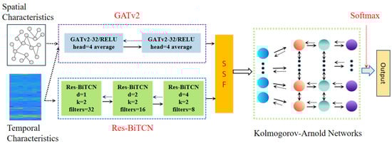
Figure 1.
The structure of the DST-TSA.
2.1. The Working Mechanism of Improved Graph Attention Network
GCN and GAT are two classical GNN architectures widely used for spatial feature extraction. The core idea of GCN is to update node representations (e.g., bus nodes, load nodes) by aggregating information transmitted through edges. Building upon this, GAT introduces an attention mechanism that adaptively evaluates the correlation between a node and its neighbors, allowing the model to assign higher weights to more influential nodes and lower weights to less relevant ones. This enables the extraction of richer topological information. In GAT, attention coefficients are computed in parallel for all neighboring nodes, ensuring flexible weighting during updates. However, its static attention mechanism restricts each node to attend to neighbors using itself as the sole query, which limits expressive power and may hinder performance on complex tasks. To overcome this drawback, this study adopts GATv2, which employs a dynamic attention mechanism by modifying the node update process, thereby enhancing the model’s ability to capture complex spatial dependencies.
In GATv2, the input to any single layer is a set of node feature vectors, defined as
where to the -th layer of the GATv2, and denotes the number of nodes in the power system.
The output of the graph attention layer is a set of updated feature vectors for each node in the power system, defined as
where represents the output of the -th layer; and have different dimensions.
The dynamic attention coefficient calculation in GATv2 is as follows:
where represents the learnable weight matrix; represents the learnable weight vector; denotes the matrix concatenation operation; and is the activation function.
After applying the SoftMax activation function for normalization, the new attention coefficient is obtained, represented as
where denotes that r is the neighboring node of node .
After obtaining the normalized attention coefficient , feature aggregation is performed on node at the -th layer, resulting in the output of the -th layer, represented as
where represents the activation function, which usually chooses the ELU function. Its expression is as follows:
This activation function combines the properties of sigmoid and ReLU, featuring soft saturation on the left and linearity on the right. The linear region allows ELU to alleviate the gradient vanishing issue inherent in the sigmoid, while the soft saturation region introduces sparsity similar to ReLU. Moreover, this design facilitates faster convergence during training. The value of parameter is typically set to 1.
The single attention mechanism may be insufficient for producing stable and diverse representations. To improve learning capacity and stability, -independent attention mechanisms are employed to compute attention coefficients, and their outputs are concatenated as follows:
where represents the attention coefficients obtained by the -th attention mechanism and denotes the learnable weight matrix of the -th attention mechanism.
The features are averaged as
The working process of the improved GAT with K attention mechanisms is shown in Figure 2.
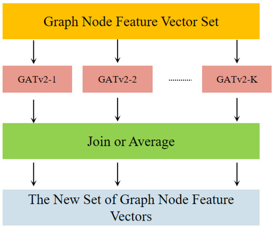
Figure 2.
The working process of the GAT.
2.2. The Working Mechanism of Residual Bidirectional Temporal Convolutional Network
Temporal convolutional network (TCN) [28] is an extension of CNN designed for time-series modeling, with its core mechanisms being causal convolution and dilated convolution. When applied to transient stability data in power systems, TCN employs causal dilated convolution to capture temporal dependencies. The formulation of causal dilated convolution is given as
where represents the output at time ; is the -th filter; is the input data at time ; is the dilation coefficient; and is the size of the convolution kernel.
BiTCN consists of two oppositely oriented TCN layers, as shown in Figure 3, and offers two main advantages: the bidirectional modeling and mitigation of gradient vanishing. By incorporating TCN layers in both temporal directions, BiTCN simultaneously leverages past and future voltage information, thereby capturing time-series characteristics more effectively than standard TCN and achieving improved stability and reliability.
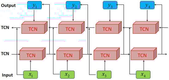
Figure 3.
The architecture of BiTCN.
In deep learning, increasing network depth often introduces training difficulties due to vanishing or exploding gradients. Residual networks address these challenges by introducing shortcut connections, which enhance information flow, suppress gradient issues, reduce parameter complexity, and accelerate convergence. Motivated by these benefits, this study integrates residual connections into the feature-fusion BiTCN by adding an identity mapping path, thereby constructing the Res-BiTCN model. The computation process of Res-BiTCN is formulated as follows:
where denotes the network input, and represents the extracted feature output.
2.3. The Spatio-Temporal Feature Fusion Layer
To comprehensively extract both the bidirectional temporal features and spatial features of transient data, a spatio-temporal feature fusion layer is constructed on top of the GATv2 and Res-BiTCN layers. Specifically, the output of the GATv2 layer is a two-dimensional tensor containing the spatial feature representations of the system, while the output of the Res-BiTCN layer is a three-dimensional tensor containing bidirectional temporal feature representations. Due to their dimensional mismatch, both outputs are reshaped into one-dimensional tensors and concatenated along the feature dimension, thereby forming a unified representation of transient spatio-temporal features. This fusion strategy provides a more comprehensive characterization of transient information, which in turn enhances the accuracy and reliability of TSA.
2.4. The Working Mechanism of Kolmogorov–Arnold Network
Multilayer perceptrons (MLPs), or fully connected feedforward networks, are fundamental components in deep learning and are widely used to approximate nonlinear functions. However, their fully connected structure requires configuring a large number of parameters, many of which contribute little to model efficiency.
The design of the KAN is inspired by the Kolmogorov–Arnold representation theorem, which states that any multivariable continuous function can be expressed as a composition of univariate functions. Unlike MLPs with fixed activation functions, KAN incorporates learnable activation functions directly into the connection weights. These functions, often parameterized by B-splines, enable flexible nonlinear mappings from inputs to outputs without relying solely on weighted summation. The underlying principles are as follows:
For an -dimensional continuous function , it can be expressed as
where ; ; represents the number of neurons in the hidden layer.
Let the control points be and the nodes be , then an -th order B-spline function can be constructed using the recursive formula:
where ; . Thus, the equation of the B-spline is
In the KAN model, the activation function is mathematically expressed as
where , and both parameters and are initialized by using the Xavier method.
For a KAN model with depth , its architecture can be represented by an integer array. Let denote the activation function connecting the -th layer to the -th layer, where , , and . The output of the -th layer can be expressed as
where represents the input to the -th layer.
Therefore, KAN with depth can be expressed as
3. TSA Model Based on DST-TSA
As a data-driven method, the core of implementing TSA with the DST-TSA method is to construct a high-performance classifier capable of accurately learning the implicit mapping between electrical measurements and transient stability states through offline training. Once trained, the model can be deployed on the WAMS master station for online application, enabling the real-time assessment of grid transient stability. This section details several key aspects of the implementation process.
3.1. The Input and Output of the Model
Input feature selection is a key factor in determining model performance, as it directly affects the extraction of comprehensive and discriminative information from high-dimensional measurement data. To fully capture the spatio-temporal characteristics of power system transients, the model input is organized along both spatial and temporal dimensions. For spatial features, the system topology is represented by an adjacency matrix. This accounts for the influence of grid structure on energy distribution and transfer pathways, while also reflecting dynamic interactions among nodes to capture the spatial evolution of transient data. For temporal features, transient stability is influenced by multiple variables. Voltage magnitude and phase angle reflect the system’s dynamic response and are closely tied to stability conditions, whereas active and reactive power describe power flow and consumption patterns within the system. The variations in these quantities can induce voltage fluctuations and increase the risk of transient instability. Therefore, this study selects the voltage magnitude (), phase angle (), active power (), and reactive power () at each system node across the pre-fault, fault-on, and post-fault stages as input features, formulated as
where denotes the number of sampling points; represents the number of nodes; and , , , and indicate the voltage magnitude, phase angle, active power injection, and reactive power injection, respectively, at node at time instant .
3.2. The Output of Evaluation Model and Stability Criterion
The output of the evaluation model is a binary stability label, where denotes a stable system and denotes an unstable system. The transient stability of each sample is determined using the transient stability index (TSI), defined based on the post-disturbance rotor angle as
where represents the maximum relative rotor angle difference between any two generators during the simulation period. When , the sample is identified as stable; otherwise, it is considered unstable.
3.3. The Weighted Cross-Entropy Loss Function for Imbalanced Samples
In practical scenarios of transient stability analysis in power systems, the distribution of stable and unstable samples is inherently imbalanced. Specifically, most operating conditions correspond to stability, whereas transient instability cases are relatively rare. However, in real-world applications, the accurate assessment of unstable cases is of greater concern. Inspired by edge detection techniques in the field of image recognition, this study adopts a weighted cross-entropy function as the loss function during training, formulated as follows:
where denotes the number of training samples per iteration; and are Boolean labels indicating whether sample k belongs to unstable or stable classes; and represent the model’s output probability values; is the weight assigned to unstable samples; and is the weight assigned to stable samples. In this study, the weights and are determined according to the ratio of unstable to stable samples, defined as
where and denote the numbers of stable and unstable samples, respectively. This setting ensures that the minority unstable class receives a larger penalty, thereby alleviating the imbalance problem and improving the reliability of instability prediction.
3.4. Evaluation Metrics
To comprehensively assess the training and testing performance, the TSA confusion matrix shown in Table 1 is adopted.

Table 1.
Confusion matrix for TSA.
This paper employs accuracy (), precision (), recall (), and F-score () as evaluation metrics, defined as follows:
where directly reflects the model’s overall correctness in judging system stability status; indicates the model’s judgment accuracy for unstable states; represents the model’s detection capability for unstable states; and comprehensively considers both precision and recall, balancing the model’s accuracy and completeness in identifying unstable conditions.
4. Case Study Analysis
4.1. The New England 10-Machine 39-Bus System
4.1.1. The Construction of Sample Set
The dataset is derived from fault simulation conducted on the New England 10-machine 39-bus system [29] using Power System Toolbox (PST) version 3.0, which provides high-fidelity power system simulation data, establishing a solid foundation for model training and testing. The system configuration is illustrated in Figure 4, while the details of sample set construction are presented in Table 2. The samples are preprocessed using the min–max normalization method to scale the input features of the TSA model into the range of [0, 1]. Subsequently, the dataset is partitioned into training and testing subsets at a ratio of 5:1, ensuring a rigorous and balanced evaluation of model performance.
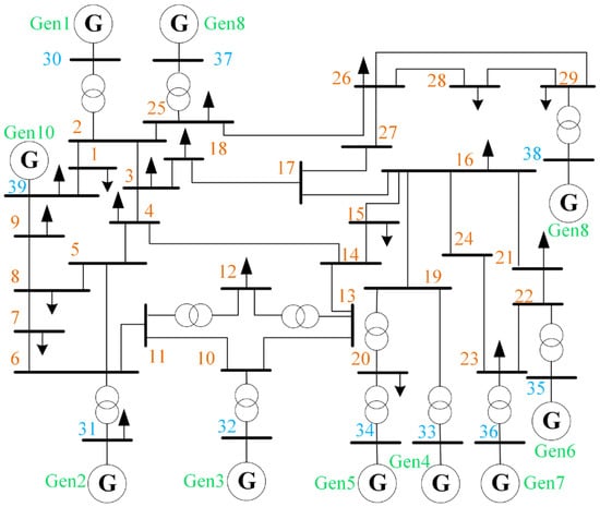
Figure 4.
The structural diagram of the New England 10-machine 39-bus system.
Table 2.
Details of sample set construction.
4.1.2. The Comparative Analysis of Model Performance
To demonstrate the superiority of the proposed DST-TSA method, this paper conducts comparative validation against several widely used machine learning methods, including RF, SVM, and four deep learning algorithms: GCN, TCN, LSTM, and CNN. All aforementioned deep learning models are trained and optimized using the Adam optimizer. Compared to conventional stochastic gradient descent (SGD), the Adam algorithm incorporates momentum and exponentially weighted moving averages, which effectively suppresses gradient oscillations and accelerates model convergence. The remaining hyperparameters of the model are configured as follows: the learning rate is set to 0.001, with a batch size of 100 and 100 training epochs. The dropout rate is set to 0.4, and the sampling window length is fixed at 25. In addition, the classification threshold is set to 0.5; if the predicted value of a node is greater than or equal to 0.5, the system is considered unstable, whereas values below 0.5 indicate a stable system. The predictive performance of the proposed DST-TSA model and the six baseline models on the test set is presented in Table 3 and Figure 5.
Table 3.
Test results of seven models.
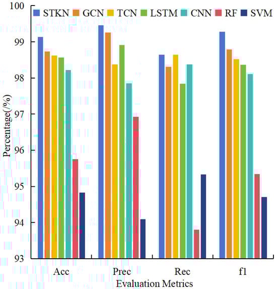
Figure 5.
The comparative evaluation results of seven models.
As evidenced by the test metrics presented in Table 3 and Figure 5, the proposed model demonstrates significant advantages over SVM, RF, CNN, and LSTM models across all evaluation criteria-accuracy, precision, recall, and -score. Among these models, CNN and LSTM show superior prediction performance over SVM and RF by effectively learning temporal characteristics from input data. However, they fail to fully exploit the spatio-temporal features inherent in transient stability data, resulting in lower prediction performance compared to the proposed DST-TSA method. Although GCN and TCN exhibit relatively competitive performance by capturing either spatial or temporal dependencies, their inability to jointly model spatio-temporal correlations still limits their effectiveness compared with the proposed approach.
4.1.3. The Ablation Experiment
To demonstrate the effectiveness of individual components in the DST-TSA method, two incomplete DST-TSA methods are constructed for ablation study.
In practical online applications: The Res-BiTCN module is removed, preserving only GATv2 and KAN to capture spatial distribution characteristics in post-fault transient stability data.
Ablation Model 2: The GATv2 module is removed, preserving only Res-BiTCN and KAN to extract temporal correlation in post-fault transient stability data.
The ablation study results in Table 4 demonstrate that removing either the Res-BiTCN or GATv2 module results in degraded performance. Specifically, Ablation Model 1, which removes the Res-BiTCN while retaining GATv2 and KAN, exhibits reductions across all evaluation metrics compared with the complete DST-TSA method. This confirms the critical role of Res-BiTCN in capturing bidirectional temporal features from transient data, effectively extracting the dynamic evolution patterns of post-fault voltages to provide more precise temporal information for TSA. Similarly, Ablation Model 2, which removes GATv2 while preserving Res-BiTCN and KAN, also shows performance degradation. This underscores the indispensable role of GATv2 in extracting spatial distribution patterns, as it leverages system topology to reveal spatial correlations among nodes and thereby supplies essential spatial feature information for TSA. Overall, Res-BiTCN and GATv2 serve complementary functions within DST-TSA, jointly enhancing spatio-temporal feature extraction and ultimately improving overall assessment performance.
Table 4.
Results of ablation experiment.
4.1.4. Performance Comparison Among GATv2, Res-BiTCN and GAT, BiTCN
To validate the performance advantages of GATv2 and Res-BiTCN over their baseline models, namely GAT and BiTCN, comparative experiments are conducted. The experimental results are presented in Figure 6.
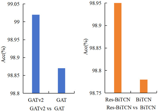
Figure 6.
Performance comparison among four models: GATv2, Res-BiTCN, and GAT, BiTCN.
The test results indicate that GATv2 achieves superior prediction accuracy compared with GAT, particularly in handling complex power grid graph structures. In addition, the incorporation of a residual network structure enables Res-BiTCN to effectively extract both forward and backward temporal features while alleviating network degradation, thereby enhancing performance in TSA tasks.
4.1.5. Performance Analysis Under Noisy Conditions
In practical online applications, the test dataset originates from real-time PMU data. However, due to potential measurement inaccuracies in PMU readings of dynamic data, errors may be introduced. To simulate such measurement noise in real applications, Gaussian white noise is incorporated into the test dataset. The instantaneous values of this noise follow a Gaussian distribution, while its power spectral density exhibits a uniform distribution. The specific methodology for constructing the noise is as follows:
where represents the noise-free test set; denotes the test set after Gaussian white noise injection; and follows a Gaussian distribution with 0 mean and variance .
The pre-trained model is tested using the Gaussian white noise-contaminated test set , with the evaluation results exhibited in Figure 6.
As evidenced by Figure 7, in shallow machine learning algorithms, RF and SVM exhibit rapid accuracy degradation and significant performance fluctuations with increasing noise levels, demonstrating their limited robustness. In contrast, the proposed method in this paper maintains superior prediction accuracy compared to both LSTM and CNN models under noisy conditions, confirming its better robustness.
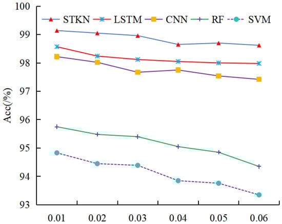
Figure 7.
Model performance comparison under noisy conditions.
4.1.6. Generalization Performance Evaluation Under Unseen Scenarios
To emulate unforeseen operating condition variations that dispatchers may encounter in online applications and to further evaluate the generalization capability of the proposed DST-TSA method, the system load level was increased to 125% of the base load, and three transmission lines were randomly removed. Correspondingly, generator outputs were adjusted to ensure convergence of the power flow calculation. The fault configurations, including faulted lines, fault locations, clearing times, and fault types, remained identical to those in Section 4.1.1. Under these conditions, a total of 3500 simulation samples were generated, comprising 1952 unstable cases and 1548 stable cases. The model, trained offline in Section 4.1.2, was directly applied, and the testing results in this overloaded scenario are summarized in Figure 8.
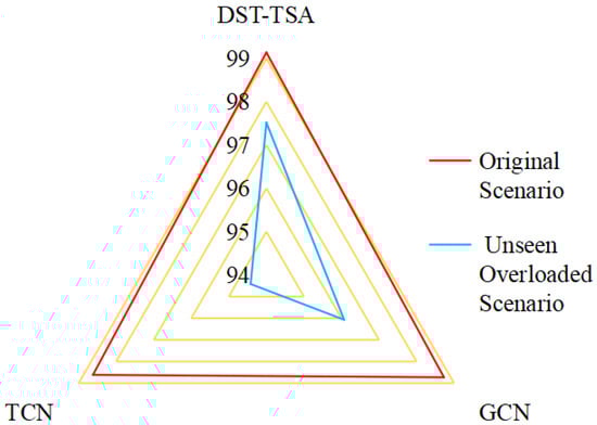
Figure 8.
Generalization accuracy of each model with unseen scenarios.
Under significantly varying operating conditions, the proposed DST-TSA method still maintains high testing accuracy, achieving 97.52%, which outperforms the other two comparative approaches. Among them, GAT also demonstrates competitive performance, with an accuracy only 1.45% lower than that of DST-TSA. This result indicates that both GAT and DST-TSA are capable of effectively capturing the spatial features of transient data. Consequently, when the system topology and load levels change, their input adjacency matrices can promptly reflect these variations, thereby preventing significant degradation in model performance. In contrast, the TCN model, which fails to exploit spatial feature information of power systems, exhibits a noticeable decline in prediction accuracy under such scenarios.
4.2. Large-Scale Power Grid Testing
To further validate the effectiveness of the proposed DST-TSA method, a large-scale NPCC 48-machine 140-bus system was employed for testing. This system consists of 48 generators, 140 buses, and 233 transmission lines. During sample simulations, the load level ranged from 90% to 110% of the base load, in 5% increments. A three-phase short-circuit fault was adopted as the contingency type, and four different fault clearing times were considered, corresponding to the 7th, 10th, 13th, and 16th cycles after fault occurrence. Based on these settings, a total of 12,675 samples were generated, including 6790 stable cases and 5885 unstable cases. The dataset was randomly divided into training and testing subsets with a ratio of 6:1.
As shown in Table 5, the proposed DST-TSA method consistently outperforms GCN and TCN even on the larger-scale power system. This demonstrates that DST-TSA is more suitable for practical applications in ultra-large power grids, thereby providing more reliable support for operational scheduling and state estimation.
Table 5.
Results of metrics for three models.
5. Conclusions
Power system transient data inherently exhibit spatio-temporal distribution characteristics. To effectively exploit these properties, this study proposes a deep spatio-temporal feature-extraction approach for TSA. The proposed approach is validated using the New England 10-machine 39-bus system and the NPCC 48-machine 140-bus system. The key findings are summarized as follows.
(1) Compared with other methods, the proposed framework exhibits superior capability in comprehensively extracting spatio-temporal features from grid data, effectively capturing the evolutionary patterns of transient behavior and thereby ensuring high assessment accuracy.
(2) With the integration of a dynamic attention mechanism, GATv2 achieves enhanced representational capacity, enabling the more effective processing of complex grid structures. In parallel, the incorporation of residual connections into the BiTCN yields the Res-BiTCN architecture, which not only captures both forward and backward temporal features but also alleviates the network degradation problem.
(3) The proposed method maintains high prediction accuracy under noisy PMU measurement data, demonstrating superior robustness.
Future research will focus on unsupervised and semi-supervised learning to leverage the large volumes of unlabeled power system data, thereby further exploiting their potential value and enabling a more refined TSA of transient rotor angle stability.
Author Contributions
Conceptualization, Y.N. and M.T.; methodology, Y.N.; software, Y.Z. and H.Z.; validation, Y.N. and Z.K.; formal analysis, M.T. and Y.Z.; investigation, H.Z.; resources, H.Z.; data curation.; writing—original draft preparation, Y.N.; writing—review and editing, H.Z.; visualization, H.Z. and Y.Z.; supervision, Z.K.; project administration, Z.K. All authors have read and agreed to the published version of the manuscript.
Funding
This research received no external funding.
Data Availability Statement
The original data presented in the study are openly available on GitHub at https://github.com/yangyuan123654/yydata (accessed on 25 August 2025).
Conflicts of Interest
Authors Yu Nan, Meng Tong, and Zhenzhen Kong were employed by the company State Grid Henan Electric Power Company Kaifeng Power Supply Company. The remaining authors declare that the research was conducted in the absence of any commercial or financial relationships that could be construed as a potential conflict of interest.
References
- Xia, S.; Zhang, C.; Li, Y.; Li, G.; Ma, L.; Zhou, N. GCN-LSTM Based Transient Angle Stability Assessment Method for Future Power Systems Considering Spatial-Temporal Disturbance Response Characteristics. Prot. Control Mod. Power Syst. 2024, 9, 108–121. [Google Scholar] [CrossRef]
- Liu, C.; Li, B.; Zhang, Y.; Jiang, Q.; Liu, T. The LCC Type DC Grids Forming Method and Fault Ride-Through Strategy Based on Fault Current Limiters. Int. J. Electr. Power Energy Syst. 2025, 170, 110843. [Google Scholar] [CrossRef]
- Wu, S.; Zheng, L.; Hu, W.; Yu, R.; Liu, B. Improved Deep Belief Network and Model Interpretation Method for Power System Transient Stability Assessment. J. Mod. Power Syst. Clean Energy 2020, 8, 27–37. [Google Scholar] [CrossRef]
- Zadkhast, P.; Jatskevich, J.; Vaahedi, E. A Multi-Decomposition Approach for Accelerated Time-Domain Simulation of Transient Stability Problems. IEEE Trans. Power Syst. 2015, 30, 2301–2311. [Google Scholar] [CrossRef]
- Vu, T.L.; Turitsyn, K. Lyapunov Functions Family Approach to Transient Stability Assessment. IEEE Trans. Power Syst. 2016, 31, 1269–1277. [Google Scholar] [CrossRef]
- Diao, R.; Vittal, V.; Logic, N. Design of a Real-Time Security Assessment Tool for Situational Awareness Enhancement in Modern Power Systems. IEEE Trans. Power Syst. 2010, 25, 957–965. [Google Scholar] [CrossRef]
- Sun, K.; Likhate, S.; Vittal, V.; Kolluri, V.S.; Mandal, S. An Online Dynamic Security Assessment Scheme Using Phasor Measurements and Decision Trees. IEEE Trans. Power Syst. 2007, 22, 1935–1943. [Google Scholar] [CrossRef]
- Gao, Q.; Rovnyak, S.M. Decision Trees Using Synchronized Phasor Measurements for Wide-Area Response-Based Control. IEEE Trans. Power Syst. 2011, 26, 855–861. [Google Scholar] [CrossRef]
- Dong, L.; Du, H.; Mao, F.; Han, N.; Li, X.; Zhou, G. Very High Resolution Remote Sensing Imagery Classification Using a Fusion of Random Forest and Deep Learning Technique—Subtropical Area for Example. IEEE J. Sel. Topics Appl. Earth Observ. Remote Sens. 2020, 13, 113–128. [Google Scholar] [CrossRef]
- Sotnikov, D.; Lyly, M.; Salmi, T. Prediction of 2G HTS Tape Quench Behavior by Random Forest Model Trained on 2-D FEM Simulations. IEEE Trans. Appl. Supercond. 2023, 33, 6602005. [Google Scholar] [CrossRef]
- Geeganage, J.; Annakkage, U.D.; Weekes, T.; Archer, B.A. Application of Energy-Based Power System Features for Dynamic Security Assessment. IEEE Trans. Power Syst. 2015, 30, 1957–1965. [Google Scholar] [CrossRef]
- Ertekin, S.; Bottou, L.; Giles, C.L. Nonconvex Online Support Vector Machines. IEEE Trans. Pattern Anal. Mach. Intell. 2011, 33, 368–381. [Google Scholar] [CrossRef] [PubMed]
- He, M.; Vittal, V.; Zhang, J. Online Dynamic Security Assessment with Missing PMU Measurements: A Data Mining Approach. IEEE Trans. Power Syst. 2013, 28, 1969–1977. [Google Scholar] [CrossRef]
- Ma, R.; Eftekharnejad, S.; Zhong, C. Predictive Online Transient Stability Assessment for Enhancing Efficiency. IEEE Open Access J. Power Energy 2024, 11, 207–217. [Google Scholar] [CrossRef]
- Liu, W.; Kerekes, T.; Dragicevic, T.; Teodorescu, R. Review of Grid Stability Assessment Based on AI and a New Concept of Converter-Dominated Power System State of Stability Assessment. IEEE J. Emerg. Sel. Topics Ind. Electron. 2023, 4, 928–938. [Google Scholar] [CrossRef]
- Shen, Y.; Wang, Y.; Li, Y.; Wang, Z.; Huang, C.; Blaabjerg, F. Hierarchical Time-Series Assessment and Control for Transient Stability Enhancement in Islanded Microgrids. IEEE Trans. Smart Grid 2023, 14, 3362–3374. [Google Scholar] [CrossRef]
- Badran, Y.; Isbeih, Y.J.; Moursi, M.S.E.; Al Hosani, K.H. A Data Driven Stability Assessment Approach for Multiple Microgrids Interconnection. IEEE Trans. Ind. Appl. 2025, 61, 2646–2661. [Google Scholar] [CrossRef]
- Yan, R.; Geng, G.; Jiang, Q.; Li, Y. Fast Transient Stability Batch Assessment Using Cascaded Convolutional Neural Networks. IEEE Trans. Power Syst. 2019, 34, 2802–2813. [Google Scholar] [CrossRef]
- Shi, Z.; Yao, W.; Zeng, L.; Wen, J.; Fang, J.; Ai, X.; Wen, J. Convolutional Neural Network-Based Power System Transient Stability Assessment and Instability Mode Prediction. Appl. Energy 2020, 263, 114856. [Google Scholar] [CrossRef]
- Yu, J.J.Q.; Hill, D.J.; Lam, A.Y.S.; Gu, J.; Li, V.O.K. Intelligent Time-Adaptive Transient Stability Assessment System. IEEE Trans. Power Syst. 2018, 33, 1049–1058. [Google Scholar] [CrossRef]
- Shao, Z.; Wang, Q.; Cao, Y.; Cai, D.; You, Y.; Lu, R. A Novel Data-Driven LSTM-SAF Model for Power Systems Transient Stability Assessment. IEEE Trans. Ind. Informat. 2024, 20, 9083–9097. [Google Scholar] [CrossRef]
- Li, B.; Wu, J. Adaptive Assessment of Power System Transient Stability Based on Active Transfer Learning with Deep Belief Network. IEEE Trans. Autom. Sci. Eng. 2023, 20, 1047–1058. [Google Scholar] [CrossRef]
- Tan, B.; Yang, J.; Tang, Y.; Jiang, S.; Xie, P.; Yuan, W. A Deep Imbalanced Learning Framework for Transient Stability Assessment of Power System. IEEE Access 2019, 7, 81759–81769. [Google Scholar] [CrossRef]
- Umbereen, S.; Weiss, X.; Rolander, A.; Ghandhari, M.; Eriksson, R. Investigating the Performance of MLE and CNN for Transient Stability Assessment in Power Systems. IEEE Access 2024, 12, 125095–125107. [Google Scholar] [CrossRef]
- Lee, G.; Park, C.; Kim, D.-I. Event Detection-Free Framework for Transient Stability Prediction via Parallel CNN-LSTMs. IEEE Trans. Instrum. Meas. 2024, 73, 9004410. [Google Scholar] [CrossRef]
- Huang, J.; Guan, L.; Su, Y.; Yao, H.; Guo, M.; Zhong, Z. A Topology Adaptive High-Speed Transient Stability Assessment Scheme Based on Multi-Graph Attention Network with Residual Structure. Int. J. Electr. Power Energy Syst. 2021, 130, 106948. [Google Scholar] [CrossRef]
- Shao, C.; He, X.; Ma, L.; Wang, H.; Zhou, C.; Dong, H. Transient Assessment of Power Systems Based on Graph Attention Networks. In Proceedings of the 2024 IEEE 5th International Conference on Advanced Electrical and Energy Systems (AEES), Lanzhou, China, 29 November–1 December 2024; pp. 525–530. [Google Scholar]
- Massaoudi, M.; Zamzam, T.; Eddin, M.E.; Ghrayeb, A.; Abu-Rub, H.; Refaat, S.S. Fast Transient Stability Assessment of Power Systems Using Optimized Temporal Convolutional Networks. IEEE Open J. Ind. Appl. 2024, 5, 267–282. [Google Scholar] [CrossRef]
- Taj, T.A.; Hasanien, H.M.; Alolah, A.I.; Muyeen, S.M. Transient Stability Enhancement of a Grid-Connected Wind Farm Using an Adaptive Neuro-Fuzzy Controlled-Flywheel Energy Storage System. IET Renew. Power Gener. 2015, 9, 792–800. [Google Scholar] [CrossRef]
Disclaimer/Publisher’s Note: The statements, opinions and data contained in all publications are solely those of the individual author(s) and contributor(s) and not of MDPI and/or the editor(s). MDPI and/or the editor(s) disclaim responsibility for any injury to people or property resulting from any ideas, methods, instructions or products referred to in the content. |
© 2025 by the authors. Licensee MDPI, Basel, Switzerland. This article is an open access article distributed under the terms and conditions of the Creative Commons Attribution (CC BY) license (https://creativecommons.org/licenses/by/4.0/).