Identification of Key Parameters and Construction of Empirical Formulas for Isentropic and Volumetric Efficiency of High-Temperature Heat Pumps Based on XGBoost-MLR Algorithm

Abstract

High-temperature heat pumps (HTHPs) have gradually begun to play an essential role in using heat in industry for waste heat recovery and providing higher-grade heat. The isentropic efficiency and volumetric efficiency of HTHPs are significantly affected by high-temperature operating conditions, which take the pressure ratio (PR) as the key parameter, with limited consideration of other factors such as temperature. Relying on the experimental data obtained from the industrial-grade HTHP system experimental platform, this work proposed an XGBoost-MLR algorithm-based method to identify the key parameters of HTHP isentropic efficiency and volumetric efficiency. High-precision (R² > 0.95) prediction models were established to determine the effect of temperature variables on isentropic efficiency and volumetric efficiency. After the key parameters were identified, the empirical equation of isentropic efficiency and volumetric efficiency applicable to this operation condition were constructed. The average relative errors of the two empirical formulas were 5.95% and 5.28%, respectively. Finally, the generalizability of empirical formulas was verified using experimental data from other researchers. The isentropic empirical formula had a relative deviation of less than 10% under twin-screw compressor conditions. However, the applicability of the volumetric efficiency empirical formula was unstable in compressors of different sizes. The feasibility of the method was also discussed.

1. Introduction

“Energy-saving and low carbon” is a research hotspot for governments and researchers worldwide. However, the world still faces a significant problem of energy waste and high carbon emissions, evident in the industrial sector. In 2022, China’s industrial energy consumption accounted for more than 65% of total energy consumption, of which thermal energy consumption accounted for more than 50% [1]. The irrational utilization of industrial waste heat, coupled with the prevalent use of inefficient and high-carbon-emitting heating equipment such as coal-fired and gas boilers, has significantly contributed to the squandering of industrial heat and the surge in carbon emissions. Heat pumps are a good option for industrial waste heat recovery, as they can use low-grade industrial waste heat as a heat source to prepare high-grade heat for other heat demand scenarios with high efficiency. The development of high-temperature heat pumps (HTHPs) provides an alternative to traditional heating equipment such as coal-fired boilers [2]. Figure 1 shows the heat demand temperature of different industries in the industrial field [3]. In most industries where the demand temperature is less than 200 °C, HTHPs can satisfy heating temperature requirements and significantly improve energy efficiency and reduce CO₂ emissions.

Vapor compression HTHPs are widely used in industry (this is also the type of heat pump introduced in this work, indicated by the abbreviation HTHPs). The compressor is one of the most critical components of an HTHP and has a significant impact on performance-related parameters such as heating capacity and coefficient of performance (COP). It also affects economic parameters such as system life [4]. To ensure the stable and efficient operation of HTHPs, it is essential to choose the appropriate compressor based on factors such as working temperature ranges, refrigerant injection quantity, and other considerations. Currently, the compressors used in industrial-grade HTHPs are mainly screw compressors (including single- and twin-screw compressors) and piston compressors [2,5,6,7,8,9,10]. Twin-screw compressors offer better isentropic efficiency, volumetric efficiency, and energy savings. In recent years, with the development of HTHP units, especially in large units with high heat production temperatures and high heat demand, the use of twin-screw compressors has gradually increased. Examples include the SGH120 and SGH165 series developed by Kobe Steel, which use high-temperature-resistant twin-screw compressors [5] to prepare steam at 120 °C/165 °C.

Compressor isentropic efficiency is a parameter that reacts to the irreversible losses of the compressor and is one of the critical parameters that respond to the performance of the HTHPs. During the operation of the compressor, the irreversible losses mainly come from processes such as heat dissipation, leakage, and friction. When conducting an analysis of the HTHP system, researchers found that the temperature parameter of the compressor under high-temperature operating conditions had a significant effect on the isentropic efficiency. Wang et al. [11] found experimentally that the cooling oil temperature substantially impacts the isentropic efficiency of twin-screw compressors. Lowering the oil temperature under certain conditions can improve compressor performance. Zhao et al. [12] developed a semi-empirical model for twin-screw compressors based on experimental data. The temperature parameters of the model were optimized. The study found that reducing the operating temperature of the compressor can increase the isentropic efficiency by more than 10%. Afshari et al. [13] showed experimentally that the isentropic efficiency of reciprocating compressors was significantly affected by the lubricant viscosity, which was correlated with the operating temperature of the compressor. In addition, some researchers have demonstrated during experiments and simulations that the isentropic efficiency of compressors in HTHP systems is significantly affected by the operating temperature [14,15,16]. However, in HTHP simulation and performance evaluation, the influence of temperature on isentropic efficiency was still not taken seriously. The commonly used empirical formula for isentropic efficiency (shown in

Table 1. Research table for empirical formula of isentropic efficiency.

Researcher	Compressor Types	Refrigerants	The Empirical Formula for Isentropic Efficiency	Condensing Temperature/°C	Conformity of Data for This Work (R2)
Sulaiman [17]	Piston compressors	R245fa, R1233Zzd(E)	${\eta }_{\mathrm{s}}=a_1+a_2\cdot PR$	80~120	0.2136
Zhang [18]	Piston compressors	R245fa/R152a	${\eta }_{\mathrm{s}}=a_1+a_2\cdot P_{\mathrm{cond}}+a_3\cdot PR$	70~90	0.2803
Wang [19]	Twin-Screw Compressors	R744	${\eta }_s=a_1+a_2\cdot PR+a_3\cdot P{R}^2$	70~90	0.2766
Marwan [20]	Twin-Screw Compressors	R718	${\eta }_s=a_1+a_2\cdot PR+a_3\cdot Q$	100~130	0.3079
Wang [21]	Scroll compressors	R245fa	${\eta }_s=a_1+(1-{\mathrm{e}}^{{\displaystyle \frac{\mathrm{PR}+a_2}{a_3}}})-a_4\cdot \ln (PR+1)$	80~100	0

below) still took PR as the key parameter, with a lack of consideration for operating temperature. Meanwhile, Table 1 shows that the influencing factors of the isentropic efficiency vary according to different compressor types, refrigerants, and other factors. Therefore, it is necessary to discuss the key influencing factors of the isentropic efficiency, then establish a general identification method and reconstruct the empirical equation for isentropic efficiency based on the key parameters.

Volumetric efficiency is the ratio of the actual compressor discharge volume to the theoretical discharge volume. Volumetric efficiency reflects the refrigerant leakage of the compressor and is an important parameter that reflects the performance of the compressor. The volumetric efficiency empirical equations basically use the PR as the only variable in the different temperature zones of heat pumps [22,23,24]. The basic idea is to fit a polynomial using the PR. In addition, some researchers have also added variables such as compressor inlet pressure drop to further improve the accuracy of empirical equations [25]. Some researchers have also adapted to different scenarios by changing the form of empirical formulas [26]. In variable-speed compressors, researchers have used speed instead of the compression ratio for polynomial fitting [27], but the method has limitations. However, the empirical equations obtained from the PR fitting have a low fitting accuracy to the high-temperature heat pump operating data obtained in this work. The low fitting accuracy indicates that the existing empirical formulae for volumetric efficiency are no longer adequate to achieve accuracy in the operation of high-temperature heat pumps. This indicates the presence of other parameters affecting volumetric efficiency. For example, Zhao [12] found the effect of the temperature factor on volumetric efficiency in studying high-temperature heat pump compressors.

In recent years, machine learning algorithms have been used widely in the field of heat pumps. Many researchers have used machine learning algorithms to achieve breakthroughs in predicting heat pump energy consumption and optimizing control strategies. Machine learning algorithms provide a new way to investigate heat pumps, which can solve the original problem with a data-driven mindset. Ye et al. [28] used Artificial Neural Networks (ANNs) to perform energy consumption prediction of heat pump systems in remodeled houses. Relying on inputs of relevant variables such as time, outdoor temperature, and wind direction, the model ultimately achieved higher decision accuracy than traditional linear fitting methods. Miao et al. [29] constructed a fuzzy inference system based on machine learning algorithms for heat pump air conditioning. A prediction model of the passenger compartment and the set temperature was established to monitor and adaptively regulate the interior temperature. Noye et al. [30] explored the possibility of using machine learning to solve the multiparameter-influenced nonlinear dynamic optimization problem faced by ground-source heat pump systems. They believe that the system has great potential, both in building predictive models that reflect the actual performance and in optimizing control decisions in real time. Meanwhile, some researchers have made progress in thermal engineering using machine learning algorithms to identify key parameters. Yan et al. [31] used principal component analysis (PCA) and multiple linear regression algorithms (MLR) to identify key parameters in the organic Rankine cycle process. And an ANN prediction model was constructed, which had a relative error of less than 4%. Huang et al. [32] used the random forest algorithm (RF) included in the ensemble learning algorithm to identify key parameters in the building heating optimization process. A high-precision prediction model was built to determine the optimal set of variables. Ensemble learning algorithms can assess the importance of variables by observing splitting nodes in the process of building predictive models. However, the application of machine learning algorithms (e.g., ensemble learning algorithms) in identifying key influencing factors of heat pump performance still has not been reported.

Still, the accuracy of the ensemble learning algorithm’s importance assessment is significantly affected by the parameter interactions of the data set and the prediction accuracy of the model. The eXtreme Gradient Boosting (XGBoost) algorithm is one of the most advanced integration algorithms. It optimizes the input parameter interactions problem using regularization and column sampling to prevent overfitting. It also improves the model prediction accuracy by adopting the second Taylor series for the loss function. In addition, parallel optimization and sparse value optimization improve the algorithm’s efficiency. When a polynomial is used to fit the empirical equation for isentropic efficiency and volumetric efficiency, both are linearly related to the variables. The Multivariable Linear Regression (MLR) algorithm can respond well to the linear relationship between them, so it can be used to evaluate the contribution of parameters to isentropic efficiency and volumetric efficiency.

This work proposed a machine learning algorithm-based method for identifying the key parameters of isentropic and volumetric efficiency based on experimental data of industrial-grade HTHP steam engines. The XGBoost-MLR algorithm was applied to construct prediction models and identify key parameters. Orthogonal Transformation (OT), Grid search (GS), and Bayesian optimization (BO) algorithms were used to optimize the input parameter interaction problem and ensure model prediction accuracy. Based on the key parameters identified by the model, combined with the key variable of PR proposed by previous researchers, the empirical equations for isentropic efficiency and volumetric efficiency were finally reconstructed. The accuracy of both is demonstrated by comparing it with the isentropic efficiency obtained from experimental data. Finally, the generalizability of the empirical formula and the feasibility of the method is discussed. This work can provide some ideas and guidance for optimizing HTHP compressors in practical production.

2. Methodology

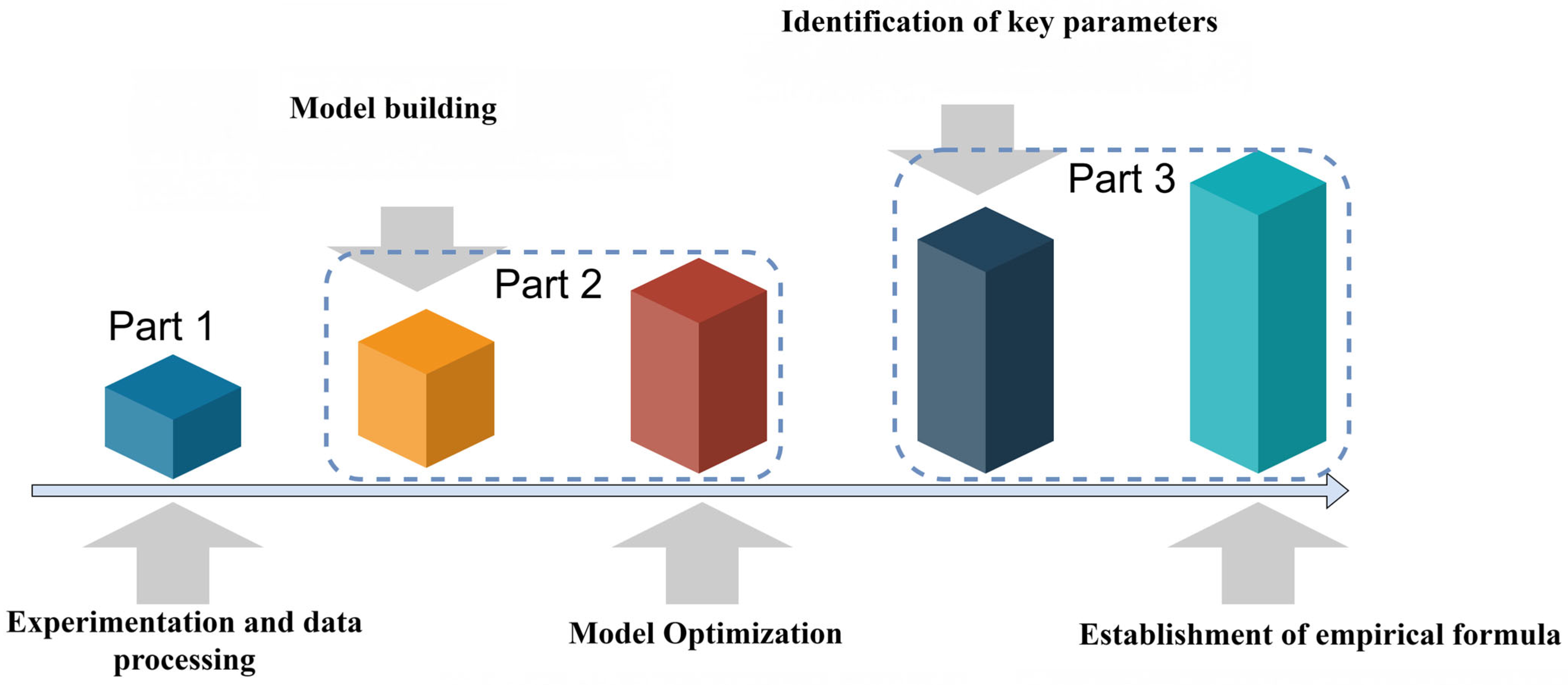
This work consists of three parts: (1) experiments and data acquisition, (2) model building and optimization, (3) model-based identification of key parameters and construction of empirical equations for isentropic and volumetric efficiency. The details are shown in Figure 2. In the experimental part, experiments were conducted with an industrial-grade HTHP system to obtain temperature-compliant data and select parameters related to isentropic and volumetric efficiency. The model building was carried out to establish a thermodynamic and prediction model based on a machine learning algorithm. Input parameters and hyperparameters were optimized by Orthogonal Transformation (OT), grid search (GS), and Bayesian optimization (BO) algorithms to improve model prediction accuracy and importance analysis. Hyperparameters are parameters whose values are set before starting the learning process. The key parameters of isentropic efficiency and volumetric efficiency were identified based on the optimization model. Then, the empirical equations were constructed. Finally, the generalizability of the empirical formulas and method was discussed.

2.1. Experiments and Data Processing

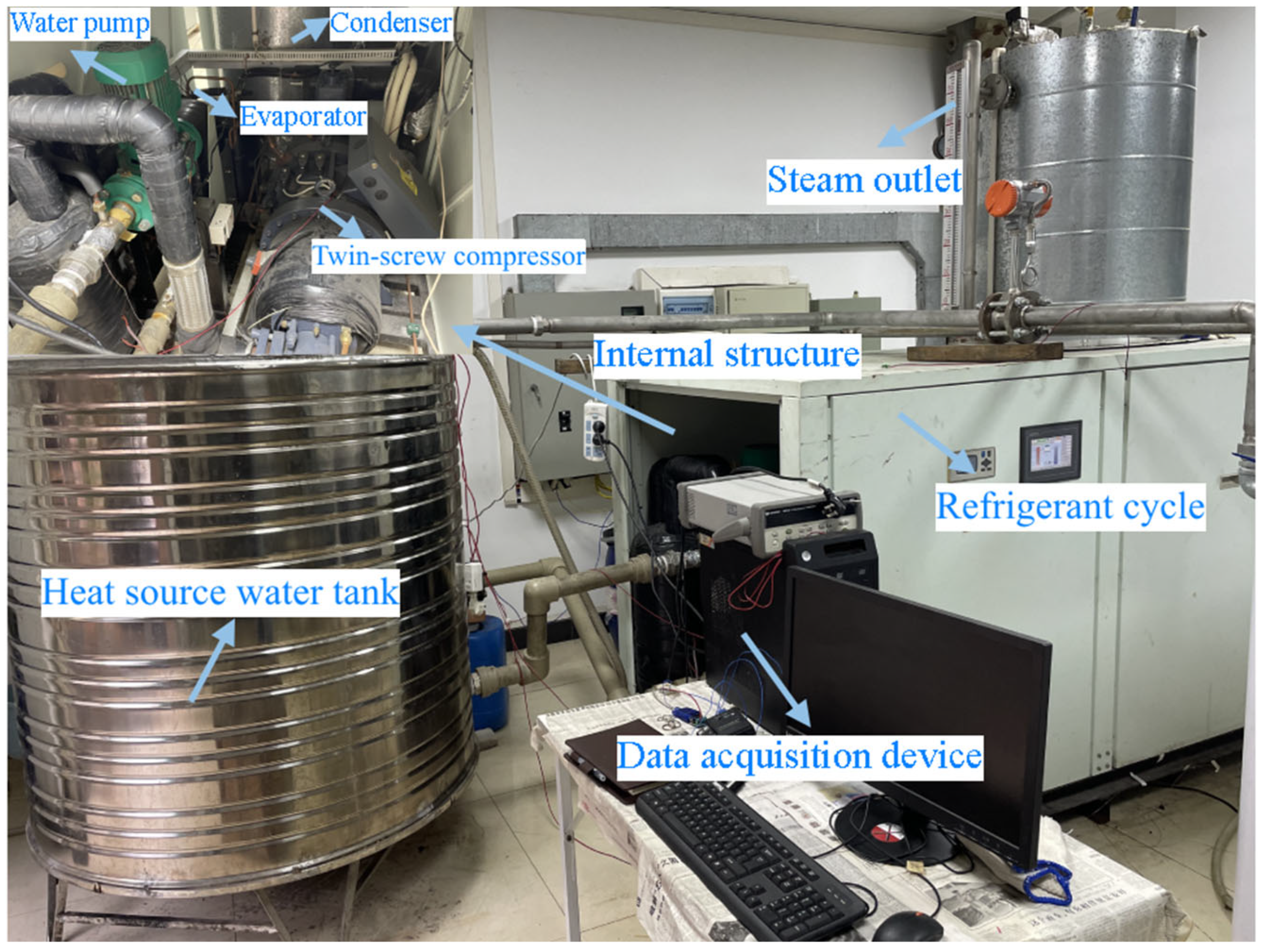
This work uses an 80 kW scale HTHP steam engine. Figure 3 shows the system equipment structure, including the refrigerant cycle, compressor oil cooling cycle, and heat source cycle. These location numbers represent temperature measurement points and pressure measurement points, which are measured by the platinum resistance temperature sensor of PT100 and diffused silicon pressure sensor of GPT220 produced in Shenzhen, China, respectively. Figure 4 shows an experimental site scenario using the HTHP unit.

2.1.1. Heat Source Cycle

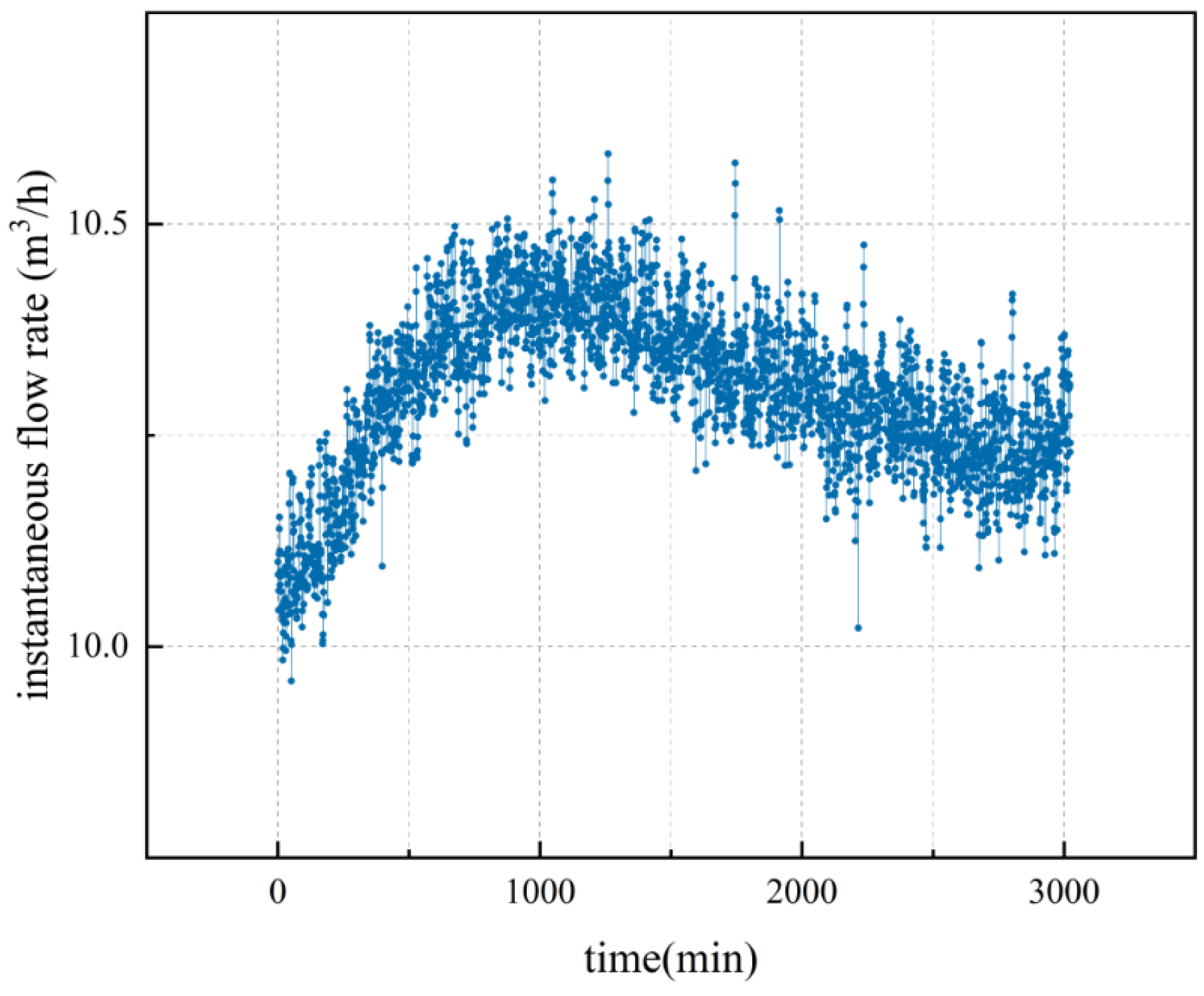
The cycle provides a stable heat source for the HTHP system. The principle of the process is shown in the heat source cycle section of Figure 3, which consists of a heat source tank, a water pump, and a heat exchanger. The heater maintains the heat source tank at the target temperature. The pump drives the heat source to exchange heat with the refrigerant in the heat exchanger continuously and steadily, during which the electromagnetic flow meter is used to detect the circulating water. In this experiment, the instantaneous flow rate was set to 10.25 m³/h. As shown in Figure 5, the fluctuation between the actual instantaneous flow rate and the assessed value does not exceed 3.3%, which is a steady state.

2.1.2. Refrigerant Cycle

The refrigerant cycle is the primary cycle of the heat pump system, mainly composed of a twin-screw compressor, electronic expansion valve, condenser, and evaporator. The refrigerant used in the cycle is R245fa. The cycle principle is shown in the refrigerant cycle section in Figure 3. The refrigerant exchanges heat with the heat source in the evaporator and is transformed into low-pressure superheated gas. Next, the gas is transformed into a high-temperature and high-pressure state through the compression of the compressor. Then, it enters the condenser and the subcooler for heat exchange and is transformed into a high-pressure liquid state. After being subjected to the throttling effect of the electronic expansion valve, it is transformed into a low-pressure gas–liquid mixture and enters the evaporator again, thus circulating.

2.1.3. Semi-Hermetic Twin-Screw Compressor Oil Cooling Cycle

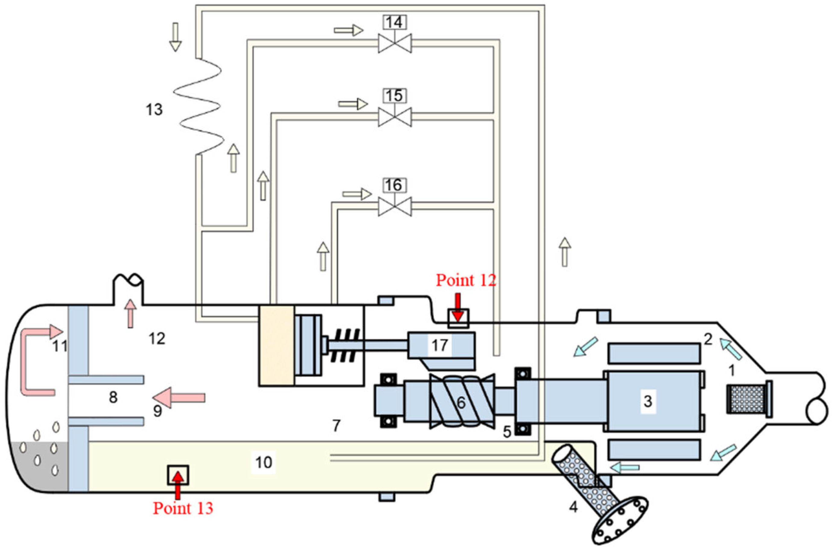
The screw compressor is cooled by an oil cooling system. The type of screw compressor used is the Hanbell RC2-200T series semi-hermetic twin-screw compressor produced in Shanghai, China. Figure 6 shows the structure of the compressor, which consists mainly of a capacity control slide valve, piston rod, piston cylinder, and piston ring. The details for the compressor component numbers are shown in

Table 2. Description of the oil cooling cycle of the twin-screw compressor.

Number	Component	Number	Component
1	Intake filter	10	Lubricating oil tank
2	Inlet gas (low-pressure)	11	Oil filter
3	Electric machine	12	Outlet gas (high-pressure and non-oil)
4	Oil strainer	13	Capillary
5	Suction end bearing	14	Solenoid valve (25%)
6	Male rotor	15	Solenoid valve (50%)
7	Discharge end bearing	16	Solenoid valve (75%)
8	Muffler	17	Capacity control slide valve
9	Outlet gas (high-pressure and oily)

. When the compressor is started, the oil pressure is higher than the gaseous refrigerant pressure. The lubricating oil flows out of the oil tank (10), through the capillary tube and filter (13), and into the piston cylinder. Then, differential pressure pushes the piston and the capacity control slide valve (17) to the right to regulate the amount of refrigerant in the compression chamber. The bypass valves (14, 15, 16) are opened at different positions according to the volume adjustment requirements. The lubricating oil flows out of the piston chamber through different bypass valves. It is sprayed into the compression rotor via the outlet position, lubricating and cooling the refrigerant compression process and finally entering the oil tank again. The oil retains the circulation mentioned above to maintain the pressure balance between the piston cylinder and the oil tank. At the same time, as shown in Figure 3, the refrigerant gas at the compressor outlet is cooled by the oil separator and oil cooler. Then, it re-enters the oil tank with a small amount of lubricant. The lubricant used is HBR-B04, an environmentally friendly lubricant for air conditioning and heat pumps. HBR-B04 has a safe flash point and pour point and an excellent viscosity index to accommodate large changes in operating temperature.

2.1.4. Experimental Procedure

Experiments were carried out on an HTHP steam engine. The objectives were (1) to measure the isentropic efficiency (η_s) performance of the HTHP based on a twin-screw compressor, involving the parameters of suction pressure (P_in), suction temperature (T_in), discharge pressure (P_out), discharge temperature (T_out), and compressor power (W_com) and to measure the volumetric efficiency (η_v), which involved the evaporator inlet heat source temperature (T_source,in), evaporator outlet heat source temperature (T_source,out), heat source water flow (M_source), expansion valve outlet temperature (T_valve,out), expansion valve outlet pressure (P_valve,out), and the parameters of suction pressure (P_in) and suction temperature (T_in); (2) to test the effect of initially screened compressor parameters on the isentropic efficiency (η_s) and volumetric efficiency (η_v) under high-temperature conditions, including P_in and T_in, T_out, P_out, compressor suction superheat (ΔT_overheat,in), compressor discharge superheat (ΔT_overheat,out), lubricating oil temperature (T_oil), shell temperature (T_shell), and expansion valve opening (EO). P_in, P_out, T_in, T_out, T_oil, ΔT_overheat,in, ΔT_overheat,out and T_shell can directly reflect the operating condition of the compressor. EO affects the amount of refrigerant compressed by the compressor, which affects the η_s and η_v. The twin-screw compressor was maintained at a speed of 2950 ± 20 r/min at a power frequency of 50 Hz and a compressor-designed discharge volume of 193 m³/h at full load. The discharge temperature of the compressor above 95 °C was considered the standard for the high-temperature operating conditions of the compressor. The HTHP steam engine was set at a stable condensing temperature of 125 °C. A change in compressor discharge temperature from 96.0 °C to 131.7 °C was recorded. The experimental design of this paper is described in

Table 3. Heat source temperature and steam temperature of the experimental design.

Tsource (°C)	Tsteam,set (°C)
40~75	105
50~75	110
50~75	115
50~75	120

. The HTHP system was internally set with a stable control program to monitor the rise in temperature in evaporation and condensation. It is necessary to guarantee that the heat source temperature T_source is within a reasonable range in the experimental process and to control the degree of temperature rise of the heat pump system by setting the target value of the system vapor temperature, T_steam,set. In this process, the important parameters, such as the degree of superheat and subcooling, have independent control methods, shown in

Table 4. Control parameter ranges and control strategies.

Parameter Name	Range (°C)	Control Strategy
Compressor inlet superheat	3~10	The suction superheat temperature is controlled by the opening of the electronic expansion valve, so that it is maintained at a level of about 5 °C.
Condenser outlet subcooling	2~10	Control of subcooling at about 4 °C by regulating the flow of water to the subcooler.
Lubricating oil temperature (Toil)	<130	When the oil temperature is greater than 120 °C, open the oil cooler valve to keep the lubricating oil temperature below 130 °C.
Shell temperature (Tshell)	>30	When not started, the electric heating unit maintains the case temperature at 30 °C or more. After start-up, the electric heating unit is switched off and the shell temperature varies with the operating temperature.

.

Table 5. The value range of variation data.

	Pin (bar)	Pout (bar)	Tin (°C)	Tout (°C)	Toil (°C)	Tshell (°C)	EO (%)	ΔToverheat,in	ΔToverheat,out
Max	4.9	21.9	68.5	131.7	123.7	68.0	100	0.1	0.1
Min	2.3	11.5	42.1	96	88.2	40.2	25	10.5	9.4
Test Point	Point 6	Point 7	Point 6	Point 7	Point 13	Point 12	Point 4	Point 6	Point 7

shows the range of the parameters collected at the experimental data points. The data was collected continuously through the data acquisition instrument and Programmable Logic Controller (PLC) system with an interval of 5 s. In total, 3154 data sets were collected. The Mahalanobis distance method was then used to detect outliers in the data, as shown in Equation (1) [33]. The Mahalanobis distance method suits this experiment because the selected parameters have a collinearity problem. It allows the coordinate system to be transformed and scaled through the inverse covariance matrix to eliminate the effects of collinearity. The outliers were judged according to the confidence interval of 95%. On this basis, the experimental data were analyzed for uncertainty. The measurement sensor parameters are shown in

Table 6. Parameters of measurement sensors in the HTHP test system.

Measurement Sensors	Measurement Range	Accuracy
Pressure sensor	0~4 MPa	±0.01 MPa
Temperature sensor	−200~200 °C	±0.5 °C
Inductive sensor	0~1	±0.5%
Electromagnetic flowmeter	0~25 m3/h	±0.5%

, and the uncertainty calculation formula is Equation (2).

$$D_{\mathrm{m}\mathrm{a}\mathrm{h}\mathrm{a}\mathrm{l}\mathrm{a}\mathrm{n}\mathrm{o}\mathrm{b}\mathrm{i}\mathrm{s}}(x_1,x_2)=\sqrt{(x_1-x_2)\sum -1(x_1-x_2{)}^T}$$

(1)

$$\Delta Y=\sqrt{{{\displaystyle \sum _i^n(\frac{\mathit{\partial }Y}{\mathit{\partial }{X}_i}\Delta X_i)}}^2}$$

(2)

where x_{i(i=1,2,3…)} denotes the input parameter, D represents the Mahalanobis distance in Equation (1), Y denotes the uncertainty, and X_{i(i=1,2,3…)} denotes the measured variable in Equation (2).

Based on reliable data, correlation analysis was then used to analyze the interaction between the parameters. The input parameters are initially screened according to the correlation analysis. The Pearson coefficient is the reference value for the correlation analysis, whose formula is shown in Equation (3). The closer the absolute value of the Pearson coefficient is to 1, the stronger the linear correlation between the system parameters. Conversely, the closer the Pearson coefficient is to 0, the weaker the linear correlation. In this work, the interactions between the parameters were analyzed and found to be dominated by linear relationships. So, the linear correlation can reflect the degree of parameter interaction, and then the input parameters are determined by combining the actual physical processes between the parameters.

$$r={\displaystyle \frac{{\displaystyle \sum _{i=1}^n(x_i-\overline{x})(y_i-\overline{y})}}{\sqrt{{\displaystyle \sum _{i=1}^n{(x_i-\overline{x})}^2{\displaystyle \sum _{i=1}^n{(y_i-\overline{y})}^2}}}}}$$

(3)

2.2. Model Building and Optimization

The thermodynamic model was used to calculate performance parameters η_s and η_v. Taking the η_s and η_v as the response of the predictive model, the prediction model mainly consisted of the XGBoost model and the MLR model. After establishing the prediction model, the TO, GS, and BO algorithms were used to optimize the input parameters and hyperparameters of the model and improve the accuracy of the prediction model.

2.2.1. Model Building

(i)

Thermodynamic modeling building

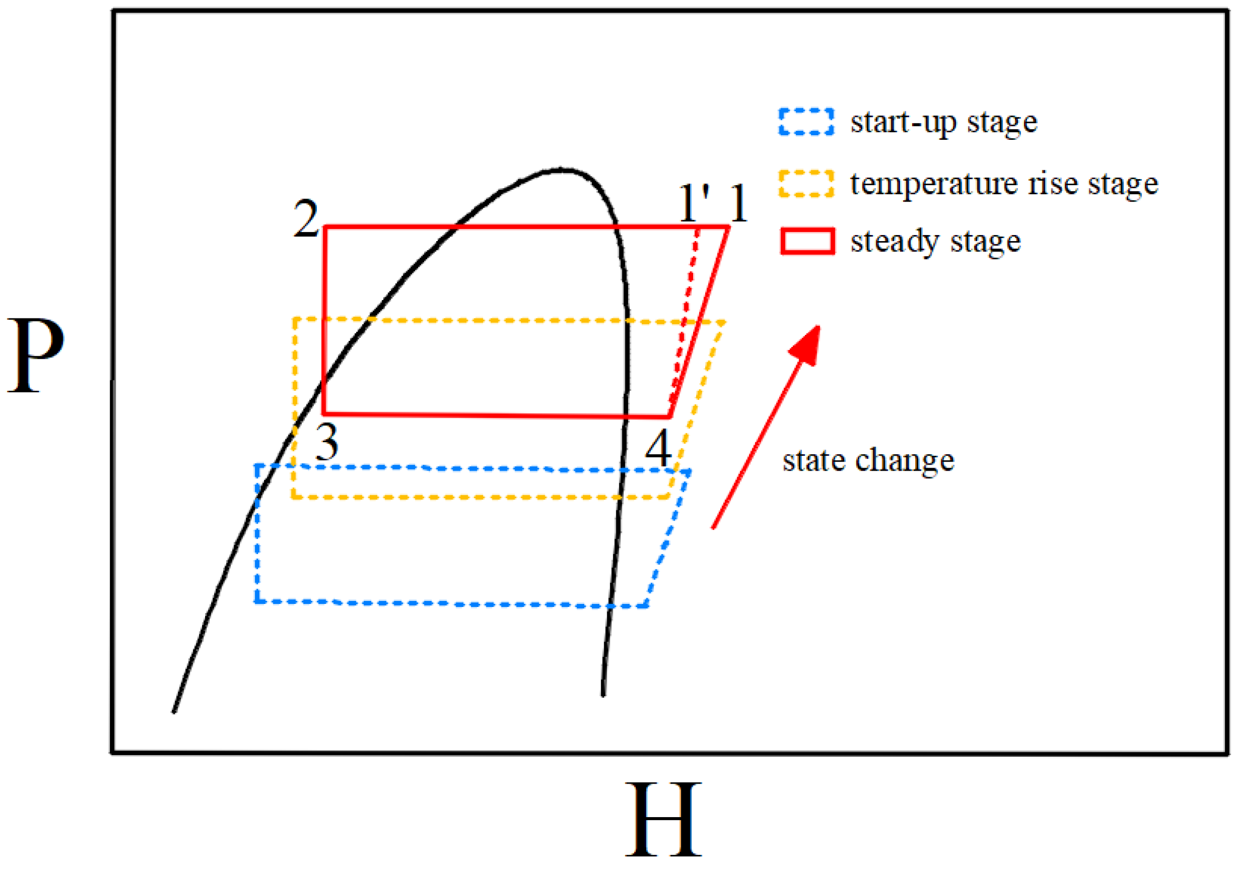
This section introduces the thermodynamic modeling framework of the HTHP, and Figure 7 shows the variation in the P-H diagram during HTHP operation. The HTHP cycle consists of four parts: vapor compression (4–1), condensation (1–2), the throttling process (2–3), and evaporation (3–4). By adjusting the compressor load and the electronic expansion valve opening, the HTHP system makes the thermodynamic cycle process change continuously. During the process, the evaporating and condensing temperatures constantly rise. Finally, the condensing temperature reaches the set temperature and remains stable.

The compressor isentropic efficiency η_s is given by Equation (4):

$${\eta }_{\mathrm{S}}={\displaystyle \frac{M_{\mathrm{ref}}\cdot (h_{1\prime }-h_4)}{W_{\mathrm{com}}}}$$

(4)

$$M_{\mathrm{ref}}={\displaystyle \frac{c_{\mathrm{p},\mathrm{w}}\cdot M_{\mathrm{source}}\cdot (T_{\mathrm{source},\mathrm{in}}-T_{\mathrm{source},\mathrm{out}})}{h_4-h_3}}$$

(5)

where h_i(i=1,2,3,4) is the unit mass refrigerant enthalpy at different state points in the heat pump cycle, and h_1′ is the unit mass refrigerant enthalpy obtained after isentropic compression. W_com is the output power of the compressor.

The compressor volumetric efficiency η_v is given by Equation (6):

$${\eta }_{\mathrm{v}}={\displaystyle \frac{3600\cdot M_{\mathrm{ref}}}{V_{\mathrm{stan}}\cdot {\rho }_{\mathrm{ref}}}}$$

(6)

where M_ref is the mass flow rate at the compressor suction port, V_stan is the rated suction volume of the compressor, ρ_ref is the refrigerant density at the compressor suction port, and C_p,w is the constant-pressure specific heat capacity of the refrigerant at the compressor suction port.

(ii)

Prediction model building

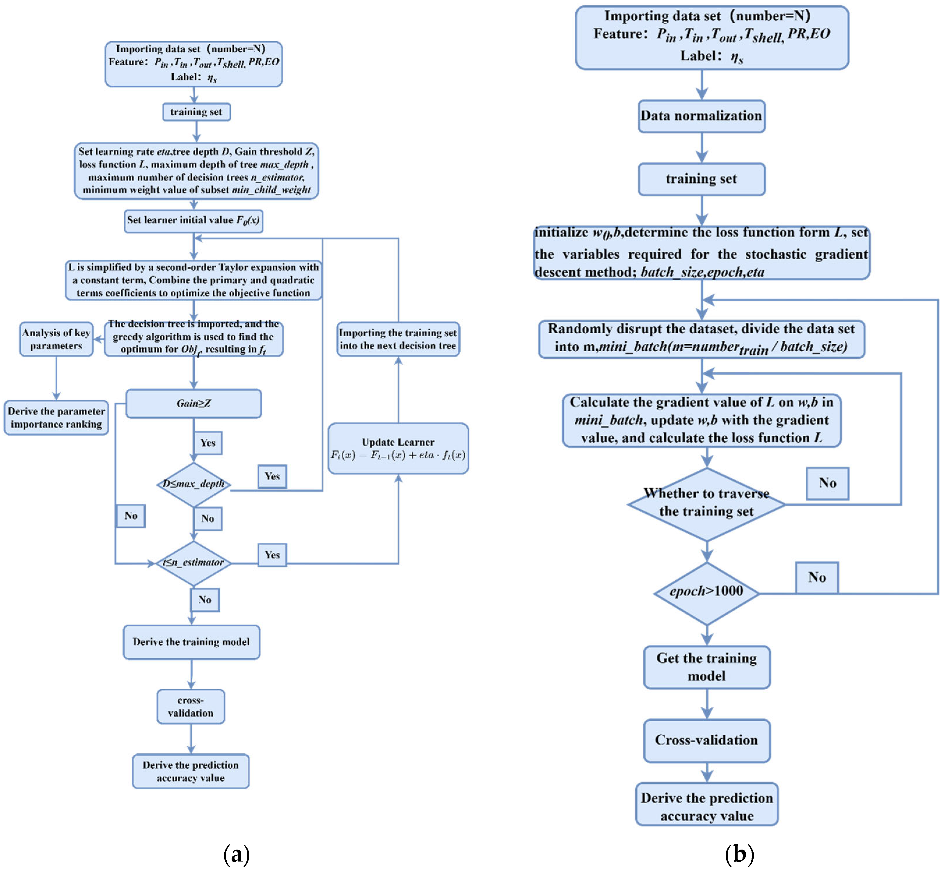
XGBoost is an optimization algorithm proposed by Tianqi Chen in 2016 based on the Gradient Boosting Decision Tree (GBDT), which can be used to analyze the importance of different variables and find key variables [34]. The specific process of XGBoost is shown in Figure 8a. In the process of optimal decision node selection, XGBoost analyzes the importance of different parameters by considering the number of key decisions made in the process of decision nodes. Parameter importance magnitude is calculated by the measurement of each attribute’s decision node improvement performance. The performance measure can be measured by the purity of the split points (Gini index) or other more specific error functions. In this work, the XGBoost model was built based on the XGBoost database in Python 2.7. The accuracy was measured using a cross-validation method with the gain threshold Z set to 0.5. The objective function search method used was the Greedy Algorithm.

The MLR model is one of the classic machine learning regression models and has been frequently used in the field of heat pumps. MLR has a simple structure and directly looks for linear combinatorial relationships between input variables to predict response values. The prediction is better when the relationship between the independent and dependent variables is linear. In this work, the MLR model was used in two places: (1) In key parameter identification, the original data were arranged according to the order of importance after XGBoost importance analysis. Then, the parameters were sequentially imported into the MLR model to test the rationality of key variables. (2) In the construction of empirical formula, after key parameters were identified, MLR was used to fit multiple linear regressions to the PR and the key parameters, and the cross-validation method was adopted for validation. This work used Python to build the MLR model, and the model used the stochastic gradient descent method to optimize the loss function. The learning rate (eta) was 0.01, and the number of training rounds (epoch) was 1000. The MLR flow block diagram is shown in Figure 8b.

2.2.2. Model Optimization

The model optimization part mainly used the TO method to reduce interaction between input parameters. The GS and BO algorithms were used to find the optimal hyperparameters of the XGBoost model. In this work, the input parameters were first preprocessed using TO to obtain data sets with more minor interactions. GS was mainly used to find the optimal value of the n_estimator in the XGBoost model; the test index was variance, as shown in Equation (7). The variance reflects the effect on the stability of the prediction accuracy. BO was based on Bayes’ theorem, and the optimal hyperparameters were found by constructing a probabilistic model of the objective function. After obtaining the optimal value of n_estimator, BO was mainly used to find the maximum depth of the decision tree. It is primarily used to find the optimal deals of four hyperparameters: max_depth, eta, gamma, and min_child_weight of the subset. The R² obtained from cross-validation was considered as the accuracy validation standard for the optimized model, as shown in Equation (8).

$$variance={\displaystyle \frac{{\displaystyle {\sum }_{x\in D}{(\widehat{f}(x)-\stackrel{-}{\widehat{f}(x)})}^2}}{N-1}}$$

(7)

$$R^2=1-{\displaystyle \frac{{{\displaystyle {\sum }_{x\in D}(\widehat{f}(x)-f(x))}}^2}{{\displaystyle {\sum }_{x\in D}{(\widehat{f}(x)-\stackrel{-}{\widehat{f}(x)})}^2}}}$$

(8)

where D is the data set, and n is the number of samples in the data set.

2.3. Key Parameter Identification and Isentropic Efficiency Empirical Formula Construction

After obtaining reliable data and a prediction model, the identification of key parameters and the construction of the empirical formulas were carried out. The key parameter identification work started with parameter importance analysis based on a high-prediction-accuracy XGBoost model. Then, based on the analysis results, an exhaustive analysis of parameters was performed using the MLR model. The contribution of the parameters to the accuracy of the prediction was analyzed and calibrated to determine the key parameters. The empirical formulas were then constructed based on the key parameters obtained from the model analysis and the PR from previous research. This construction process used the MLR algorithm to construct empirical formulas for multi-order isentropic efficiency. The best empirical formulas were selected by combining R² and formula complexity considerations. Finally, the generalizability of the empirical formulas was verified by experimental data from other researchers, and the feasibility of the method was also discussed.

3. Results and Discussion

3.1. Data Processing and Parameter Screening

Based on the original data and the preliminary screening parameters, the Mahalanobis distance method was used to detect abnormal values in the data, combined with the judgment of basic engineering principles. In total, 2343 sets of data were identified for the data labeling values for isentropic efficiency, and 2081 sets of data were identified for the data labeling values for isentropic efficiency.

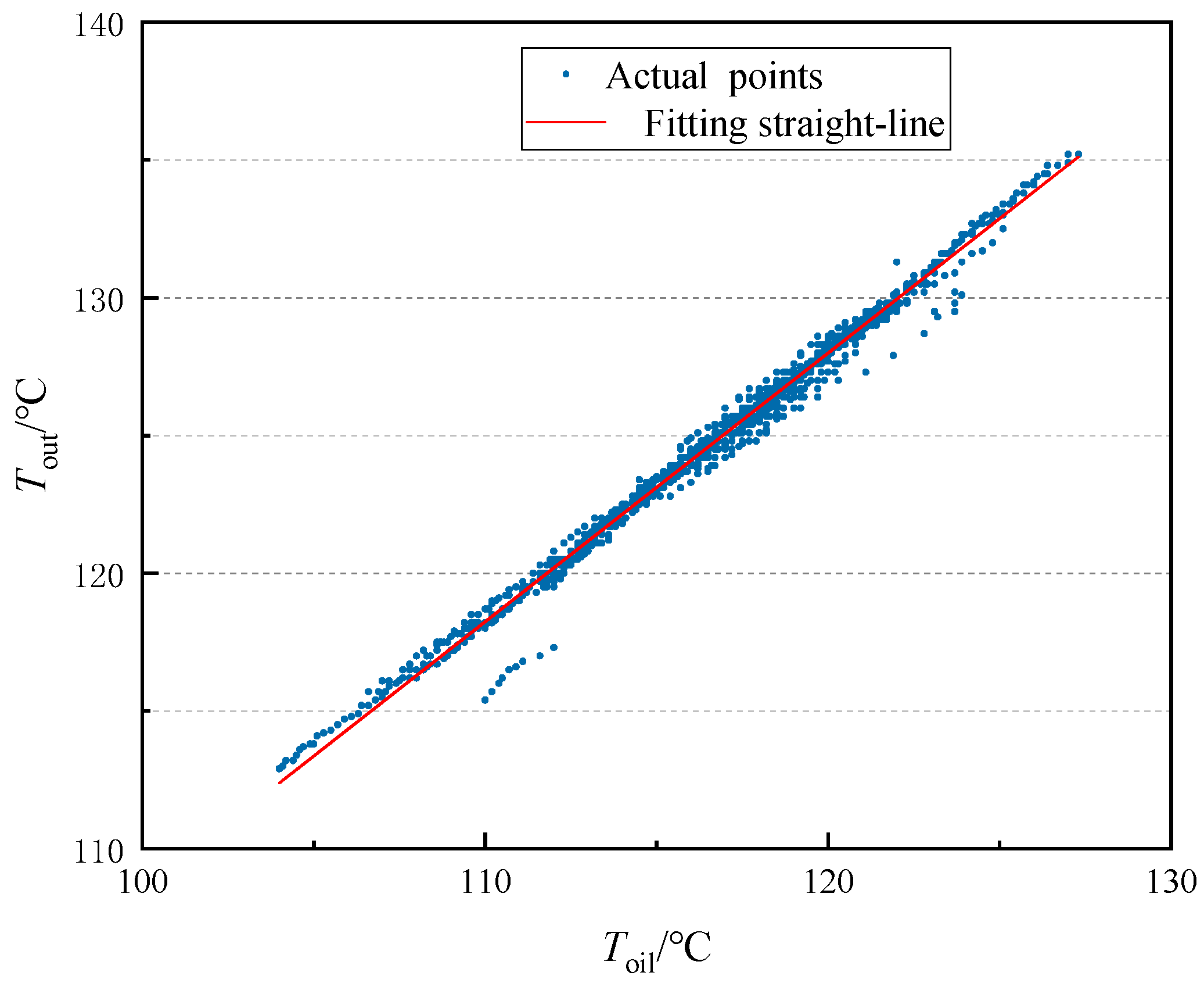
The uncertainty analysis was then performed for the performance indicators of the HTHP system. The results are shown in

Table 7. Uncertainty analysis of performance parameters.

	ηs	ηv
maximum	0.0243	0.0296
minimum	0.0226	0.0266
average	0.0232	0.0277
relative measurement uncertainty	0.0558	0.0587

. From the results of the uncertainty analysis, it can be determined that the collected data had good stability and was less affected by factors such as the accuracy of the collection equipment. On this basis, correlation analysis was used to analyze the interaction of parameters to optimize collinearity problems between input parameters. The Pearson coefficient between T_oil and T_out was found to be 0.995, much larger than the correlation performance of other parameters, as shown in Figure 9. Based on the analysis of the principle of the oil cooling cycle for twin-screw compressors, it was found that the heat exchange process of lubricating oil and gaseous refrigerant was closely combined, resulting in the temperature change process being very similar. One of the variables could be selected when conducting the subsequent analysis. In this work, T_out was the input variable for the following reasons: (1) T_out is the temperature at the outlet near the compression chamber. At the same time, T_oil is the temperature at the compression tank far from the room. T_out can more accurately reflect the temperature of the compression process inside the compressor. (2) T_out is more informative; most current researchers use T_out as an operating parameter, and T_oil is used as an operational parameter in fewer cases. The final determination of the input parameters and their ranges are shown in

Table 8. Screened parameters and their ranges.

	Pin (bar)	Pout (bar)	Tin (°C)	Tout (°C)	EO (%)	Tshell (°C)	ΔToverheat,in	ΔToverheat,out
Min	2.4	11.6	42.1	96.4	29.8	41.6	0.1	0.1
Max	4.8	21.9	68.5	131.7	100.0	67.9	10.5	8.5

. The remaining parameters responded to a certain degree of interaction between them. But the decision tree principle in the XGBoost algorithm and the optimization procedure designed within the algorithm can cope with these problems and achieve accurate prediction results.

3.2. Optimization of Model

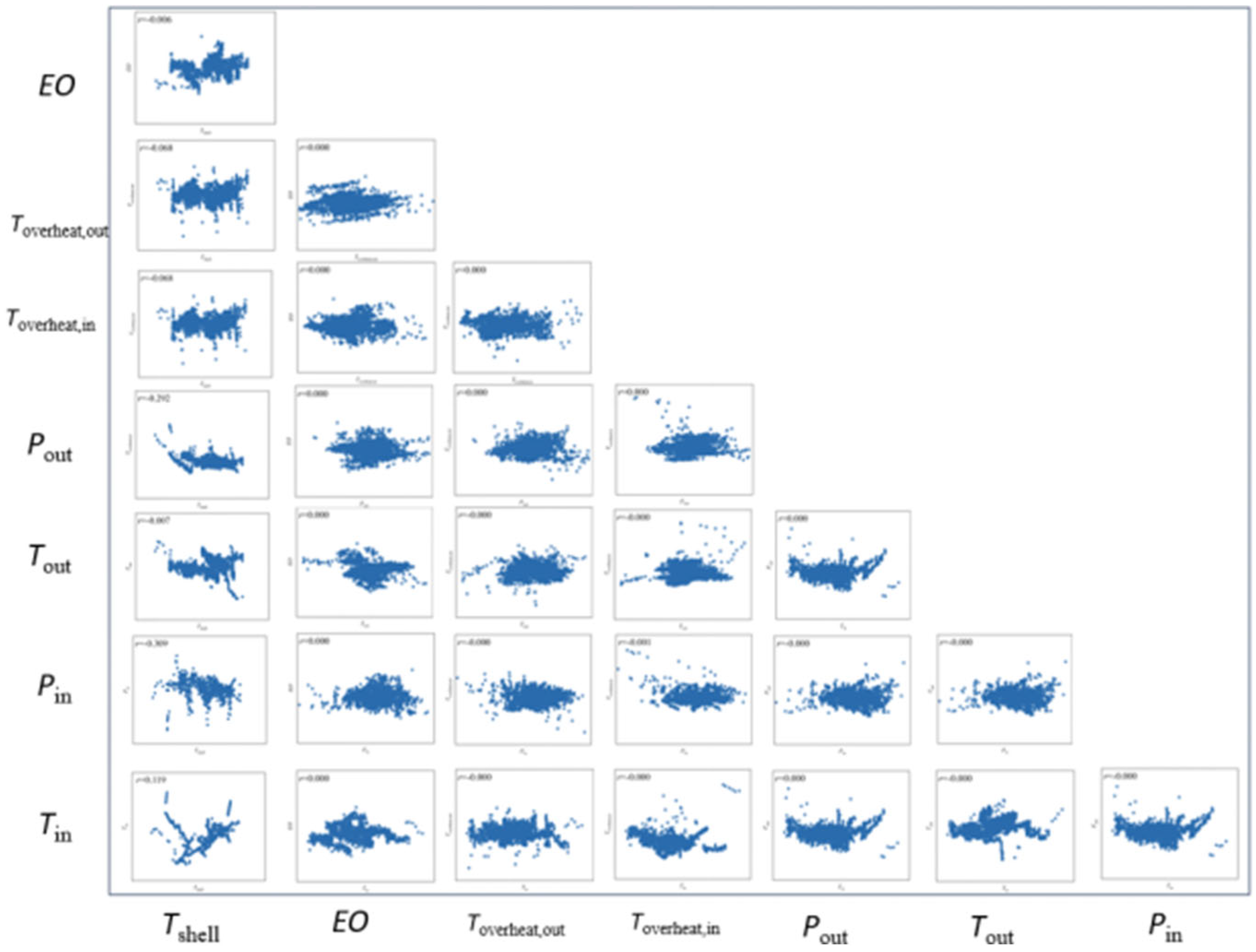
Despite combining the actual physical interaction through the correlation analysis in Section 3.1, the significant interaction between T_out and T_oil was eliminated. However, there is some correlation between the remaining parameters of the model. If the model is entered directly, it will have an impact on the model significance analysis. Orthogonal transformation (OT) transforms the original features into a set of orthogonal features, thus reducing the correlation between them. Orthogonal transformations were performed on the eight input parameters shown in Table 8. After OT, the correlation relationship between the parameters is shown in Figure 10. The results shown that the Pearson coefficient between T_shell and T_in, P_in, T_out, P_out, T_overheat,in, T_overheat,out, and EO is 0.119, 0.309, 0.007, 0.292, 0.068, 0.068, and 0.006, respectively. The Pearson coefficient of EO, T_in, P_in, T_out, P_out, T_overheat,in, and T_overheat,out with other parameters is almost always zero. All the above indicate that there was no significant correlation among these seven parameters, which were regarded as the key parameters for fitting the isentropic and volumetric efficiencies.

In the hyperparameter optimization process of the prediction model, since the n_estimator had a significant influence on other hyperparameters of the XGBoost algorithm, the optimal value of the n_estimator of the XGBoost decision tree was searched by the GS first. Then, BO was used to find the optimal values of the four hyperparameters max_depth, eta, gamma, and min_child_weight, and its accuracy was verified by using R² obtained by the cross-validation method to obtain the best value.

As shown in Figure 11, when isentropic efficiency was used as the model labeling value, the optimal hyperparameters obtained after grid search and Bayesian optimization were n_estimator, 217; max_depth, 6; eta, 0.04453; gamma, 0.006822; and min_child_weight, 6.666. With the above hyperparameter settings, the resulting R² was 0.9581. As shown in Figure 12, when volumetric efficiency was used as the model labeling value, the optimal hyperparameters obtained after grid search and Bayesian optimization were n_estimator, 226; max_depth, 5; eta, 0.04176; gamma, 0.006868; and min_child_weight, 8.003. With the above hyperparameter settings, the resulting R² was 0.9678. Through the above calculation, an optimization model is obtained, which is convenient in carrying out follow-up research.

3.3. Key Parameters of XGBoost-MLR Algorithm Analysis

The XGBoost algorithm performs the importance analysis of parameters in terms of the number of key decisions that they make. This importance analysis can be used to derive the degree of influence of other features on the label values. The results are reflected by the F-value, The larger the F-value, the greater the importance of its features. Figure 13a shows the results of XGBoost importance analysis with parameters and η_s as the label value. Figure 13b shows the results of XGBoost importance analysis with parameters and η_v as the label value.

Figure 13a shows that the F-values are ordered from largest to smallest: T_overheat,in, T_in, T_out, P_out, T_shell, EO, P_in, T_overheat,out, P_in. More specifically, the F-values of T_overheat,in, T_in, and T_out are significantly larger than those of the other variables, indicating that temperature variables play a more important role in the prediction model training process. Figure 13b shows that the F-values are ordered from largest to smallest: T_out, T_overheat,in, T_in, T_shell, T_overheat,out, P_out, P_in, and EO. The graph likewise reflects the importance of the temperature parameters: T_overheat,in, T_in, and T_out.

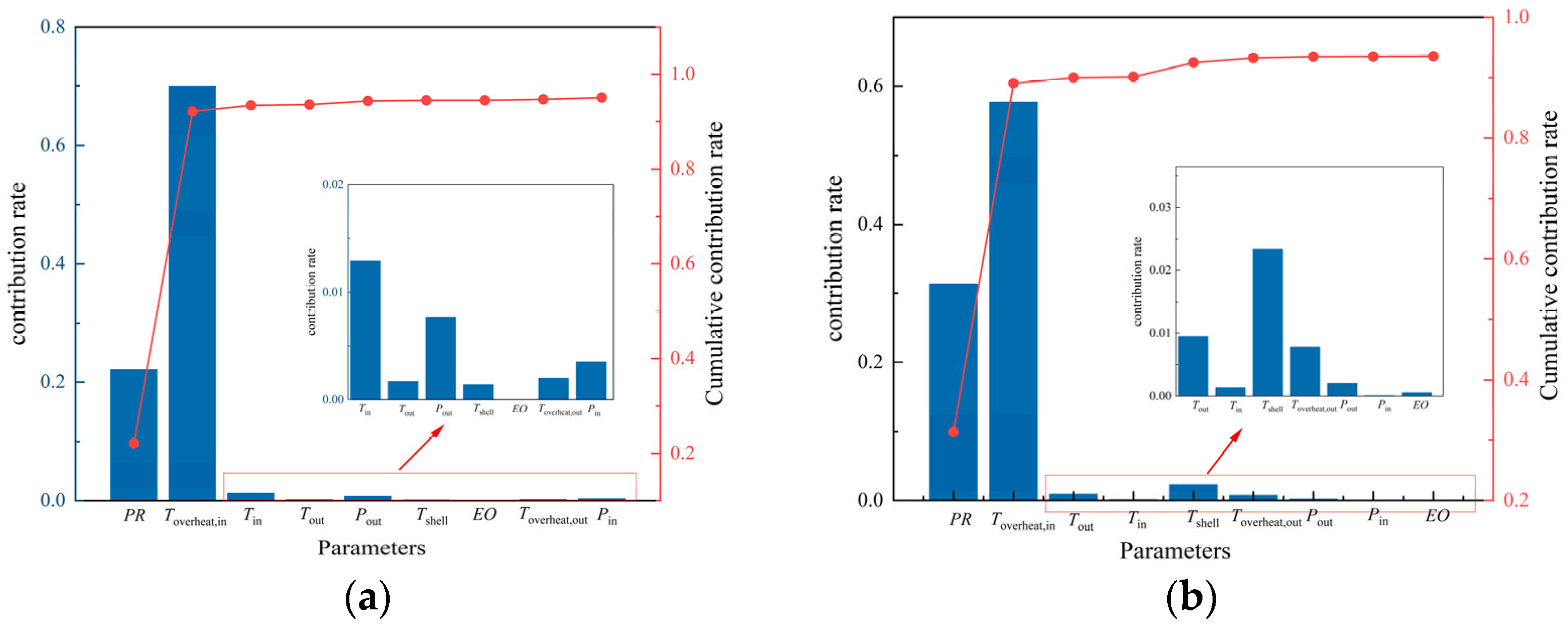
As summarized above, the isentropic efficiency and volumetric efficiency of an HTHP and its influencing parameters are still dominated by a linear relationship. PR is an important parameter commonly found by previous researchers. In this work, the construction of the empirical equation was still based on establishing a linear polynomial. Therefore, it is feasible to use the MLR algorithm for key parameter identification. Based on the original important parameter PR, the importance of each parameter was assessed in terms of its contribution to the predicted R². Precisely, referring to the order of importance analysis, the parameters were verified by exhaustion using the MLR algorithm as the method.

The final values and cumulative contributions of the parameters to the model prediction R² as the model input parameters increase are shown in Figure 14. Figure 14a shows that R² could reach 92.12% when PR, T_overheat,in were the input parameters of the MLR model in the temperature range of 115~133 °C, while the contribution of the remaining parameters was minimal (2.92% in total). To ensure the simplicity of the subsequent empirical formulas, PR, T_overheat,in can be identified as the key variables, and the effect of temperature variables on isentropic efficiency can be determined. Figure 14b shows that R² could reach 89.05% when PR, T_overheat,in were the input parameters of the MLR model in the temperature range of 115~133 °C, while the contribution of the remaining parameters was minimal (4.49% in total). PR, T_overheat,in can be identified as the key variables, and the effect of temperature variables on isentropic efficiency can be determined.

3.4. Fitting and Analysis of Empirical Equation Based on Key Parameters

Based on the identification results of the above key parameters, it can be confirmed that PR, T_overheat,in are the key parameters for isentropic efficiency and volumetric efficiency. Next, the empirical equations for the isentropic efficiency and volumetric efficiency will be established. It is necessary to clarify the establishment of the isentropic efficiency empirical formulas based on the following premises:

(1)

The compressor used was a semi-hermetic twin-screw compressor.

(2)

The process complied with the operating range of data determined in

Table 9. The range of variable parameters.

Parameters	Lower Limit	Upper Limit	Range Width
Tout/°C	95	135	40
PR	3	8	5
Tin/°C	40	70	30
Toverheat,in/°C	1	10	9
Toverheat,out/°C	1	8	7
ηs	0.2	0.8	0.6
ηv	0.2	0.8	0.6

.

Based on the analysis of key parameters, this paper adopts the MLR to carry out multiple linear regression fitting with key parameters as variables. Linear polynomials of first-order, second-order, third-order, and fourth-order accuracy were fitted separately to find the best-fitting formula. The fitted polynomials were cross-validated with a validation fold of 5, and R² was used as the judging index of the appropriate accuracy. The specific fits are shown in

Table 10. Fitting equations and their R².

Number of Orders	First-Order Equation	Second-Order Equation	Third-Order Equation	Fourth-Order Equation
Formula type	$y={\displaystyle \sum _{i=1}^3{a}_i{x}_i}+d$	$y={\displaystyle \sum _{i=1}^3{a}_i{x}_i}+{\displaystyle \sum _{i=1}^3{b}_i{x_i}^2}+d$	$y={\displaystyle \sum _{i=1}^3{a}_i{x}_i}+{\displaystyle \sum _{i=1}^3{b_i{x}_i}^2}+{\displaystyle \sum _{i=1,j\ne i}^3{c_i{x}_i}^3}+d$	$y={\displaystyle \sum _{i=1}^3{a}_i}{x}_i+{\displaystyle \sum _{i=1}^3{b}_i}{x_i}^2+{\displaystyle \sum _{i=1}^3{c}_i}{x_i}^3+{\displaystyle \sum _{i=1}^3{d}_i}{x_i}^4+e$
Isentropic efficiency formula (R2)	0.9212	0.9510	0.9547	0.9587
Volumetric efficiency formula (R2)	0.8905	0.9129	0.9138	0.9157

.

As can be seen from the relevant results, the first-order formula had the lowest accuracy in the empirical equations for isentropic and volumetric efficiency. Second-order formulas were significantly more accurate than first-order formulas. When the order was higher than second order, the increase in order had a weak effect on accuracy. However, the increase in order led to an increase in the complexity of the formulas. So, the second-order formula was chosen for the isentropic efficiency and volumetric efficiency. The final isentropic efficiency empirical formula is shown in the following equation:

$${\eta }_s=0.106+0.09398PR+0.08075T_{\mathrm{overheat},\mathrm{in}}-0.014211P{R}^2-0.002836T_{\mathrm{overheat},\mathrm{in}}^2$$

(9)

$${\eta }_v=0.4245-0.0630PR+0.10760T_{\mathrm{overheat},\mathrm{in}}+0.00162P{R}^2-0.004449T_{\mathrm{overheat},\mathrm{in}}^2$$

(10)

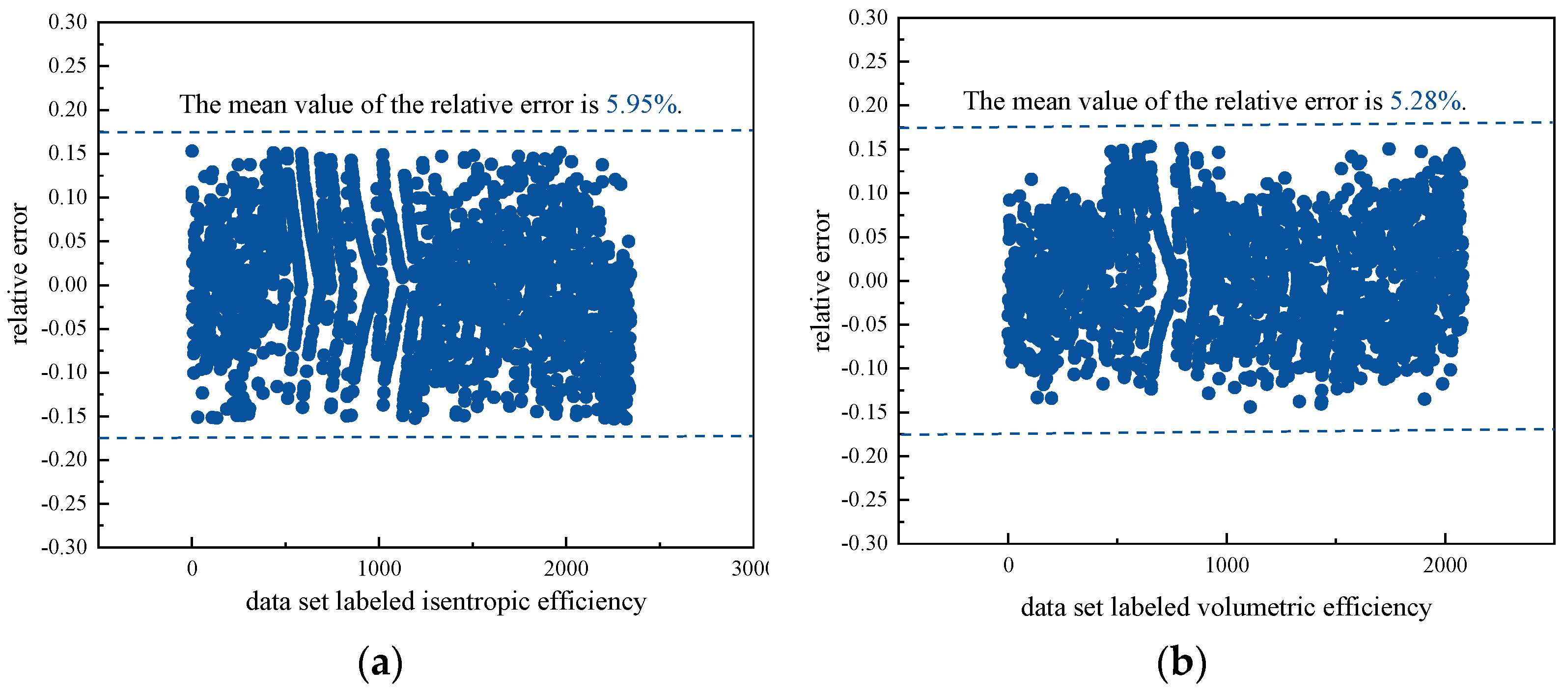
The fitted values of η_s and η_v were calculated by the fitting formula and compared with the actual value. At the same time, the relative error was used as an evaluation index. The comparison results are shown in Figure 15.

As shown in Figure 15, The relative errors of the isentropic efficiency empirical formula are between −15.3% and 15.2%. The mean value of the relative errors is 5.95%, which indicates accurate performance by the empirical formulas. As shown in Figure 15, the relative errors of the volumetric efficiency empirical formula are between −14.4% and 15.3%. The mean value of the relative errors is 5.28%, which can achieve a good fitting effect.

Based on the proposed empirical equations, the isentropic and volumetric efficiency performances are analyzed under different conditions. The specific changes are shown in Figure 16. The following conclusions can be drawn from the graph:

(1)

Within a limited range of PR, the system η_s and η_v basically decrease with increasing PR, which is consistent with the trend obtained by the previous researcher. When PR is less than 4, the isentropic efficiency does not change significantly with PR. For example, when the compression ratio is changed from 3.5 to 4, the change in system isentropic efficiency is only 0.006301. The isentropic efficiency increases the decay rate with increasing compression ratio. On the contrary, the volumetric efficiency decreases the decay rate with increasing compression ratio.

(2)

Within a limited range of T_overheat,in, the system η_s and η_v increase with increasing T_overheat,in. T_overheat,in has a contributory effect on system performance. Changes in performance parameters due to changes in T_overheat,in can be explained from a physical point of view: the increase in T_overheat,in makes the inhaled gas more stable and reduces the liquid component in it. The actual suction volume of the compressor is closer to the theoretical value. As a result, volumetric efficiency losses due to gas–liquid mixtures are reduced, and compressor power consumption due to liquid strikes in the compressor is minimized.

3.5. Validation of the Generalizability of the Empirical Formulas and Explanation of Method Generalizability

To verify the correctness and generalizability of the empirical formulas, the experimental data of HTHPs from different researchers were used in this work for validation. The experimental data from specific researchers and the validation results proposed in this work are shown in

Table 11. Details of the data used for validation.

Researchers	Refrigerant	Compressor Type	Exhaust Temperature Range (°C)	Relative Error of Isentropic Empirical Formula (%)	Relative Error of Volumetric Empirical Formula (%)
Zhao [12]	R717	Twin-Screw Compressors	75~90	5.25	9.43
Zhuang [35]	R245fa	Twin-Screw Compressors	90~105	1.92	15.9
Zhang [36]	R245fa	Twin-Screw Compressors	90~115	4.16	2.84
Ma [37]	R245fa	Reciprocating Compressors	80~102	28.7	N/A
Ma [38]	R245fa	Scroll Compressors	110~147	16.53	6.43

.

As can be seen from Table 11, the proposed empirical formulas have a clear range of applicability. The empirical formulas apply to a clear range of compressor types. Twin-screw compressors have the highest applicability, while scroll compressors and reciprocating compressors have low applicability. From the experimental data, it can be seen that the relative error of the experimental data of both of them is more than 15%. The empirical formulas are also applicable to other refrigerants under twin-screw compressor conditions. For example, when using R717 refrigerant, the isentropic and volume efficiency empirical formula of the relative error is less than 10%. At the same time, the volumetric efficiency performance is significantly affected by the refrigerant charge in the heat pump system, the physical structure of the compressor, etc. Therefore, the applicability of the empirical formula for volumetric efficiency is unstable in compressors of different sizes. As shown in the table, Zhuang used a twin-screw compressor and was in the appropriate temperature range [35]. However, the relative error between the experimental data and the volumetric efficiency empirical formula is more than 15%. In contrast, the empirical equations for isentropic efficiency are more widely applicable. As can be seen from the table, the relative error of the empirical equations for isentropic efficiency is always low under the condition of a twin-screw compressor.

The key parameter identification and empirical formula construction methods proposed in this work are also generalizable. On the one hand, they are based on the data obtained from the HTHP experiment system. The selection of input parameters is based on basic thermodynamic knowledge as well as the operating principle of the HTHP units. The method of selecting parameters is universal for general vapor compression HTHP systems. On the other hand, the XGBoost and MLR algorithms are well-established models with application examples in thermal engineering. Although the MLR model has a linear relationship requirement for the variables, it corresponds to the linear polynomial of the final constructed empirical formula. Finally, the data processing methods used, including correlation analysis, TO, GS, BO, and other processing methods, do not have strict requirements for the original data. Therefore, the method is generalizable when analyzed in terms of the whole process. However, the current situation still makes testing the methodology through real data difficult. A large amount of real and stable experimental data on HTHPs is needed, which is also characteristic of the data-driven methodology. The follow-up work will involve building a new high-temperature heat pump unit to verify the generalizability of the methodology.

4. Conclusions

This work proposed a method for identifying key parameters of the isentropic and volumetric efficiency based on machine learning algorithms. The data source is a 60 kW industrial-grade HTHP. The XGBoost-MLR algorithm was used to identify key parameters. The model used TO, CV, and BO algorithms as optimization means to ensure the accuracy of parameter identification. Then, the empirical formulas for isentropic and volumetric efficiency were reconstructed based on the identified key parameters. Finally, the generalizability of the empirical formulas and the feasibility of the method was discussed. The main conclusions are as follows:

(1)

The model established by the XGBoost-MLR algorithm can accurately identify the key parameters of HTHPs in a limited temperature range. Using the OT algorithms can effectively optimize the input parameter collinearity problem. CV and BO algorithms can improve the prediction model accuracy and make the model R² stable above 0.95.

(2)

In the specified high-temperature range of 90~132 °C, the key parameters of isentropic and volumetric efficiency are PR, T_overheat,in, which can be used to achieve high prediction accuracy. Deleting the key parameters will lead to a significant decrease in the accuracy of the prediction model.

(3)

The empirical formulas of the isentropic and volumetric efficiency constructed based on the key parameters have high accuracy in the temperature range. The relative error of isentropic efficiency empirical formula is between −15.3% and 15.2%. The mean value of the relative errors is 5.95%. The relative error of the volumetric efficiency empirical formula is between −14.4% and 15.3%. The mean value of the relative errors is 5.28%.

(4)

The system η_s and η_v basically decrease with increasing PR. However, when PR is less than 4, the isentropic efficiency does not change significantly with PR. The system η_s and η_v increase with increasing T_overheat,in.

(5)

The proposed empirical formulas have a clear range of applicability. Twin-screw compressors have the highest applicability. The relative error of the experimental data of scroll compressors and reciprocating compressors is more than 15%. The applicability of the empirical formula for volumetric efficiency is unstable in compressors of different sizes. In contrast, the empirical equations for isentropic efficiency are more widely applicable. The method is generalizable when analyzed in terms of the whole process, which includes the selection of input parameters, the algorithms, and the optimization methods.

In future work, we plan to introduce further advanced machine learning algorithms such as neural networks to improve the prediction accuracy and anti-interference ability of the model and consider its strategy to control the influence of parameters such as superheat and model flow. We will then further explore the control strategy of the model to improve its performance.

References

1. United Nations Bureau. National Statistical Yearbook 2022 [EB/OL]. 13 October 2022. Available online: https://www.stats.gov.cn/sj/ndsj/2022/indexch.htm (accessed on 12 May 2023).
2. Yan, H.; Hu, B.; Wang, R. Air-source heat pump for distributed steam generation: A new and sustainable solution to replace coal-fired boilers in China. Adv. Sustain. Syst. 2020, 4, 2000118. [Google Scholar] [CrossRef]
3. Arpagaus, C.; Bless, F.; Uhlmann, M.; Schiffmann, J.; Bertsch, S.S. High-temperature heat pumps: Market overview, state of the art, research status, refrigerants, and application potentials. Energy 2018, 152, 985–1010. [Google Scholar] [CrossRef]
4. Jiang, J.; Hu, B.; Wang, R.; Deng, N.; Cao, F.; Wang, C.-C. A review and perspective on industry high-temperature heat pumps. Renew. Sustain. Energy Rev. 2022, 161, 112106. [Google Scholar] [CrossRef]
5. Kaida, T.; Sakuraba, I.; Hashimoto, K.; Hasegawa, H. Experimental performance evaluation of heat pump-based steam supply system. In Proceedings of the 9th International Conference on Compressors and their Systems, London, UK, 5–9 September 2015. [Google Scholar] [CrossRef]
6. Ochsner, K. High-temperature heat pumps for waste heat recovery. In Proceedings of the 8th EHPA European Heat Pump Forum, Brussels, Belgium, 8 May 2015; pp. 1–10. [Google Scholar]
7. Zauner, F. Hochtemperatur-Wärmepumpen zur energetischen Nutzung industrieller (Niedertemperatur-) Abwärme, Ochsner Energie Technik GmbH. In Proceedings of the Highlights der Energieforschung 2016, Die Rolle der Wärmepumpe im zukünftigen Energiesystem, Vienna, Austria, 22 June 2016; pp. 1–11. [Google Scholar]
8. Jensen, J.K.; Ommen, T.; Markussen, W.B.; Reinholdt, L.; Elmegaard, B. Technical and economical working domains of industrial heat pumps: Part 2–Ammonia-water hybrid absorption-compression heat pumps. Int. J. Refrig. 2015, 55, 183–200. [Google Scholar] [CrossRef]
9. Dietrich, W.; Fredrich, O. GEA Grasso Heat Pumps Using Ammonia—The Megawatt Range; Achema: Frankfurt, Germany, 2012. [Google Scholar]
10. Nilsson, M.; Rislå, H.N.; Kontomaris, K. Measured performance of a novel high-temperature heat pump with HFO-1336mzz (Z) as the working fluid. In Proceedings of the 12th IEA Heat Pump Conference, Rotterdam, The Netherlands, 15–18 May 2017. [Google Scholar]
11. Wang, K.; Cao, F.; Xing, Z. Development and experimental validation of a high-temperature heat pump for heat recovery and building heating. Energy Build. 2009, 41, 732–737. [Google Scholar] [CrossRef]
12. Zhao, Z.; Xing, Z.; Hou, F.; Tian, Y.; Jiang, S. Theoretical and experimental investigation of a novel high-temperature heat pump system for recovering heat from refrigeration system. Appl. Therm. Eng. 2016, 107, 758–767. [Google Scholar] [CrossRef]
13. Afshari, F.; Comakli, O.; Lesani, A.; Karagoz, S. Characterization of lubricating oil effects on the performance of reciprocating compressors in air–water heat pumps. Int. J. Refrig. 2017, 74, 505–516. [Google Scholar] [CrossRef]
14. Wu, D.; Jiang, J.; Hu, B.; Wang, R. Experimental investigation on the performance of a very high temperature heat pump with water refrigerant. Energy 2020, 190, 116427. [Google Scholar] [CrossRef]
15. Chamoun, M.; Rulliere, R.; Haberschill, P.; Peureux, J.-L. Modelica-based modeling and simulation of a twin screw compressor for heat pump applications. Appl. Therm. Eng. 2013, 58, 479–489. [Google Scholar] [CrossRef]
16. Zhang, X.; Xu, H. Experimental performance of moderately high temperature heat pump with working fluid R1234ze(Z). J. Therm. Anal. Calorim. 2021, 144, 1535–1545. [Google Scholar] [CrossRef]
17. Sulaiman, A.Y.; Cotter, D.F.; Le, K.X.; Huang, M.J.; Hewitt, N.J. Thermodynamic analysis of subkey High-Temperature heat pump using low GWP Refrigerants: A theoretical evaluation. Energy Convers. Manag. 2022, 268, 116034. [Google Scholar] [CrossRef]
18. Zhang, S.-J.; Wang, H.-X.; Guo, T.; Chen, C. Performance Simulation and Experimental Testing of Moderately High Temperature Heat Pump Using Non-azeotropic Mixture for Geothermal District Heating. In Proceedings of the 2010 Asia-Pacific Power and Energy Engineering Conference, Chengdu, China, 28–31 March 2010. [Google Scholar]
19. Wang, G.; Zhang, X. Thermoeconomic analysis of optimization potential for CO2 vapor compression cycle: From transkey to superkey operation for waste heat recovery from the steam condenser. Int. J. Energy Res. 2019, 43, 297–312. [Google Scholar] [CrossRef]
20. Chamoun, M.; Rulliere, R.; Haberschill, P.; Peureux, J.-L. Experimental and numerical investigations of a new high temperature heat pump for industrial heat recovery using water as refrigerant. Int. J. Refrig. 2014, 44, 177–188. [Google Scholar] [CrossRef]
21. Wang, L.; Hou, Z.; LI, X.; Feng, L.; Song, M. Study on characteristics of high-temperature hybrid heat pump system for boiling water heater with different refrigerants. J. Therm. Sci. Technol. 2022, 21, 83–90. [Google Scholar] [CrossRef]
22. Guth, T.; Atakan, B. Semi-empirical model of a variable speed scroll compressor for R-290 with the focus on compressor efficiencies and transferability. Int. J. Refrig. 2023, 146, 483–499. [Google Scholar] [CrossRef]
23. Tian, X.; Hao, Y.; Zhao, G.; Liang, J. Research on Dynamic Modeling of a High Temperature Steam Heat Pump. In Proceedings of the 2020 Chinese Automation Congress (CAC 2020), Shanghai, China, 6–8 November 2020. [Google Scholar] [CrossRef]
24. Roskosch, D.; Venzik, V.; Atakan, B. Thermodynamic model for reciprocating compressors with the focus on fluid dependent efficiencies. Int. J. Refrig. 2017, 84, 104–116. [Google Scholar] [CrossRef]
25. Negrão, C.O.; Erthal, R.H.; Andrade, D.E.; da Silva, L.W. A semi-empirical model for the unsteady-state simulation of reciprocating compressors for household refrigeration applications. Appl. Therm. Eng. 2011, 31, 1114–1124. [Google Scholar] [CrossRef]
26. Threlkeld, J.L. Thermal Environmental Engineering; Prentice-Hall: Englewood Cliffs, NJ, USA, 1962. [Google Scholar]
27. Li, W. Simplified steady-state modeling for variable speed compressor. Appl. Therm. Eng. 2013, 50, 318–326. [Google Scholar] [CrossRef]
28. Ye, K.K.; Demirezen, G.; Fung, A.S.; Janssen, E. The use of artificial neural networks (ANN) in predicting the energy consumption of air-source heat pump in retrofit residential housing. In Proceedings of the IOP Conference Series: Earth and Environmental Science, Xiamen, China, 11–19 November 2020; IOP Publishing: Bristol, UK, 2020. [Google Scholar]
29. Miao, Z. Intelligent control system for the electric vehicle heat pump air conditioner based on machine learning. Front. Energy Res. 2023, 11, 1142243. [Google Scholar] [CrossRef]
30. Noye, S.; Martinez, R.M.; Carnieletto, L.; De Carli, M.; Aguirre, A.C. A review of advanced ground source heat pump control: Artificial intelligence for autonomous and adaptive control. Renew. Sustain. Energy Rev. 2022, 153, 111685. [Google Scholar] [CrossRef]
31. Yan, D.; Yang, F.; Yang, F.; Zhang, H.; Guo, Z.; Li, J.; Wu, Y. Identifying the key system parameters of the organic Rankine cycle using the principal component analysis based on an experimental database. Energy Convers. Manag. 2021, 240, 114252. [Google Scholar] [CrossRef]
32. Huang, Y.; Yuan, Y.; Chen, H.; Wang, J.; Guo, Y.; Ahmad, T. A novel energy demand prediction strategy for residential buildings based on ensemble learning. Energy Procedia 2019, 158, 3411–3416. [Google Scholar] [CrossRef]
33. De Maesschalck, R.; Jouan-Rimbaud, D.; Massart, D.L. The mahalanobis distance. Chemom. Intell. Lab. Syst. 2000, 50, 1–18. [Google Scholar] [CrossRef]
34. Chen, T.; Guestrin, C. Xgboost: A scalable tree boosting system. In Proceedings of the 22nd acm Sigkdd International Conference on Knowledge Discovery and Data Mining, San Francisco, CA, USA, 13–17 August 2016. [Google Scholar] [CrossRef]
35. Zhuang, X.; Guo, J.; Sun, J.; Zhao, X.; Bao, S. Experimental research on the cyclic Performance of High-Temperature Heat Pump with R134a/R245fa in comparison with R245fa. J. Qingdao Univ. Technol. 2020, 41, 81–86. [Google Scholar]
36. Zhang, T.; Shi, P.; Shao, X.; Liu, P.; Zhao, Y. Experimental Study on High Temperature Heat Pump Unit Based on R245fa Working Fluid. Mech. Electr. Inf. 2020, 25, 82–85. [Google Scholar] [CrossRef]
37. Ma, L.; Wang, H.; Wang, J. Cycle performance evaluation of HFC245fa for high-temperature heat pump systems. Acta Energiae Solaris Sin. 2010, 31, 749–753. [Google Scholar] [CrossRef]
38. Ma, X.; Zhang, Y.; Fang, L.; Yu, X.; Li, X.; Sheng, Y.; Zhang, Y. Performance analysis of a cascade high temperature heat pump using R245fa and BY-3 as working fluid. Appl. Therm. Eng. 2018, 140, 466–475. [Google Scholar] [CrossRef]
Figure 1. The required temperatures in different industrial fields.
Energies 18 04454 g001
Figure 2. Methodology of this article.
Energies 18 04454 g002
Figure 3. Equipment structure diagram of the system.
Energies 18 04454 g003
Figure 4. Scene diagram of the experimental test.
Energies 18 04454 g004
Figure 5. Instantaneous flow rate in the heat source of the system.
Energies 18 04454 g005
Figure 6. Oil-cooled cycle of the twin-screw compressor.
Energies 18 04454 g006
Figure 7. The P-H diagram of the system operation process.
Energies 18 04454 g007
Figure 8. Principles of MLR model and XGBoost model. (a) MLR model (b) XGBoost model.
Energies 18 04454 g008
Figure 9. ToilTout relationship diagram.
Energies 18 04454 g009
Figure 10. Parameter correlation plot after orthogonal transformation.
Energies 18 04454 g010
Figure 11. GS (a) and Bayesian (b) optimization processes of isentropic efficiency.
Energies 18 04454 g011
Figure 12. GS (a) and Bayesian (b) optimization processes of volumetric efficiency.
Energies 18 04454 g012
Figure 13. Parameter importance ranking chart. (a) Parameter importance ranking of ηs. (b) Parameter importance ranking of ηv.
Energies 18 04454 g013
Figure 14. Contributions of parameters related to isentropic efficiency and volumetric efficiency. (a) Contributions of parameters related to isentropic efficiency. (b) Contributions of parameters related to volumetric efficiency.
Energies 18 04454 g014
Figure 15. Relative error between fitted and actual value. (a) Relative error of empirical equations for isentropic efficiency. (b) Relative error of empirical equations for volumetric efficiency.
Energies 18 04454 g015
Figure 16. Effect of PR on the system ηs and ηv. (a) Effect of PR on the system ηs (Toverheat,in = 3, 4, 5, 6 °C). (b) Effect of PR on the system ηv (Toverheat,in = 3, 4, 5, 6 °C).
Energies 18 04454 g016