Abstract
Fuel efficiency (FE) modeling under real-world conditions remains limited in Andean cities, where topographical and traffic conditions affect vehicle performance. Vehicles powered by spark-ignition engines are the most popular in Latin America, but few studies integrate dynamic conditions with geographic features. This study addresses this gap by developing an explanatory model to predict FE for light-duty vehicles (LDVs) in the Metropolitan District of Quito (DMQ), which is one of the most congested cities in Latin America. Data were collected from eight vehicles circulating under real conditions across 35 zones in the DMQ. Predictors such as vehicle speed (VSS), acceleration (A), speed per acceleration in its 95th percentile (VA[95]), road slope, and Vehicle-Specific Power (VSP) were included in the analysis. As a first attempt, linear models were tested, but the assumptions were not satisfied. Therefore, a Gamma regression model with a logarithmic link was selected. The final model achieved a Root Mean Square Error (RMSE) of 0.939, a Relative RMSE (RRMSE) of 0.155, a Mean Absolute Error (MAE) of 0.754, and an approximate coefficient of determination () of 0.956. This methodology combines continuous and categorical variables and offers a replicable framework for FE estimation in other urban contexts.
1. Introduction
The road transport sector is one of the largest consumers of fuels in the world, consuming approximately 29% of the energy produced and causing a quarter of the total emissions of [1,2]. In Ecuador, a developing country in South America, the transportation sector is the largest consumer of petroleum derivatives and experienced a 15% increase in consumption compared to 2022 [3,4]. Additionally, in 2015, the country produced 3.66 million tons of carbon monoxide (CO) [5]. For the year 2021, a 7.4% increase in the vehicle fleet was reported compared to 2020, according to data from the National Institute of Statistics and Census (INEC) [6]. During that year, 29.5% of the percentage corresponds to automobiles. According to the Association of Automotive Companies of Ecuador (AEADE), 69.5% of new vehicle sales registered in 2023 belong to the light-duty vehicle (LDV) segment [7]. Three types of fuel are marketed in the country: extra with 85 octane, super with 92 octane, and ecopais with 87 octane, which was introduced in 2010 and is composed of 95% gasoline and 5% ethanol. The first fuel is the most widely used due to its lower cost [8,9,10,11]. The city of Quito is the capital of Ecuador, which is situated at an altitude of 2,850 meters above sea level (masl). According to data from the Global Traffic Scorecard, it ranks as the fifth most congested city in Latin America [12]. In 2022, a total of 508,316 vehicles were registered in the Metropolitan District of Quito (DMQ), which is 5.4% more than in 2021 [13]. Cities such as Quito, characterized by low atmospheric pressure and traffic congestion, exhibit reduced performance of internal combustion engines [14]. Fuel efficiency (FE) is closely related to emissions from mobile sources, and the air quality of cities largely depends on this parameter [15,16].
Additionally, FE in vehicles has become a topic of ongoing research because many studies in the literature have been conducted using chassis dynamometers [17,18,19]. However, real-world driving tests reflect conditions more accurately than the chassis dynamometer test because parameters, such as road composition, ambient temperature, road gradient, and humidity, vary depending on the study location [20]. Engine performance deteriorates with altitude, and emissions depend on fuel consumption [21]. In [22], it is described that altitude modifies fuel consumption, and this variable has a dependency on the velocity. In altitude ranges from 1000 to 2500 masl, at low and medium speeds, there is reduced variation. Meanwhile, in altitudes over 2500 masl, fuel consumption reduction is notorious. Although there are different studies to estimate FE in high-altitude cities, several limitations exist, for instance, the lack of georeference information on FE in a specific study zone, and neither the conditions dynamics for traffic management are considered [23]. Further, predicting vehicle fuel economy performance in high-altitude areas is expensive and time-consuming because it is challenging to obtain specific coefficients on flat roads [24].
To predict FE in vehicles, several methodologies can be grouped into mathematical models derived from the description of physical processes within the vehicle and machine learning algorithms, which are often referred to as black boxes because there is no explicit equation that relates inputs to outputs. Mathematical models provide a direct explanation of the results. An example is presented by Hao et al. [24]. In their work, vehicle fuel economy performance at high altitudes is predicted using a model that incorporates vehicle dynamics, engine, transmission, and differential behavior. The model estimates FE with errors within 5%. In the work conducted by Duarte et al. [25], a methodology was developed to estimate fuel consumption in vehicles based on Vehicle-Specific Power (VSP) using homologation data. Results showed a high correlation of for hybrid and conventional vehicles validated with experimental tests. A study by Wu et al. [26], conducted in China, found a 4.22% difference compared to the record of real-world fuel consumption using a linear model. Moreover, annual temperature and altitude have a significant influence on fuel consumption. In the research conducted by Rykala et al. [27], they utilize low-cost on-board diagnostic (OBD) interface devices with a sampling frequency of 1 Hz. Through multivariate regression analysis, they determine the fuel consumption, obtaining Mean Square Error (MSE), Mean Absolute Error (MAE), and Mean Relative Absolute Error (MRAE) values of 3.19, 1.25, and 0.13, respectively. Another method commonly used in the literature to determine fuel consumption is the fuel-based approach [28]. In this method, the fuel is inferred from the stoichiometric relation between carbon and gaseous products of the combustion [28,29].
Machine learning architectures represent another widely adopted approach to estimating FE, as they can recognize the relations among nonlinear variables. In a study conducted by Moradi et al. [30], the authors highlight the limited number of studies that characterize fuel consumption in real-world conditions, citing a sample of 27 vehicles. They develop a specific model based on parameters such as speed, acceleration and road profile, among others. Using a methodology based on machine learning techniques, including Support Vector Regression (SVR) and Artificial Neural Networks (ANN), which are capable of capturing complex patterns, they predict fuel consumption. In a study conducted by Zhou et al. [31], which collected 150 million vehicle data points via the Controller Area Network (CAN), the relationship between vehicle speed and driving style was characterized to predict fuel consumption. In a paper by Shahariar et al. [32], they study the impact of driving style and traffic conditions on fuel consumption and pollutant emissions. Emissions such as and show slight increases. In contrast, CO can increase by 88% under aggressive driving conditions due to sudden accelerations resulting from abrupt rises in engine load.
In Ecuador, in the city of Quito, Rosero et al. [33] developed a methodology to estimate FE and emissions in a sample of 3 cabs under real driving conditions using engine maps; the work is limited to one vehicle category and does not consider the geographical areas of the city. Almachi et al. [34] developed a driving cycle for the city of Quito using five light vehicles and a k-means clustering approach, indicating that the cycle has limitations regarding vehicular traffic, which can vary depending on the season of the year and the driving styles of the drivers. In the work developed by Montufar et al. [35], a model based on the clustering technique allows the grouping of vehicle data into homogeneous categories. Vehicles in the study operated at altitudes ranging from 0 to 4500 masl. Based on the k-means algorithm, they analyzed instantaneous and averaged VSP over 120-s intervals. The results indicate an increase in fuel consumption of 0.43 L per 1000 m of altitude, and factors such as traffic conditions and the geographical characteristics of different regions could influence the results.
As mentioned before, fuel consumption depends on multiple factors, ranging from vehicle technology and operating conditions to transportation policy and planning [21,36]. In the context of urban planning, the study [37] presents a Monte Carlo simulation combined with Graph Neural Networks, achieving a fuel consumption prediction error of below 8.4%. However, despite its accuracy, the model relies on simulated traffic data and complex structures, which may hinder its scalability and adaptability to cities with different topographic and traffic characteristics. The aim of our study is to propose a methodology for estimating FE in real-world driving conditions using OBD data from vehicles circulating in Quito, Ecuador. Unlike previous studies, the city used as a study scenario is discretized into zones to identify the distribution of speed and fuel consumption. In addition, a mathematical model is introduced to predict FE, incorporating local variables such as slope and VSP, aiming to provide a practical tool for supporting mobility planning that considers not only traffic time reduction but also energy efficiency.
The paper is divided as follows: After the introduction and literature review in Section 1, Section 2 describes the methodological process of acquiring the variables, calculating the predictors, and selecting the most important variables. In Section 3, the mathematical model of calculation and its accuracy are presented. In Section 4, the results are compared with similar works. Finally, Section 5 presents the main findings of this academic paper.
2. Materials and Methods
This section describes a methodological approach used to estimate FE in a high-altitude city, considering driving maneuvers and geographical characteristics. The main objective is to develop an explanatory model that relates dynamic vehicle conditions to local DMQ conditions. The methodology is based on predictors obtained through OBD data, which are influential factors on FE, and geographical zonification captures effects that dynamic variables cannot explain. DMQ is an Andean city, characterized by variable road slopes and traffic congestion, which necessitates an approach that considers both geographical and driving dynamics conditions for estimating FE. To illustrate the methodological process of this academic paper, Figure 1 presents a flowchart of the work, which starts with data acquisition via OBD from vehicles and GPS location obtained from a smartphone. Next, the data are preprocessed, smoothing the signals and checking for missing information and outliers. Then, additional features are extracted from the data, such as the current gear and geographic position of the vehicle at each instant of time. Subsequently, predictors are selected to obtain a final model that estimates FE, considering both vehicle characteristics and the study location.
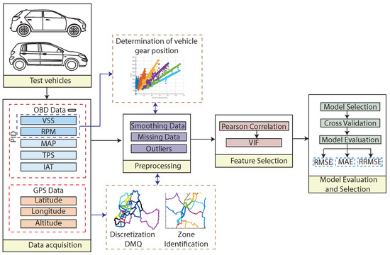
Figure 1.
Methodological workflow for modeling vehicle fuel efficiency under real driving conditions.
2.1. Study Area
Quito is the capital of Ecuador, which is composed of 32 urban areas and 33 suburban areas. In addition, the city has an area of approximately 372.39 , which is 40 km long and only 5 km wide [38]. This situation can lead to slow vehicle flow conditions, particularly in the topographical context of an Andean city [14]. Furthermore, there are only two climatic seasons: summer and the rainy season, which occur from December to May [39]. In this study, all urban areas are selected, along with some rural areas that are highly representative in terms of transfers from densely populated areas to points of interest within the city. The segmentation adopted corresponds to the official administrative divisions of Quito, ensuring reproducibility. The selected areas are presented in Table 1 and Figure 2. The profile of every zone is obtained by extracting layers using the QGIS geospatial application. Subsequently, the obtained layers are plotted in Matlab software to identify each zone in the DMQ.

Table 1.
Identification of study areas.
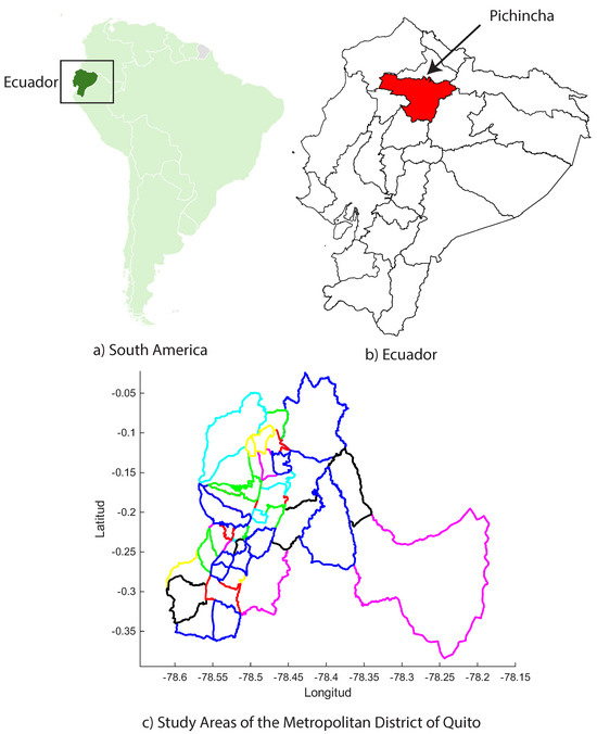
Figure 2.
Considered areas of the Metropolitan District of Quito.
The present study focuses on the DMQ, which is a high-altitude urban area with a specific topographical variability. Therefore, all results and interpretations should be considered local in scope and not generalized to other urban settings without further validation. Nonetheless, the proposed methodology could be adapted to other cities by recalibrating the zoning approach using geographic information in the new model.
2.2. Test Vehicles
Vehicle information data are acquired through the OBD using a physical connector present in each automobile. The sensors can be read through the Parameter Identifier Data (PID) under the SAE J1979 standard [40]. These data include information such as engine revolutions per minute (RPM), vehicle speed (VSS), intake manifold pressure (MAP), throttle pedal position (TPS) and intake air temperature (IAT) [41]. Additional geopositioning information, such as latitude, longitude, and altitude, is taken via a smartphone application that simultaneously records the data. All information on vehicles, including GPS trajectories used in this study, was anonymized prior to preprocessing the data. Moreover, personal information such as driver’s identity, vehicle license number, and location from work or home was removed.
This academic paper focuses on passenger automobiles because they are the second-largest group of vehicles, accounting for 27.86% of the total registered vehicles in Ecuador, after motorcycles, which account for 28.35% [42]. To ensure a diverse sample, eight vehicles are selected with different engine displacements, standard emissions and model years. The chosen vehicles are commonly used in Ecuador; for instance, the Chevrolet Aveo was a best-selling vehicle between 2009 and 2019 [43]. The classification by engine displacements in vehicles for Ecuador according to Normative Technical Ecuadorian (NTE) 2656 is as follows: under 1000 , 1000–1600 , 1600–2000 , and over 2000 [44]. The median engine displacement, according to the Internal Revenue Service (SRI), is 1500 , which is compatible with selected vehicles [11]. The Euro 3 standard was implemented in 2017 for new vehicles in the country, which means that Ecuadorian distribution is older [45]. Overall, while the number of vehicles is limited, the selection strategy captures a realistic cross-section of the current urban fleet in Ecuador. Table 2 shows the vehicles used for this work, where the vehicle manufacturer, engine displacement and emission standard are indicated.
Table 2.
List of vehicles.
The vehicles used in this experimental campaign were driven under typical traffic conditions without prior driver instructions. All routes were driven between 6:00 a.m. and 7:00 p.m. on weekdays and were conducted in dry weather conditions. Data were collected from March 2023 to January 2024, excluding periods with rainy conditions. This period was selected because traffic is heavier during the winter season, and vehicles traveling on the road at low velocities did not cover the entire range of speeds. Altitudes range from 2600 masl in valley areas to 3200 masl, covering altitudes in both the south and north of the DMQ. The fuel consumption calculation for each vehicle was performed using the ideal gas equation, which has been proven to be efficient in [46,47,48]. Figure 3 shows the fuel consumption of the vehicles reported in this study as a function of speed, identifying high consumption values at low speeds due to the energy required to move the vehicle mass from a complete stop in urban traffic. Afterwards, a stabilization phase of fuel consumption at an intermediate velocity between 50 and 80 km/h is followed by a reduction at velocities higher than 80 km/h due to the aerodynamic resistance that the vehicles must overcome as they move through the air.
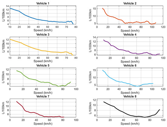
Figure 3.
Velocity vs. fuel consumption.
2.3. Data Preprocessing
The information is acquired through the OBD port of the vehicles at a frequency of 1 Hz. In the first stage, the signals are smoothed by a 5 s centered moving window filter. The altitude parameter is processed with a Savitzky–Golay filter, demonstrating high efficiency for smoothing during changes of slope on the road [30]. Then, outliers are replaced by interpolation using the interquartile range (IQR) method with a factor of 1.5. The gear is selected using decision trees, as all vehicles in the study are equipped with manual transmissions and do not include sensors to detect gear position. It is known that the gearbox and engine exhibit a linear relationship, so the use of the relation allows for the discretization of the activated gear [49].
To identify when a vehicle circulates through a geographic area, the inpolygon function in Matlab is used. Polygons are defined by latitude and longitude, and identifiers between 1 and 35 are assigned according to the position of the GPS coordinates. Subsequently, the variables are standardized to have a mean of zero and a standard deviation of one. Again, an outlier verification stage is performed with those values that present a residual greater than 3. Additionally, a model partition is created using 80% of the data for training and the remaining 20% for testing. Finally, the problem is modeled using the Gamma regression model with a logarithmic link. The predicted fuel efficiency is verified with the RMSE, MAE, and RRMSE metric.
2.4. Calculation of Predictors
Several parameters allow characterizing road driving by describing the dynamic conditions of the vehicle. Acceleration is defined as the rate of change of velocity over time. Its calculation procedure is presented in Equation (1).
A parameter that relates vehicle power to vehicle mass is the VSP, which can also be interpreted as the forces opposing vehicle motion, such as rolling resistance, inertial, aerodynamic, and slope forces, multiplied by speed and divided by vehicle mass, as expressed in Equation (2) [50].
In the literature, it is common to use the simplification shown in Equation (3) described in terms of velocity (v) and acceleration (a) [51,52].
Sometimes, the isolated VSP information is insufficient to describe the driving style or operating conditions of the vehicle; therefore, the International Vehicle Emissions Model (IVE) methodology is used to discretize the VSP information [53,54]. The IVE model introduces the concept of engine stress (ES), which describes the engine load applied at an instant of time. In Equation (4), the term describes the motor speed and is a moving average window that considers past VSP events from second to .
Figure 4 shows the VSP distribution for each vehicle, with the data organized into 60 bins, which are further subdivided into three bands. The first one represents low engine stress, the second represents moderate stress, and the final one represents high engine stress. As can be seen, most of the vehicles fall within the VSP range of to 5 kW/ton, which can be described as predominantly city driving with low engine load, which is characteristic of dense traffic with frequent stops. In addition, the distributions are mostly around zero, identifying a low-load scenario, which reaffirms that the trips were performed in urban areas of the DMQ. Vehicle 5 in this study is the only one that shows an activation of the bins in low and medium load zones, suggesting a higher engine effort.
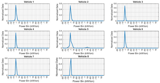
Figure 4.
VSP histogram for each vehicle.
Most of the information that characterizes driving style is described in terms of speed and acceleration. Relative Positive Acceleration (RPA) is a term used to describe a driving style in various road conditions. It considers the variation of speed and acceleration concerning distance in its positive part. In urban areas, can be interpreted as timid driving, while values greater than 0.2 are considered aggressive [32]. Its calculation procedure is shown in Equation (5).
The product of the instantaneous velocity multiplied by the acceleration (VA[95]) is represented in Equation (6). For this parameter, the 95th percentile of the information is estimated by considering only accelerations greater than [55].
2.5. Predictor Selection
To model the study problem, it is necessary to select the variables that provide the most relevant information, considering FE as the response variable. Figure 5 shows the Pearson correlation where vehicle speed (VSS), speed per acceleration (VA[95]), acceleration (A), and engine speed (RPM) have correlations with some degree of importance. The statistical significance of each correlation coefficient was evaluated using a significance level of , confirming that all reported correlations are significantly different from zero (p-value < 0.05). The variable VSP remains in the model despite its low correlation because it may describe possible quadratic interactions. Additionally, the slope describes the potential energy of the vehicle when ascending or descending the roadway, which is related to the study zones.
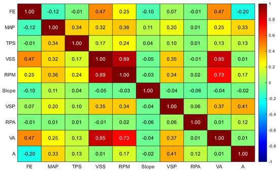
Figure 5.
Pearson correlation plot.
Moreover, to avoid effects related to collinearity between variables, the variance inflation factor (VIF) is calculated, as shown in Table 3. Variables with a VIF lower than five are considered independent. Predictors with values between 5 and 10 should be considered for inclusion in the model. Variables greater than 10 could be removed from the model. It is worth mentioning that the variable RPM was removed because it presented collinearity with VSS. In addition, the variable gear is calculated through the linear relation between VSS and RPM. To verify the impact of this decision, the model was tested both with and without RPM. The inclusion of RPM did not result in a meaningful improvement in performance metrics, suggesting that other variables sufficiently capture the underlying physical dynamics. To assess the model’s stability, the coefficient of variation was calculated for key predictors, yielding the following results: TPS = 3.06%, VSS = 0.61%, and slope = 3.66%. These low values suggest minimal variability and consistent contributions of these variables to the model.
Table 3.
Variance inflation factor.
2.6. Model Selection and Justification
FE is always a positive value; the variable is continuous and, in general, asymmetric. There are several methods to estimate fuel consumption. In [56], a logarithmic transformation is used to predict the relation between the mass of the vehicle and FE due to the identification of nonlinear effects. The Gamma regression model with a logarithmic link offers direct interpretability and effectively handles heteroscedasticity. Although machine learning techniques such as SVM, Random Forest, and ANN demonstrate high prediction accuracy, their interpretability is limited [57]. To sum up, the Gamma model provides coefficients that quantify the effects of explanatory variables, requires minimal hyperparameter tuning to avoid overfitting, and has theoretical consistency. In contrast, algorithms such as Random Forest often require model hybridization to achieve stability, which complicates scalability [58].
3. Results
3.1. Fuel Consumption Distribution by Speed and Zone
For the evaluation of speed and average fuel consumption by zone, the Matlab inpolygon function is used to identify when the points of a vehicle in the route are within a zone, outside a zone or on the edge through the data recorded by GPS. Subsequently, the average speed and consumption per zone are estimated, which allows for associating the vehicle’s behavior with the city’s conditions. In Figure 6, it can be visualized how the calculation algorithm detects the route layout and the interchanges between zones.
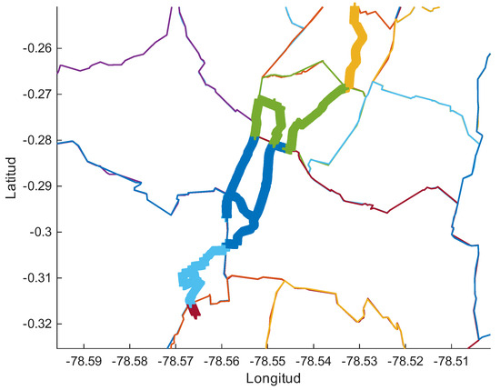
Figure 6.
Distribution of fuel consumption by speed and zone.
In Figure 7 and Figure 8, it can be inferred that there is an efficient circulation in zone 2 for vehicle 5, with a speed of 68.61 km/h, resulting in an FE efficiency of 21.72 km/L. Zones 26 and 28 for vehicle two report speeds of 69.03 km/h and 66.47 km/h, while the consumption values are 19.41 km/L and 16.14 km/L, respectively. This indicates that with speeds between 60 and 70 km/h, typical of arterial roads, the best fuel consumption efficiencies are achieved. Urban operation zones, such as 6 and 8, with speeds of around 20 and 40 km/h, report FE between 5 and 15 km/L. It is also shown that in areas with average speeds below 20 km/h, the consumption can be less than 8 km/L. This is due to the engine displacement, traffic conditions and the driving style of each driver.
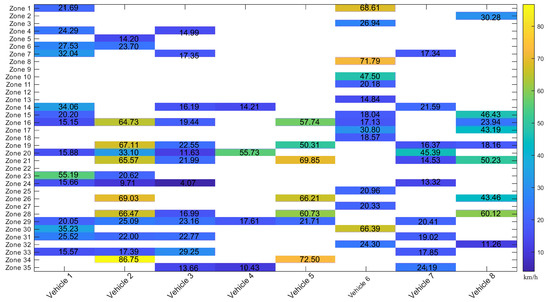
Figure 7.
Heatmap of average speed by study zone.
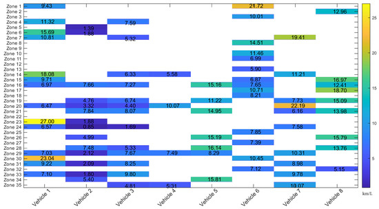
Figure 8.
Heatmap of fuel efficiency by study zone.
3.2. Speed–Acceleration Probability Distribution
The Speed–Acceleration Probability Distribution (SAPD) describes how often a combination of acceleration and speed can occur by discretizing these parameters in bins [59]. In Figure 9, a high frequency of speeds below 15 km/h can be observed, indicating that vehicles were encountered at low speeds most of the time due to urban driving conditions. Furthermore, it is observed that the accelerations are in a band between and , indicating smooth driving without abrupt accelerations or spontaneous stops. Additionally, it is observed that in the regions where the speed exceeds 50 km/h, the accelerations remain around and .
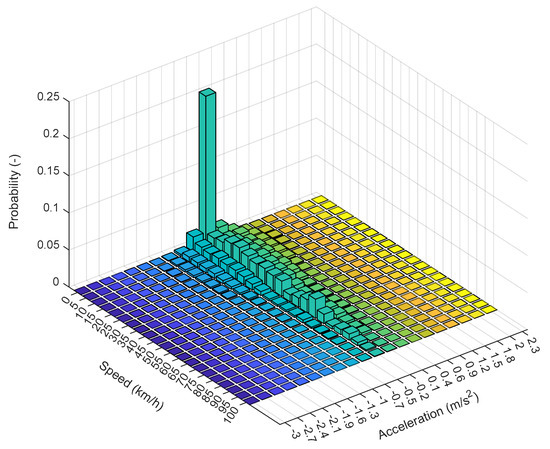
Figure 9.
Speed–Acceleration Probability Distribution (SAPD).
A three-dimensional representation of the specific fuel consumption and VSP is presented in Figure 10. It is observed that the maximum peak represents approximately 28% of the driving conditions, resulting from low engine demands of around kW/ton and 3.9 kW/ton. However, it reports inefficient FE values due to the constant stopping and starting of the vehicle from rest. It is reported that the best fuel consumption efficiencies are found with VSP values close to 3 kW/ton with consumptions between 26 and 30 km/L.
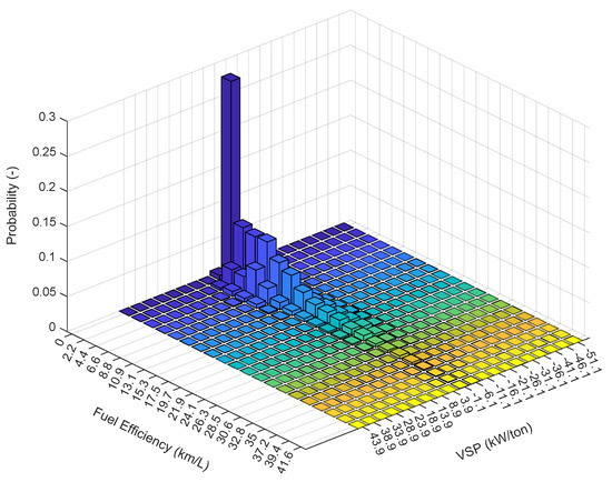
Figure 10.
Fuel efficiency distribution vs. VSP.
A two-dimensional contour representation of FE distribution as a function of VSP is presented in Figure 11. The plot indicates that the most frequent operations fall within the range of to 2 kW/ton with FE reporting between 0 and 2.5 km/L. The zones correspond to low engine load scenarios, which are associated with the deceleration of idling conditions. This graph complements the spatial distribution and density of driving conditions.
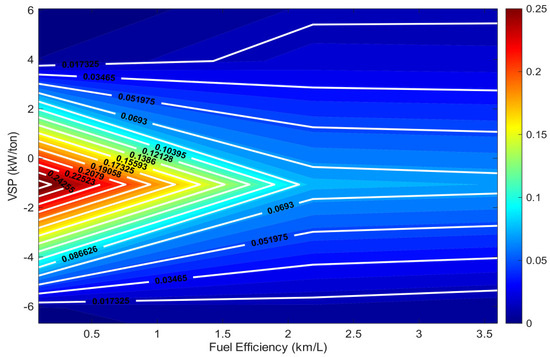
Figure 11.
Contour plot of fuel efficiency distribution as a function of Vehicle-Specific Power.
3.3. Effect of Altitude on Fuel Efficiency
Air pressure changes are correlated with altitude variation, especially in high-altitude areas. A parameter, such as altitude, has an index of correlation of −0.01 and a p-value of 0.003 compared with FE, which indicates the existence of significance but a reduced correlation. In Figure 12, it can be observed how the FE is reduced with the increment in elevation measured as altitude over the sea level. In addition, altitude is a parameter; it does not have a direct interpretation in fuel consumption. In addition, air pressure is a factor that affects engine performance. This factor is estimated from the barometric formula [60]. The relation between FE and pressure yields a correlation of 0.011 and a p-value of 0.001, indicating a weak but statistically significant relationship. For this reason, in this work, the variable slope is used as a predictor because it represents the variation in elevation over a distance. Furthermore, slope and altitude are collinear, reinforcing the decision to use only one of them in the model.
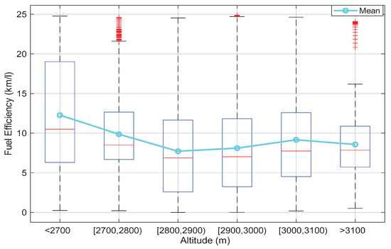
Figure 12.
Boxplot altitude vs. fuel efficiency.
The Analysis of Variance (ANOVA) indicates that group mean differences are statistically significant (p-value < 0.05). In Figure 13, a multiple comparison test with a 95% confidence interval is used to identify groups with differences. For example, group 1, which represents altitudes under 2700 masl, is different from the other groups, as well as group 2 with altitudes between 2700 and 2800 masl. These results suggest that FE is affected by altitude, especially in lower elevations.
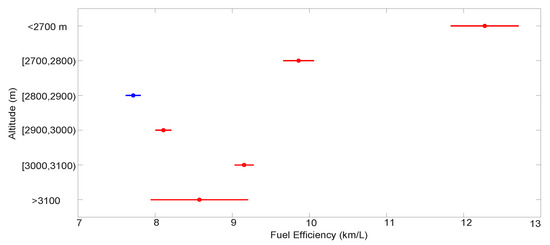
Figure 13.
Multiple comparisons.
3.4. Gamma Regression Model with Logarithmic Link
Fuel efficiency is a strictly positive value with high relative variability, resulting from the constant change in engine operating speeds that is visible when comparing urban versus high-speed driving. A Gamma distribution, which by definition models an increasing variance of the mean of the values, is appropriate for this type of problem. The model used for this work is presented in Equation (7).
where the following apply:
- represents the intercept of the model.
- to are the coefficients of the standardized continuous variables.
- represents the effects by vehicle circulation zone.
- represents the effects by gear selection, where 1 corresponds to the first gear of the transmission.
Table 4 summarizes the model results, with a dispersion value of 0.177 indicating a good model fit, with a low error, which indicates variance-adjusted residuals. At the same time, the F-statistic parameter is high, which supports the effectiveness of the statistical model, along with a p-value of approximately zero. The model accurately represents the physical aspect of the fuel consumption phenomenon; i.e., increasing the speed improves the FE. The positive coefficient of VA[95] indicates that better FE can be achieved through a gradual increase in speeds with constant accelerations. The complete set of estimated coefficients is presented in Table A1. Slope values reduce efficiency, and an increase in acceleration also negatively impacts fuel consumption. The geographical effects on fuel consumption are similar to those shown in Figure 8, where zones 2, 11, 15, 16, and 18 have positive coefficients, indicating zones of efficient consumption. On the other hand, zones 5, 6, 23 and 24 are identified as low efficiency due to vehicle congestion or steep slopes. Regarding gears, it follows that a longer ratio improves efficiency; however, consumption is optimized between third and fifth gear. The model has a Root Mean Square Error (RMSE) of 0.939 over the test set, a relative Root Mean Square Error (RRMSE) of 0.155, a Mean Absolute Error (MAE) of 0.754, and a coefficient of determination ().
Table 4.
Summary of the most relevant coefficients of the linear regression model with Gamma distribution and logarithmic link function.
In Figure 14a, the behavior of the residuals is observed, showing the non-existence of characteristic curves, and most of the residuals tend to be distributed centered at zero. The quantile–quantile plot (QQ-plot) in Figure 14b illustrates how the residuals fit well in the central range while exhibiting a slight curvature in the tails. In Gamma models, the residuals are not expected to be completely normal. Meanwhile, in Figure 14c, we can visualize the histogram of the residuals, which tend to be symmetrically distributed around zero, thus avoiding systematic bias.
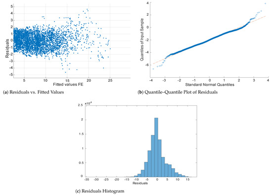
Figure 14.
Graphical residual analysis of the fitted mode.
4. Discussion
In this paper, a Gamma regression model with a logarithmic link was developed to estimate FE in LDVs operating under real driving conditions in the DMQ. The study starts with the selection of predictors that best describe the phenomenon. In this work, variables such as RPA, TPS, and MAP were excluded from the model due to their low correlation with the fuel consumption variable. Although VSP was included in the model because it integrates the instantaneous power used by the vehicle and can indirectly include quadratic terms of other variables, it was found to have no significant effect in the model. The variance inflation method was used to verify that there was no multicollinearity among the predictors. All predictors were below the critical threshold. The highest values correspond to VSS and VA[95] values of 4.103 and 3.806, respectively. The rest of the variables presented VIF values close to one, suggesting relative independence among the predictors. Meanwhile, the variable RPM was removed from the model because it presented a strong dependence relationship with VSS and a VIF of 12.1. In addition, the model is tested with the presence of RPM, finding an RMSE of 0.959, MAE of 0.776, and RRMSE of 0.156, showing no significant improvements with the addition of another variable.
4.1. Model Interpretation and Coefficient Analysis
The Gamma regression model with a logarithmic link is used for this work to predict FE, which is a positive parameter. In general, the model is consistent with vehicular dynamics. For instance, a positive coefficient implies an increase in FE for that variable. The predictor VA[95] with a coefficient of indicates better fuel efficiency if the velocity increases with constant acceleration. Predictors such as slope have a coefficient of . This value implies that an increase in slope will reduce FE because it results in higher engine stress. On the other hand, a downward slope will increase FE. For every unit increase in road gradient, fuel efficiency decreases by approximately 4.3%. This value is similar to the work presented in [61]. An increment of one unit in acceleration reduces FE by 8.1%.
Figure 15 presents a Partial Dependency Plot (PDP) to illustrate the individual contribution to each predictor in the Gamma regression model. As can be shown, an increase in variable VA[95] will improve FE because better fuel economy is associated with reduced engine variability. On the other hand, an increment in acceleration reduces FE, meaning that higher accelerations produce more energy demand. Meanwhile, FE decreases for every increment in the vehicle’s speed because there is a nonlinear relation between aerodynamic drag and velocity. Uphill slopes result in a reduction in FE due to the increased power required by the engine to overcome the additional resistance. An increment in variable VSP improves FE, but the influence of this parameter in the model is tiny.
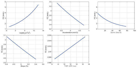
Figure 15.
Partial dependency plot of fuel efficiency.
4.2. Model Performance Analysis and Literature Comparison
Before model training, all continuous variables were standardized with z-score normalization to avoid scale-related distortion. In addition, standardized residuals were calculated to identify outliers. Following the process of outlier removal, the dataset was evaluated using 5-fold cross-validation to ensure robust and representative performance metrics. In each fold, 80% of the data was used to train the model, and the remaining 20% was used for validation. In order to verify the robustness of the proposed Gamma regression model, a comparative analysis was performed in Matlab using a machine learning approach based on ensemble regression trees. This algorithm is similar to the implementation of XGBoost. After the implementation of fitrensemble, the Gamma regression model achieved a lower RMSE of 0.939 vs. 1.711, a reduction in MAE (0.754 vs. 1.146), and a higher coefficient of determination ( = 0.956 vs. 0.8525). Additionally, the RRMSE was significantly reduced (0.155 vs. 0.2787), confirming that the model proposed in this work is suitable for the estimation of FE in vehicles.
The results obtained for the model demonstrate stability and consistency with vehicle dynamics, but it is necessary to compare with other studies. For example, in the study conducted by Rykala et al. [27], fuel consumption is predicted for a single vehicle using a multiple regression model with the predictors’ slope, engine load, RPM, A, and VSS, yielding an MAE of 1.25. Instead, this study used the Gamma model, which obtained an MAE of 0.757, thereby improving the fuel consumption estimation. In this work, prior to implementing the Gamma model and logarithmic link, models such as linear regression were tested, finding adjustments of and RMSE of 4.66. With Linear Support Vector Machine (SVM) results featuring an and RMSE of 4.859, these options were discarded. It is assumed that the reported differences are due to the inclusion of more study vehicles and geographic zones, which means that the linear models could not efficiently predict consumption. In another work developed by Zeng et al. [62], fuel consumption in LDVs is estimated using information reported by the owners. In their work, several models are analyzed, finding values of for linear regression, for Naive Bayes, and for a Light Gradient Boosting Machine (Light GBM) model, a and an MSE of 1.536 similar to those reported by the Log-Gamma model are obtained. In another work developed by Ashqar et al. [63], the driving style variable is incorporated into the model, initially using a linear regression model to obtain an of 0.511 and an MSE of 0.031. Later, using a Random Forest model, they achieve a fit of and an MSE of 0.003, which better captures the interaction between predictors. When comparing the results with this work, the MSE is lower; however, the Log-Gamma model allows for a direct explanation of each factor and its interaction with others at a reduced computational cost. In a related study, developed in Colombia, a high-altitude country, Díaz et al. [64] present a regression model to estimate fuel consumption after implementing an ecodriving campaign on a freight fleet, yielding values of 0.79 and 0.73 for the baseline and post-campaign periods, respectively. They indicate that significant variables in the study are weight, utilization, ascendant route indicator, excessive RPM use, and percentage outside the green band. The model used in this work has similar explanatory variables to the study, except for RPM and the indicator of fuel efficiency. To compare the results of this study with those of other studies, an approximate coefficient of determination was computed based on the residual sum of squares. The resulting value of 0.95 suggests that our model explains 95% of the variability of FE. Huertas et al. [65] in their study of a fleet of trucks in Colombian corridors found that there is no evidence that specific fuel consumption is greater or increases with altitude, which is similar to the findings reported in this work. Furthermore, fuel consumption is a parameter related to slope and also describes limitations of access to historical georeferenced data on fuel consumption, which is covered in our work. Giraldo et al. [21] studied a fleet of buses powered by diesel fuel in the Mexico City area, operating at an altitude of 2000 masl. Using a multiple linear correlation analysis between fuel consumption and driving characteristic parameters, an adjusted determination coefficient of 0.8 is obtained. They also found that slope grade is an important predictor. In addition, the variable that accounts for the positive kinetic energy per distance traveled is the most representative parameter. Moreover, the VSP parameter is poorly correlated with FE, which yields a similar value compared to this study. Rondon et al. [66] study the variation in fuel consumption and emission in LDVs. This parameter is calculated using the air intake flow from the manifold. They evaluated the effect of VSP using gasoline–ethanol blends in real traffic conditions. This study supports the applicability of VSP in urban settings, but it does not consider altitude-related variables such as air pressure or topographic slope. In contrast, our work expands the scope by incorporating high-altitude factors, which significantly influence engine performance and fuel efficiency. A study by Mardonez et al. [67] in the cities of Paz and Alto found that steep slopes can significantly increase vehicle fuel consumption, as combustion efficiency decreases due to reduced oxygen. This finding increases the importance of integrating topographic characteristics and atmospheric conditions.
4.3. Practical Implications and Applications
The model presented in this work allows the identification of key variables that impact fuel efficiency, such as vehicle speed, acceleration, VA[95], gear usage, and geographic zones. This information is helpful for tasks such as optimizing traffic signals and route planning. For instance, reducing unnecessary accelerations and decelerations is a crucial parameter for limiting fuel consumption. Traffic signals can be adjusted to promote a smoother flow, particularly in critical zones identified by the model. A similar approach to this work is realized by Alshayeb et al. [68], who integrate fuel consumption index, traffic simulation, and the stochastic genetic algorithm to improve sustainability and mobility efficiency. Their study focuses on 13 signalized intersections in Chicago. With the implementation of the solution, they achieve fuel consumption savings of between 8 and 12% under moderate operating conditions. Their results demonstrate the effectiveness of integrating fuel-oriented optimization within traffic signal control strategies. Route planning is another area where the algorithm developed in this paper could improve FE by identifying efficient routes to minimize timing and reduce FE. The route selection not only depends on a schedule but also considers the use of efficient zones. In the work proposed by Ganji et al. [69], a supply chain problem is optimized through scheduling and multi-objective programming, demonstrating that incorporating fuel consumption into operational decisions can lead to improved outcomes. In addition, the presented model for this academic work quantifies dynamic conditions, making it applicable to real-world traffic management strategies. Optimizing traffic signals to reduce stopping time translates into a smoother profile in the speed of vehicles, improving FE. Another practical application is the integration of FE models with traffic data and vehicle connectivity. In work [70], the addition of fuel consumption is presented to evaluate the reduction for an automated vehicle at level 1. The experimental procedure is conducted under real operational conditions to introduce route characteristics, traffic conditions, and driver behavior. The authors of the study mentioned that route and traffic information can achieve fuel savings of 15 to 19%.
4.4. Limitations and Future Research Recommendations
The results of this study offer valuable insights for the development of transportation policies for high-altitude cities such as DMQ. First, identifying zones with low FE highlights the importance of realizing improvements in traffic management. Second, road slope grade is an important variable in FE. Given this condition, it is advisable to consider the use of electric or hybrid mobility in these zones. Third, policymakers should consider integrating geographic and dynamic variables of vehicles for future emission inventories. Finally, this study should be complemented with the inclusion of an extensive database of vehicles monitored in real time to optimize FE under real conditions of driving.
Although the model developed in this work demonstrates high performance with information on vehicles driving in the DMQ, the generalization ability of the model in other Andean cities has not yet been proved. This fact represents a potential limitation of the study. Future research should consider cross-regional validation to test the model in other cities such as La Paz or Bogota.
5. Conclusions
In the present work, a Gamma regression model with a logarithmic link was developed to predict FE for vehicles in a high-altitude city, such as the DMQ, under real conditions, including PID, geoposition, and driving style information. The significant predictors of the model were VSS, RPM, A, and VA[95]. Additionally, the variables slope, gear shift changes, and circulation zone determined through polygon-based detection were integrated into the model. The model has an RMSE of 0.939 over the test set, an RRMSE of 0.155, an MAE of 0.754, and an approximate coefficient of determination () of 0.956, which is significant considering the variability of data obtained under real driving conditions.
The model penalizes critical circulation zones in terms of fuel efficiency. Predictors were selected by Pearson correlation with VIF verification. Additionally, the model assumptions indicate that the residuals are distributed around a center at zero, thereby avoiding systematic bias.
The model employs a dynamic approach, considering variables such as VA[95], VSP, VSS, categorical transmission shift data, and traffic zones. When analyzing the model, it aligns with preliminary data reported in the heat maps, where zones 5, 6, 23, and 24 exhibit constant stops, and zones 2, 11, 15, 16, and 18 are considered free flowing. The VSP parameter adds value information because it describes driving behavior. Moreover, this information is complemented by SAPD, which describes how often a combination of acceleration and speed can occur. In this case, within DMQ, a high density of velocities under 15 km/h is observed. Also, accelerations are between ±1 m/s2, indicating driving without abrupt acceleration typical of urban areas. FE vs. VSP report that the most frequent operation occurs between and 2 kW/ton with values of FE in the range of 0 to 2.5 km/L.
Altitude is a parameter related to air pressure. Although elevation and air pressure have statistical significance with FE, the correlation is weak. Altitude is a parameter in itself, not describing fuel consumption. However, the best performance of FE is achieved with altitudes under 2700 masl with values between 11.9 and 12.8 km/L after a multiple comparison test. The analysis supports the inclusion of slope as a predictor because it captures changes in elevation over a distance.
The Gamma regression model with a logarithmic link function was used to predict FE, which is a strictly positive factor. The model has consistency with vehicular dynamics, allowing physical interpretation between input variables and the response variable. Variables such as VA[95] exhibit a positive coefficient, indicating that fuel consumption could be improved with constant acceleration and increasing speed. Slope gradient is a predictor with a negative coefficient, which implies that an increment of one unit in this variable will decrease FE by approximately 4.3%.
While the results are exploratory and developed in the context of the DMQ, they provide valuable insights into the relationship between driving behavior and topographic characteristics for predicting FE. Although the sample may not constitute a statistically representative sample of all vehicles, it captures the diversity of real driving patterns in an urban Andean city.
In future work, we intend to integrate a larger and more diverse dataset to enhance the robustness and generalizability of the proposed model. This approach can serve as a tool for decision making in the DMQ. Areas of low vehicle efficiency in the city can be detected not only by measuring traffic times but also in terms of energy. Although vehicles powered by internal combustion engines represent the majority of the population, alternative technologies, such as diesel engines, electric vehicles, and hybrids, should be incorporated. Their differences in traffic conditions should be reported.
Author Contributions
Conceptualization, P.A.M.-C.; Methodology, J.J.M.-C.; Software, P.A.M.-C.; Validation, J.J.M.-C.; Investigation, J.T.-P.; Data curation, P.A.M.-C.; Writing—original draft, J.J.M.-C. and P.A.M.-C.; Writing—review and editing, P.A.M.-C. All authors have read and agreed to the published version of the manuscript.
Funding
Grupo de Ingeniería Automotriz, Movilidad y Transporte (GiAUTO), Carrera de Ingeniería Automotriz-Campus Sur, Universidad Politécnica Salesiana, Quito 170702, Ecuador.
Institutional Review Board Statement
Not applicable.
Informed Consent Statement
Not applicable.
Data Availability Statement
The original contributions presented in the study are included in the article; further inquiries can be directed to the corresponding author.
Acknowledgments
To Universidad Politécnica Salesiana, Ecuador for funding the research project 083-05-2025-01-08: “Estimación de Factores de Emisión en Vehículos Ligeros a partir de Pruebas en Condiciones Reales de Circulación”.
Conflicts of Interest
The author declares no conflicts of interest.
Abbreviations
The following abbreviations are used in this manuscript:
| RMSE | Root Mean Square Error |
| RRMSE | Relative Root Mean Square Error |
| VA[95] | 95th percentile of positive acceleration multiplied by vehicle speed |
| MAE | Mean Absolute Error |
| Carbon Dioxide | |
| LDV | Light Duty Vehicle |
| CO | Carbon Monoxide |
| INEC | National Institute of Statistics and Censuses |
| DMQ | Metropolitan District of Quito |
| AEADE | Association of Automotive Companies of Ecuador |
| NTE | Normative Technical Ecuadorian |
| SRI | Internal Revenue Service |
| CAN | Controller Area Network |
| MRAE | Mean Relative Absolute Error |
| Nitrogen Oxides | |
| VSP | Vehicle-Specific Power |
| IVE | International Vehicle Emissions Model |
| OBD | On-Board Diagnostics |
| PID | Paramemeter Identifier Data |
| VSS | Vehicle Speed |
| ECT | Engine Coolant Temperature |
| IAT | Air Intake Temperature |
| MAP | Manifold Absolute Pressure |
| ANOVA | Analysis of Variance |
| IQR | Interquartile Range |
| RPA | Relative Positive Aceleration |
| A | Aceleration |
| VIF | Variance Inflation Factor |
| SAPD | Speed-Acceleration Probability Distribution |
| Q-Q plot | Quantile-quantile plot |
| PDP | Partial Dependency Plot |
| SVM | Linear Support Vector Machine |
Appendix A
Table A1 presents the estimated coefficients of the generalized linear model with a Gamma distribution and a logarithmic link function.
Table A1.
Estimated coefficients of the generalized linear regression model with a Gamma distribution and a logarithmic link function.
Table A1.
Estimated coefficients of the generalized linear regression model with a Gamma distribution and a logarithmic link function.
| Variable | Estimate | SE | tStat | p-Value | Variable | Estimate | SE | tStat | p-Value |
|---|---|---|---|---|---|---|---|---|---|
| (Intercept) | −0.243 | 0.012 | −19.949 | VA | 0.330 | 0.008 | 43.273 | ≈0 | |
| Aceleration | −0.085 | 0.003 | −27.559 | VSS | −0.533 | 0.009 | −57.133 | ≈0 | |
| Slope | −0.044 | 0.002 | −21.784 | VSP | 0.001 | 0.004 | 0.176 | 0.860 | |
| Zone 1 | 0.168 | 0.159 | 1.051 | 0.293 | Zone 2 | 0.345 | 0.025 | 13.603 | |
| Zone 3 | 0.288 | 0.211 | 1.365 | 0.172 | Zone 4 | −0.086 | 0.028 | −3.054 | 0.002 |
| Zone 5 | −1.369 | 0.018 | −74.184 | ≈0 | Zone 6 | −1.299 | 0.023 | −55.348 | ≈0 |
| Zone 7 | −0.271 | 0.037 | −7.398 | Zone 8 | 0.364 | 0.244 | 1.497 | 0.135 | |
| Zone 10 | 0.412 | 0.211 | 1.951 | 0.051 | Zone 11 | 0.676 | 0.078 | 8.717 | |
| Zone 13 | 0.130 | 0.046 | 2.823 | 0.005 | Zone 14 | −0.055 | 0.014 | −3.892 | |
| Zone 15 | 0.243 | 0.022 | 10.876 | Zone 16 | 0.250 | 0.017 | 14.719 | ||
| Zone 17 | 0.232 | 0.057 | 4.059 | Zone 18 | 0.198 | 0.029 | 6.784 | ||
| Zone 19 | −0.135 | 0.017 | −7.891 | Zone 20 | −0.265 | 0.020 | −13.392 | ||
| Zone 21 | −0.173 | 0.018 | −9.635 | Zone 23 | −1.325 | 0.017 | −76.606 | ≈0 | |
| Zone 24 | −0.443 | 0.014 | −32.633 | Zone 25 | 0.129 | 0.070 | 1.844 | 0.065 | |
| Zone 26 | −0.314 | 0.031 | −10.132 | Zone 27 | 0.197 | 0.019 | 10.099 | ||
| Zone 28 | −0.156 | 0.016 | −10.050 | Zone 29 | −0.231 | 0.012 | −19.619 | ||
| Zone 30 | −0.016 | 0.064 | −0.258 | 0.796 | Zone 31 | −0.333 | 0.015 | −22.583 | |
| Zone 32 | 0.293 | 0.050 | 5.829 | Zone 33 | −0.278 | 0.013 | −21.233 | ||
| Zone 34 | −0.436 | 0.018 | −24.794 | Zone 35 | −0.004 | 0.016 | −0.260 | 0.795 | |
| Gear 1 | 1.516 | 0.009 | 177.200 | ≈0 | Gear 2 | 2.271 | 0.010 | 222.250 | ≈0 |
| Gear 3 | 2.796 | 0.014 | 198.970 | ≈0 | Gear 4 | 3.031 | 0.019 | 161.300 | ≈0 |
| Gear 5 | 3.274 | 0.026 | 128.200 | ≈0 | Gear 6 | 3.285 | 0.045 | 73.718 | ≈0 |
References
- Páez, C.F.T.; Guayanlema, V.; Mera, A.G.C. Estimation of energy consumption due to the elimination of an environmental tax in Ecuador. Energy Sustain. Dev. 2022, 66, 92–100. [Google Scholar] [CrossRef]
- Yang, Z.; Bandivadekar, A. Light-Duty Vehicle Greenhouse Gas and Fuel Economy Standards; International Council on Clean Transportation: Washington, DC, USA, 2017; Available online: http://theicct.org/sites/default/files/publications/2017-Global-LDV-Standards-Update_ICCT-Report_23062017_vF.pdf (accessed on 7 July 2025).
- Buenaño, E.; Padilla, E.; Alcántara, V. Relevant sectors in CO2 emissions in Ecuador and implications for mitigation policies. Energy Policy 2021, 158, 112551. [Google Scholar] [CrossRef]
- Molina, P.; Parra, R.; Grijalva, F. Analysis of Driving Style and Its Influence on Fuel Consumption for the City of Quito, Ecuador: A Data-Driven Study. In Proceedings of the International Conference on Applied Technologies, Samborondon, Ecuador, 22–24 November 2023; Springer: Cham, Switzerland, 2023; pp. 247–261. [Google Scholar]
- Viteri, R.; Borge, R.; Paredes, M.; Pérez, M.A. A high resolution vehicular emissions inventory for Ecuador using the IVE modelling system. Chemosphere 2023, 315, 137634. [Google Scholar] [CrossRef] [PubMed]
- INEC. Anuario de Estadísticas de Transporte 2021; Instituto Nacional de Estadística y Censos (INEC): Abuja, Nigeria, 2021; Available online: https://www.ecuadorencifras.gob.ec/documentos/web-inec/Estadisticas_Economicas/Estadistica%20de%20Transporte/ESTRA_2021/2021_ESTRA_PPT.pdf (accessed on 7 July 2025).
- AEADE. Anuario 2023 de Asociación de Empresas Automorices del Ecuador; Asociación Ecuatoriana Automotriz (AEADE): Quito, Ecuador, 2023; Available online: https://www.aeade.net/wp-content/uploads/2024/03/AEADE-2023.pdf (accessed on 7 July 2025).
- Guayanlema, V.; Espinoza, S.; Ramirez, A.; Núñez, A. Trends and mitigation options of greenhouse gas emissions from the road transport sector in ecuador. WIT Trans. Ecol. Environ. 2014, 191, 933–941. [Google Scholar] [CrossRef]
- Campoverde, P.M.; Benavides, K.; Montenegro, F.; Molina, J. Fuel Consumption Analysis of an MPI Engine by Varying Fuel Type, Fuel Filtering, and Air Filter Employing a Full-factor Analysis. In Proceedings of the 2023 IEEE Seventh Ecuador Technical Chapters Meeting (ECTM), Ambato, Ecuador, 10–13 October 2023; IEEE: New York, NY, USA, 2023; pp. 1–6. [Google Scholar]
- Chandi, G.M.; Muñoz, M.; Cárdenas, L.M.F.; Espín, M.R. Estudio de la variación del grado de octanaje mediante mezclas de gasolinas extra, súper y aditivo mejorador de octanaje en Ecuador. Eur. Public Soc. Innov. Rev. 2025, 10, 1–18. [Google Scholar] [CrossRef]
- Terneus Páez, C.F.; Cabrera Mera, A.G.; Grandes Villamarín, R.D. Impact Analysis of Migration from Súper Gasoline to Others of Lower Octane Number in Ecuador. In Proceedings of the International Conference on Intelligent Information Technology, Hanoi, Vietnam, 19–22 February 2020; Springer: Cham, Switzerland, 2020; pp. 95–108. [Google Scholar]
- INRIX. The 2022 Global Traffic Scorecard. 2022. Available online: https://inrix.com/scorecard/#form-download-the-full-report (accessed on 31 May 2023).
- Informe de Movilidad de Quito Cómo Vamos. 2022. Available online: https://quitocomovamos.org/wp-content/uploads/2022/12/07Factsheet_Movilidad2022.pdf (accessed on 28 February 2025).
- González-Rodríguez, M.S.; Clairand, J.M.; Soto-Espinosa, K.; Jaramillo-Fuelantala, J.; Escrivá-Escrivá, G. Urban traffic flow mapping of an andean capital: Quito, ecuador. IEEE Access 2020, 8, 195459–195471. [Google Scholar] [CrossRef]
- Patiño-Aroca, M.; Hernández-Paredes, T.; Panchana-López, C.; Borge, R. Source apportionment of ambient pollution levels in Guayaquil, Ecuador. Heliyon 2024, 10, e31613. [Google Scholar] [CrossRef]
- Feng, H.; Wang, X.; Jia, Q.; Zhu, M. A novel spatial disaggregation model of vehicle emission inventory. Urban Clim. 2024, 55, 101947. [Google Scholar] [CrossRef]
- Van Mierlo, J.; Maggetto, G.; Van de Burgwal, E.; Gense, R. Driving style and traffic measures-influence on vehicle emissions and fuel consumption. Proc. Inst. Mech. Eng. Part D J. Automob. Eng. 2004, 218, 43–50. [Google Scholar] [CrossRef]
- Huang, C.; Lou, D.; Hu, Z.; Feng, Q.; Chen, Y.; Chen, C.; Tan, P.; Yao, D. A PEMS study of the emissions of gaseous pollutants and ultrafine particles from gasoline-and diesel-fueled vehicles. Atmos. Environ. 2013, 77, 703–710. [Google Scholar] [CrossRef]
- Gallus, J.; Kirchner, U.; Vogt, R.; Benter, T. Impact of driving style and road grade on gaseous exhaust emissions of passenger vehicles measured by a Portable Emission Measurement System (PEMS). Transp. Res. Part D Transp. Environ. 2017, 52, 215–226. [Google Scholar] [CrossRef]
- Park, J.; Seo, J.; Park, S. Development of vehicle emission rates based on vehicle-specific power and velocity. Sci. Total. Environ. 2023, 857, 159622. [Google Scholar] [CrossRef]
- Giraldo, M.; Huertas, J.I. Real emissions, driving patterns and fuel consumption of in-use diesel buses operating at high altitude. Transp. Res. Part D Transp. Environ. 2019, 77, 21–36. [Google Scholar] [CrossRef]
- Ren, Y.; Yu, W.; Hao, L.; Ge, Y. Effects of altitude on light gasoline vehicles: Fuel consumption and Air pollution. Atmos. Pollut. Res. 2025, 2025, 102652. [Google Scholar] [CrossRef]
- Song, G.; Yu, L. Estimation of fuel efficiency of road traffic by characterization of vehicle-specific power and speed based on floating car data. Transp. Res. Rec. 2009, 2139, 11–20. [Google Scholar] [CrossRef]
- Hao, L.; Wang, C.; Yin, H.; Hao, C.; Wang, H.; Tan, J.; Wang, X.; Ge, Y. Model-based estimation of light-duty vehicle fuel economy at high altitude. Adv. Mech. Eng. 2019, 11, 1687814019886252. [Google Scholar] [CrossRef]
- Duarte, G.O.; Gonçalves, G.A.; Baptista, P.C.; Farias, T.L. Establishing bonds between vehicle certification data and real-world vehicle fuel consumption–a vehicle specific power approach. Energy Convers. Manag. 2015, 92, 251–265. [Google Scholar] [CrossRef]
- Wu, T.; Han, X.; Zheng, M.M.; Ou, X.; Sun, H.; Zhang, X. Impact factors of the real-world fuel consumption rate of light duty vehicles in China. Energy 2020, 190, 116388. [Google Scholar] [CrossRef]
- Rykała, M.; Grzelak, M.; Rykała, Ł.; Voicu, D.; Stoica, R.M. Modeling Vehicle Fuel Consumption Using a Low-Cost OBD-II Interface. Energies 2023, 16, 7266. [Google Scholar] [CrossRef]
- Sofwan, N.M.; Latif, M.T. Characteristics of the real-driving emissions from gasoline passenger vehicles in the Kuala Lumpur urban environment. Atmos. Pollut. Res. 2021, 12, 306–315. [Google Scholar] [CrossRef]
- Zhou, M.; Jin, H.; Wang, W. A review of vehicle fuel consumption models to evaluate eco-driving and eco-routing. Transp. Res. Part Transp. Environ. 2016, 49, 203–218. [Google Scholar] [CrossRef]
- Moradi, E.; Miranda-Moreno, L. Vehicular fuel consumption estimation using real-world measures through cascaded machine learning modeling. Transp. Res. Part Transp. Environ. 2020, 88, 102576. [Google Scholar] [CrossRef]
- Zhou, X.; Huang, J.; Lv, W.; Li, D. Fuel consumption estimates based on driving pattern recognition. In Proceedings of the 2013 IEEE International Conference on Green Computing and Communications and IEEE Internet of Things and IEEE Cyber, Physical and Social Computing, Beijing, China, 20–23 August 2013; IEEE: New York, NY, USA, 2013; pp. 496–503. [Google Scholar]
- Shahariar, G.H.; Bodisco, T.A.; Zare, A.; Sajjad, M.; Jahirul, M.I.; Van, T.C.; Bartlett, H.; Ristovski, Z.; Brown, R.J. Impact of driving style and traffic condition on emissions and fuel consumption during real-world transient operation. Fuel 2022, 319, 123874. [Google Scholar] [CrossRef]
- Rosero, F.; Rosero, C.X.; Segovia, C. Towards Simpler Approaches for Assessing Fuel Efficiency and CO2 Emissions of Vehicle Engines in Real Traffic Conditions Using On-Board Diagnostic Data. Energies 2024, 17, 4814. [Google Scholar] [CrossRef]
- Almachi, J.C.; Saguay, J.; Anrango, E.; Cando, E.; Reina, S. Clustering-Based Urban Driving Cycle Generation: A Data-Driven Approach for Traffic Analysis and Sustainable Mobility Applications in Ecuador. Sustainability 2025, 17, 3353. [Google Scholar] [CrossRef]
- Montúfar Paz, P.A.; Cuisano, J.C. Development and Validation of a Methodology for Predicting Fuel Consumption and Emissions Generated by Light Vehicles Based on Clustering of Instantaneous and Cumulative Vehicle Power. Vehicles 2025, 7, 16. [Google Scholar] [CrossRef]
- Romero, C.A.; Correa, P.; Ariza Echeverri, E.A.; Vergara, D. Strategies for reducing automobile fuel consumption. Appl. Sci. 2024, 14, 910. [Google Scholar] [CrossRef]
- Patil, M.; Moon, J.; Hanif, A.; Ahmed, Q. Fuel Consumption Estimation Using Spatio-Temporal Modeling and Traffic Flow Predictions: A Comparative Analysis. Technical Report, SAE Technical Paper. 2025. Available online: https://saemobilus.sae.org/papers/fuel-consumption-estimation-using-spatio-temporal-modeling-traffic-flow-predictions-a-comparative-analysis-2025-01-8101 (accessed on 7 July 2025).
- Bravo-Moncayo, L.; Chávez, M.; Puyana, V.; Lucio-Naranjo, J.; Garzón, C.; Pavón-García, I. A cost-effective approach to the evaluation of traffic noise exposure in the city of Quito, Ecuador. Case Stud. Transp. Policy 2019, 7, 128–137. [Google Scholar] [CrossRef]
- Valencia, V.H.; Levin, G.; Ketzel, M. Downscaling global anthropogenic emissions for high-resolution urban air quality studies. Atmos. Pollut. Res. 2022, 13, 101516. [Google Scholar] [CrossRef]
- Uvarov, K.; Ponomarev, A. Driver identification with OBD-II public data. In Proceedings of the 2021 28th Conference of Open Innovations Association (FRUCT), Moscow, Russia, 27–29 January 2021; IEEE: New York, NY, USA, 2021; pp. 495–501. [Google Scholar]
- Lattanzi, E.; Freschi, V. Machine learning techniques to identify unsafe driving behavior by means of in-vehicle sensor data. Expert Syst. Appl. 2021, 176, 114818. [Google Scholar] [CrossRef]
- Instituto Nacional de Estadística y Censos (INEC). Presentación de resultados de las Estadísticas de Transporte (ESTRA) correspondientes al año 2023. In Anuario de Estadísticas de Transporte 2023; Instituto Nacional de Estadística y Censos (INEC): Quito, Ecuador, 2024. [Google Scholar]
- Mera, Z.; Rosero, F.; Rosero, R.; Tapia, F.; Ibarra-Espinosa, S. Effect of idling and power demand on fuel consumption and CO2 emissions from taxis. Enfoque UTE 2025, 16, 1–9. [Google Scholar] [CrossRef]
- Instituto Ecuatoriano de Normalización (INEN). NTE INEN 2656: Clasificación Vehicular. Norma Técnica Ecuatoriana. 2016. Available online: https://www.normalizacion.gob.ec (accessed on 7 July 2025).
- Ibarra-Espinosa, S.; Mera, Z.; Rosero, R.; Díaz, M.V. Spatial and temporal characterization of vehicular emissions in Ecuador using VEIN. In Proceedings of the 2021 Congreso Colombiano y Conferencia Internacional de Calidad de Aire y Salud Pública (CASAP), Bogota, Colombia, 3–5 November 2021; IEEE: New York, NY, USA, 2021; pp. 1–5. [Google Scholar]
- Meseguer, J.E.; Calafate, C.T.; Cano, J.C.; Manzoni, P. Assessing the impact of driving behavior on instantaneous fuel consumption. In Proceedings of the 2015 12th Annual IEEE Consumer Communications and Networking Conference (CCNC), Las Vegas, NV, USA, 9–12 January 2015; IEEE: New York, NY, USA, 2015; pp. 443–448. [Google Scholar]
- Andrade, P.; Silva, I.; Silva, M.; Flores, T.; Cassiano, J.; Costa, D.G. A tinyml soft-sensor approach for low-cost detection and monitoring of vehicular emissions. Sensors 2022, 22, 3838. [Google Scholar] [CrossRef] [PubMed]
- Silva, M.; Signoretti, G.; Silva, I.; Ferrari, P. Performance evaluation of a vehicular edge device for customer feedback in Industry 4.0. ACTA IMEKO 2020, 9, 88. [Google Scholar] [CrossRef]
- Batallas, M.; Molina, P. Developing a Methodology to Reduce Fuel Consumption and Classify Driving Styles for a Fleet of Vehicles. In Proceedings of the International Conference on Science, Technology and Innovation for Society, Guayaquil, Ecuador, 18–19 July 2024; Springer: Cham, Switzerland, 2024; pp. 185–194. [Google Scholar]
- Wang, W.; Bie, J.; Yusuf, A.; Liu, Y.; Wang, X.; Wang, C.; Chen, G.Z.; Li, J.; Ji, D.; Xiao, H.; et al. A new vehicle specific power method based on internally observable variables: Application to CO2 emission assessment for a hybrid electric vehicle. Energy Convers. Manag. 2023, 286, 117050. [Google Scholar] [CrossRef]
- Jimenez-Palacios, J.L. Understanding and Quantifying Motor Vehicle Emissions with Vehicle Specific Power and TILDAS Remote Sensing. Ph.D. Thesis, Massachusetts Institute of Technology, Cambridge, MA, USA, 1998. [Google Scholar]
- Ng, E.C.; Huang, Y.; Hong, G.; Zhou, J.L.; Surawski, N.C. Reducing vehicle fuel consumption and exhaust emissions from the application of a green-safety device under real driving. Sci. Total. Environ. 2021, 793, 148602. [Google Scholar] [CrossRef]
- International Sustainable Systems Research Center (ISSRC). IVE Model Users Manual Version 2.0; International Sustainable Systems Research Center: Los Angeles, CA, USA, 2008; Available online: http://issrc.org/ive/downloads/manuals/UsersManual.pdf (accessed on 7 July 2025).
- Zhao, H.; Mu, L.; Li, Y.; Qiu, J.; Sun, C.; Liu, X. Unregulated emissions from natural gas taxi based on IVE model. Atmosphere 2021, 12, 478. [Google Scholar] [CrossRef]
- Al-Wreikat, Y.; Serrano, C.; Sodré, J.R. Driving behaviour and trip condition effects on the energy consumption of an electric vehicle under real-world driving. Appl. Energy 2021, 297, 117096. [Google Scholar] [CrossRef]
- Tolouei, R.; Titheridge, H. Vehicle mass as a determinant of fuel consumption and secondary safety performance. Transp. Res. Part D Transp. Environ. 2009, 14, 385–399. [Google Scholar] [CrossRef]
- Perrotta, F.; Parry, T.; Neves, L.C. Application of machine learning for fuel consumption modelling of trucks. In Proceedings of the 2017 IEEE International Conference on Big Data (Big Data), Boston, MA, USA, 11–14 December 2017; IEEE: New York, NY, USA, 2017; pp. 3810–3815. [Google Scholar]
- Hassan, M.A.; Salem, H.; Bailek, N.; Kisi, O. Random forest ensemble-based predictions of on-road vehicular emissions and fuel consumption in developing urban areas. Sustainability 2023, 15, 1503. [Google Scholar] [CrossRef]
- Huertas, J.I.; Giraldo, M.; Quirama, L.F.; Díaz, J. Driving cycles based on fuel consumption. Energies 2018, 11, 3064. [Google Scholar] [CrossRef]
- D’yachenko, A.T. Study of the Barometric Formula for the Earth’s Atmosphere. Int. J. Appl. Phys. 2025, 10, 10–13. [Google Scholar]
- Tang, G.; Liu, D.; Liu, J.; Deng, X. Research on the Correlation Mechanism Between Complex Slopes of Mountain City Roads and the Real Driving Emission of Heavy-Duty Diesel Vehicles. Sustainability 2025, 17, 554. [Google Scholar] [CrossRef]
- Zeng, I.Y.; Tan, S.; Xiong, J.; Ding, X.; Li, Y.; Wu, T. Estimation of real-world fuel consumption rate of light-duty vehicles based on the records reported by vehicle owners. Energies 2021, 14, 7915. [Google Scholar] [CrossRef]
- Ashqar, H.I.; Obaid, M.; Jaber, A.; Ashqar, R.; Khanfar, N.O.; Elhenawy, M. Incorporating driving behavior into vehicle fuel consumption prediction: Methodology development and testing. Discov. Sustain. 2024, 5, 344. [Google Scholar] [CrossRef]
- Díaz-Ramirez, J.; Giraldo-Peralta, N.; Flórez-Ceron, D.; Rangel, V.; Mejía-Argueta, C.; Huertas, J.I.; Bernal, M. Eco-driving key factors that influence fuel consumption in heavy-truck fleets: A Colombian case. Transp. Res. Part Transp. Environ. 2017, 56, 258–270. [Google Scholar] [CrossRef]
- Huertas, J.I.; Serrano-Guevara, O.; Díaz-Ramírez, J.; Prato, D.; Tabares, L. Real vehicle fuel consumption in logistic corridors. Appl. Energy 2022, 314, 118921. [Google Scholar] [CrossRef]
- Rondón, A.; Aliaga, R.; Cuisano, J. Fuel Consumption and Emissions Analysis of a Light Vehicle Fuelled with Two Ethanol–Gasoline Blends in Urban Driving Conditions of Lima Metropolitana. World Electr. Veh. J. 2021, 12, 99. [Google Scholar] [CrossRef]
- Mardoñez, V.; Pandolfi, M.; Borlaza, L.J.S.; Jaffrezo, J.L.; Alastuey, A.; Besombes, J.L.; Moreno R, I.; Perez, N.; Močnik, G.; Ginot, P.; et al. Source apportionment study on particulate air pollution in two high-altitude Bolivian cities: La Paz and El Alto. Atmos. Chem. Phys. Discuss. 2022, 23, 10325–10347. [Google Scholar] [CrossRef]
- Alshayeb, S.; Stevanovic, A.; Stevanovic, J.; Dobrota, N. Optimizing of traffic-signal timing based on the FCIC-PI—A surrogate measure for fuel consumption. Future Transp. 2023, 3, 663–683. [Google Scholar] [CrossRef]
- Ganji, M.; Rabet, R.; Sajadi, S.M. A new coordinating model for green supply chain and batch delivery scheduling with satisfaction customers. Environ. Dev. Sustain. 2022, 24, 4566–4601. [Google Scholar] [CrossRef]
- Gupta, S.; Deshpande, S.R.; Tufano, D.; Canova, M.; Rizzoni, G.; Aggoune, K.; Olin, P.; Kirwan, J. Estimation of Fuel Economy on Real-World Routes for Next-Generation Connected and Automated Hybrid Powertrains . Technical Report, SAE Technical Paper. 2020. Available online: https://www.sae.org/publications/technical-papers/content/2020-01-0593/ (accessed on 7 July 2025).
Disclaimer/Publisher’s Note: The statements, opinions and data contained in all publications are solely those of the individual author(s) and contributor(s) and not of MDPI and/or the editor(s). MDPI and/or the editor(s) disclaim responsibility for any injury to people or property resulting from any ideas, methods, instructions or products referred to in the content. |
© 2025 by the authors. Licensee MDPI, Basel, Switzerland. This article is an open access article distributed under the terms and conditions of the Creative Commons Attribution (CC BY) license (https://creativecommons.org/licenses/by/4.0/).