Article

Icing Monitoring of Wind Turbine Blade Based on Fiber Bragg Grating Sensors and Strain Ratio Index

1
Research Institute of Highway Ministry of Transport, Beijing 100088, China
2
China-Road Transportation Verification & Inspection Hi-Tech Co., Ltd., Beijing 100088, China
3
CCCC Highway Consultants Co., Ltd., Beijing 100010, China
4
School of Civil Engineering, Harbin Institute of Technology, Harbin 150090, China
5
Key Lab of Smart Prevention and Mitigation of Civil Engineering Disasters of the Ministry of Industry and Information Technology, Harbin 150090, China
*
Author to whom correspondence should be addressed.
Energies 2025, 18(16), 4295; https://doi.org/10.3390/en18164295
Submission received: 11 June 2025 / Revised: 29 July 2025 / Accepted: 9 August 2025 / Published: 12 August 2025
(This article belongs to the Topic Advances in Wind Energy Technology: 2nd Edition)

Abstract

In cold regions, the power generation efficiency of wind turbines is affected by blade icing. Heavy icing on blades will change the aerodynamic configuration of the blades and can even cause blades to crack or break. Therefore, monitoring and deicing technologies are important for the safe operation of wind turbines. This study proposes a novel strain ratio index based on mechanical analysis of icing, which causes the neutral axis shift and different strain ratio change between waving and shimmy directions. Data from the 5 kW wind turbine blade model in a low-temperature laboratory and the 1.5 MW full-scale field wind turbine monitoring over 1 year are used to validate the effectiveness of the proposed method. The proposed strain ratio index and icing detection criteria are derived from mechanical analysis with clear interpretability while reducing ambiguity from structural damage. The relationship between the strain ratio index and ice thickness is quantified through laboratory tests and validated by field applications, demonstrating the effectiveness and robustness under complex real-world service scenarios.

1. Introduction

In recent years, renewable energy technologies have been widely used to overcome energy crises and environmental issues such as the greenhouse effect. Wind energy is a renewable energy source with several advantages, including mature technology, good infrastructure, and cost competitiveness. In order to achieve higher power generation efficiency and lower cost investment, the size of wind turbines has become increasingly larger over the years. Some existing or planned wind farms are located in areas of Northern and Central Europe, North America, and Asia with cold climates [1,2,3]. In these areas, the wind turbine blades may freeze under certain atmospheric conditions, such as subzero temperatures and high relative humidity, freezing rain, and sleet. The blades of a wind turbine, as the rotating components, are the most significantly impacted by heavy icing. As shown in Figure 1, ice accretion on turbine blades can easily add hundreds of kilograms to the blades, which changes the aerodynamic configuration of the blades [4,5,6]. Ice accretion and irregular shedding during wind turbine operation can lead to shut-off of the wind turbine [7], resulting in the reduction of power generation [8,9,10]. The losses of yearly power production due to icing reach at least 22% [11]. Moreover, mass imbalance due to uneven ice coating across different blades results in the increased fatigue of turbine components [12]. During the operation of wind turbines, ice shedding from the blades poses a risk to the safety of people in proximity to them [13,14]. In summary, if the problem of ice coating on the surface of a wind turbine blade is not detected and treated in time, it may lead to significant economic losses and safety risks. Thus, reliable ice detection is essential for the efficiency and safety of wind turbines.
In recent years, numerous direct sensing techniques have been employed, including ultrasonic guided-wave-based methods, capacitance- and impedance-based methods, optical- and imaging-based methods, and distributed fiber-optic sensing [15]. These methods directly detect ice presence, thickness, and type via physical interactions with the ice layer. For example, Wang et al. utilized ultrasonic guided waves to detect icicles as small as 4 mm based on the signal attenuation [16]. This method offers high spatial resolution and real-time response; however, it suffers from signal distortion in heavy fog and snow due to acoustic scattering and requires complex calibration processes for temperature-induced wave velocity changes. Zheng et al. developed a capacitance and impedance dual-parameter sensor for ice thickness measurement and type classification [17]. Its advantages include high sensitivity and low power consumption, while limitations still exist in susceptibility to surface contamination (e.g., rough blade surfaces, dirt, and water droplets) and frequent recalibration to maintain accuracy. Zhang et al. proposed a fiber-optic ice sensor using total reflection and scattering to distinguish ice types, achieving thickness measurement errors less than 0.1 mm in lab tests [18]. However, the field deployment is hindered by fiber fragility and signal loss in icy and dusty conditions. Hyperspectral imaging (Rizk et al., 2022 [19]) and thermal infrared imaging (Yousuf et al., 2021 [20]) enable non-contact icing detection, but are limited by motion blur from blade rotation and highly depend on stable illumination. Zhang et al. (2020) [21] utilized DFOS to estimate ice thickness via interface temperature monitoring, exploiting the latent heat released during freezing. While offering full-blade coverage, it struggles to distinguish ice from wet snow. Direct sensing techniques, such as ultrasonic guided waves and optical imaging, highly rely on environmental stability. For example, ultrasonic methods struggle with signal attenuation in heavy fog and snow, while imaging-based systems (e.g., hyperspectral or thermal infrared) are prone to errors from motion blur, low light, and frost-covered lenses. These vulnerabilities limit their reliability and applicability in harsh operating conditions.
In addition, researchers investigate indirect methods for icing detection based on secondary effects, including power curve–based methods, vibration- and frequency-based methods, and noise-based methods. Davis et al. developed a statistical model to identify icing by comparing real-time power output with the no-ice baseline [22]. This approach was cost-effective but the power loss may also result from blade erosion, gearbox inefficiencies, and wind shear. Gao et al. further improved this method by incorporating temperature and humidity thresholds, but errors still persist in transitional seasons [9]. Weijtjens et al. detected icing via changes in blade natural frequencies using temperature compensation [23]. In addition, the blade frequency shifts from icing are often small and might be covered by structural damage and variational wind loads. Szasz et al. linked icing to increased noise from turbulent boundary layers on blades, which was passive and low-cost but would fail in strong-wind environments [24]. Indirect methods, which infer icing from power loss, vibration frequency change, and noise emissions, face challenges in inversion uniqueness and uncertainty. For example, power curve deviations may arise from blade wear and gearbox inefficiencies unrelated to icing, while frequency-based approaches require complex temperature compensation and may conflate icing-induced mass changes with structural damage.
Recently, data-driven approaches for wind turbine icing detection have emerged. Ye and Ezzat proposed the TIGER framework, which reconstructs SCADA data into tensors, fused physical and tensor-based features via UMPCA and TabNet, achieving 96.4% accuracy with diagnostic modes, yet relied on high-quality data and required manual tuning of tensor parameters [25]. Jin et al. presented the MFT-PI model, extracting transient features via physical mechanisms and the Relief algorithm, then fused features with triplet loss, enhancing interpretability and early detection but suffering from limited adaptability to complex conditions and manual margin parameter tuning [26]. Cheng et al. introduced the IcingFL framework, enabling federated learning with prototype-based local models and weighted aggregation, ensuring privacy and near-100% online accuracy, though facing complex aggregation and high communication costs [27]. Tian et al. developed MCRNN, using MDWD for time-frequency features with parallel CNN-LSTM, resampling for imbalance, and multi-step accumulation to reduce false alarms, improving the F1-score by 42.9% but requiring tuning of decomposition scales and window sizes and exhibiting high computational complexity [28]. In summary, data-driven approaches are promising but lack clear mechanical interpretability. These methods significantly depend on large-volume high-quality datasets and are difficult to well generalize across different types and dimensions of wind turbines.
To address the limitations of existing methods, such as their restricted applicability in harsh operating environments, difficulty in distinguishing icing from structural damage, and lack of interpretability, this study seeks to mitigate these drawbacks by proposing a novel strain ratio index with clear mechanical interpretability for icing detection of wind turbines. Meanwhile, a tailored FBG deployment regime is designed to offer a new perspective for icing monitoring in shimmy and waving directions. In addition, a series of validation experiments are performed using both a 5 KW model in a laboratory and a 1.5 MW full-scale field wind turbine during a 1-year monitoring period.
The key innovations and scientific contribution of this study are summarized as follows. Firstly, the strain ratio index is mechanically derived from the neutral axis shift induced by ice accretion on the leading edge and thus possesses clear interpretability, which alters the strain ratio in the shimmy direction, while the strain ratio in the waving direction remains unchanged. To the best knowledge of the authors, this point has never been exploited in previous studies on FBG-based icing detection.
Secondly, a novel layout of FBG sensors locating on the windward, leeward, leading edge, and trailing edge of the blade cross section is designed to measure the waving and shimmy direction strain ratios. No prior work has investigated such FBG deployment techniques, making it an innovative application of FBG-based icing monitoring for wind turbines.
Finally, this study systematically investigated the strain ratio index–based icing detection and the corresponding empirical thresholds of icing severity classification criteria from theoretical analysis, laboratory tests, and practical applications. The relationship between the strain ratio index and ice thickness is first quantified through a controlled laboratory test and further validated using an in-field wind turbine over a 1-year monitoring period, demonstrating the effectiveness and robustness under complex real-world service scenarios including fluctuating winds, temperature variations, and measurement noises. The proposed method has bridged the gap for FBG-based wind turbine icing detection between a lab-scale prototype and complex operating environments.
The remainder of this study is organized as follows. Section 2 introduces the principle of blade icing state based on strain values and proposes the strain ratio index and icing detection criteria. Section 3 details the 5 kW laboratory experiment, establishing a quantitative relationship between icing thickness and strain ratio changes. Section 4 describes the 1.5 MW full-scale field wind turbine test over 1 year, verifying the applicability, robustness, and long-term reliability of the proposed method in actual operating scenarios. Section 5 discuss the limitations of the study. Section 6 concludes the study.

2. Principle of Blade Icing State Based on Strain Values

2.1. Theoretical Analysis of Icing on the Blade

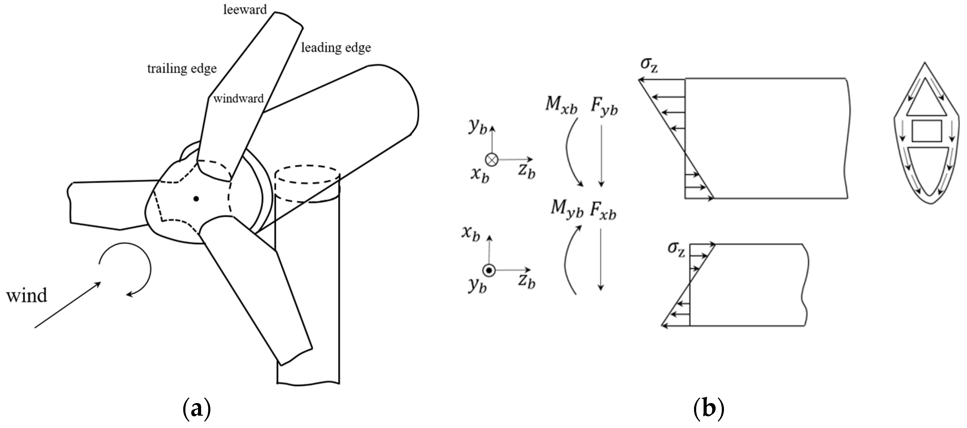
The wind turbine blade is shown in Figure 2a. Its cross section can be simplified as shown in Figure 2b, where the rectangle represents the main beam, and the semi-ellipse and triangle represent the leading and trailing edges, respectively. The section is symmetric to the y-axis. An equal-strength section design is used from the blade root to the tip.
According to the force characteristics [29], the blade is divided into two directions: waving and shimmy. In the waving direction, there are windward and leeward sides. In the shimmy direction, there are leading and trailing edges, as shown in Figure 3. In the waving direction, the strain formula is
ε w ( z ) = M w ( z ) E I x ( z ) x w ε l ( z ) = M l ( z ) E I x ( z ) x l
where ε w ( z ) and ε l ( z ) are the windward and leeward strains, respectively; M w ( z ) and M l ( z ) are the windward and leeward bending moments, respectively; and x w and x l are the distances from the windward and leeward outer surfaces to the neutral axis, respectively.
The formula for the strain ratio between the windward to the leeward is
ε w ( z ) ε l ( z ) = M w ( z ) M l ( z ) x w x l
The formula for the strain ratio between the leading edge to the trailing edge is
ε l e ( z ) ε t e ( z ) = M l e ( z ) M t e ( z ) y l e y t e
where ε l e ( z ) and ε t e ( z ) are the leading edge and trailing edge strains, respectively; M l e ( z ) and M t e ( z ) are the leading edge and trailing edge bending moments, respectively; and y l e and y t e are the distances from the leading edge and trailing edge outer surfaces to the neutral axis, respectively.
During the rotation of the blade, the leading edge is used to cut the wind. In this way, in a low-temperature and high-humidity environment, a large number of supercooled waters mainly accumulate at the leading edge, and eventually a thick ice layer is formed, as shown in Figure 3, which is the same as the phenomenon of icing on the blades in Figure 1. The icing of the leading edge causes the position of the center gravity of the blade to move toward the leading edge. Therefore, the strain ratio between the leading edge and the trailing edge is reduced, and the strain ratio at the windward side to the leeward side remains unchanged, so as to identify whether the blade is frozen according to this method. According to the strain ratio, the working state of the blade can be divided into three categories: the blade is in the normal condition, the leading edge of the blade is covered with ice, and damage occurs on the blade.

2.2. The Strain Ratio Index for Ice Detection

2.2.1. The Blade in the Normal Condition

For the convenience of calculation, it is assumed that the section is approximately symmetrical to the x-axis. When the blade is in the normal working condition, the waving direction is the same as the wind direction, and the shimmy direction is perpendicular to the wind direction. In this condition, M w ( z ) = M l ( z ) , M l e ( z ) = M t e ( z ) , and x w = x l , y l e y t e . Then, the strain ratio is
ε w ( z ) ε l ( z ) = x w x l = 1 ε l e ( z ) ε t e ( z ) = y l e y t e 1

2.2.2. The Leading Edge of the Blade Covered with Ice

During winter, the most common blade icing condition is that the largest amount of ice accumulates on the leading edge, while the other side has almost no ice. Due to surface freezing, the neutral axis moves to the leading edge. In this condition, M w ( z ) = M l ( z ) , M l e z = M t e z , and x w = x l , y le < y t e . Then, the strain ratio is
ε w ( z ) ε l ( z ) = x w x l = 1 ε l e ( z ) ε t e ( z ) = y l e y t e > 1

2.2.3. Damage Occurs on the Blade

When the wind turbine blade is damaged, x w x l , y l e y t e . Then, the strain ratio is
ε w ( z ) ε l ( z ) = x w x l 1 ε l e ( z ) ε t e ( z ) = y l e y t e 1

3. Blade Model Experiments

3.1. Experimental Blade Model

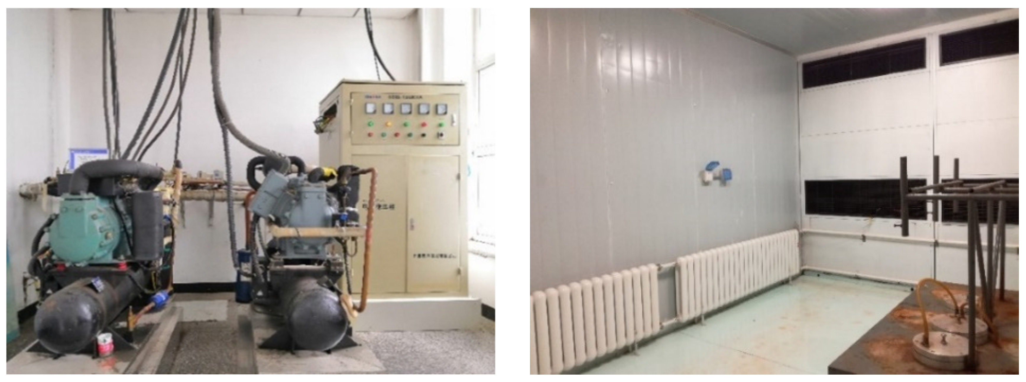
The experiment was performed in a low-temperature model laboratory with dimensions of 4.43 m (length) × 3.45 m (width) × 2.95 m (height), as shown in Figure 4. This laboratory allows for temperature adjustment within the range of −45 °C to 25 °C with a control accuracy of ±1 °C. For icing experiments, the temperature was stably set to −10 °C to simulate typical winter operating conditions. A 5 kW wind turbine blade model is used for the test, with its main components being vinyl epoxy resin and reinforced glass fiber reinforced plastic. Its key dimensions are as follows: the chord length of 2.65 m, maximum chord width of 0.3 m, tip width of 0.13 m, and blade root thickness of 0.05 m, as shown in Figure 5.
Ice was deposited on the blade’s upper surface via a controlled spray method, with 7 incremental icing cycles forming ice layers with thicknesses of 0.2 mm, 1.0 mm, 1.5 mm, 2.0 mm, 2.5 mm, 3.0 mm, and 3.5 mm, measured using a high-precision vernier caliper with an accuracy of ±0.01 mm. The ice morphology is shown in Figure 6.
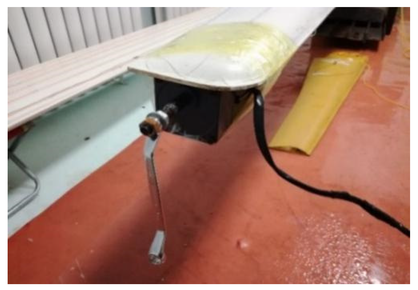
Owing to laboratory limitations, actual blade rotation under airflow was not simulated. Instead, to partially replicate the blade’s dynamic operating environment, the blade was fixed as a cantilever and tip-excited via a vibrator, as shown in Figure 7, with the vibration frequency set to 4 Hz. This setup focused on investigating the relationship between the icing of controlled thickness and the strain distribution under such dynamic conditions. In the experiment, FBG strain sensors were attached to symmetrical positions on the upper and lower surfaces of the blade, and data acquisition was performed using the SM130 FBG interrogator produced by Micron Optics (MOI) at a sampling frequency of 100 Hz, with each ice-covered state recorded for 100 s, and the strain ratio ε w ( z ) ε l ( z ) was computed for every 1 s. Raw data included wavelength shifts from FBG sensors, converted to strain values using pre-calibrated mechanical sensitivity coefficients. The test acquisition system is shown in Figure 8.

3.2. The Experimental Results

The vibration strain data are shown in Figure 9, which shows the values of the upper and lower surface strain data within 5 s. The upper surface strain value is opposite to the lower surface strain value. The strain value of the upper surface ranges from 53   μ ε to 53   μ ε , and the lower surface strain value ranges from 55   μ ε to 55   μ ε .
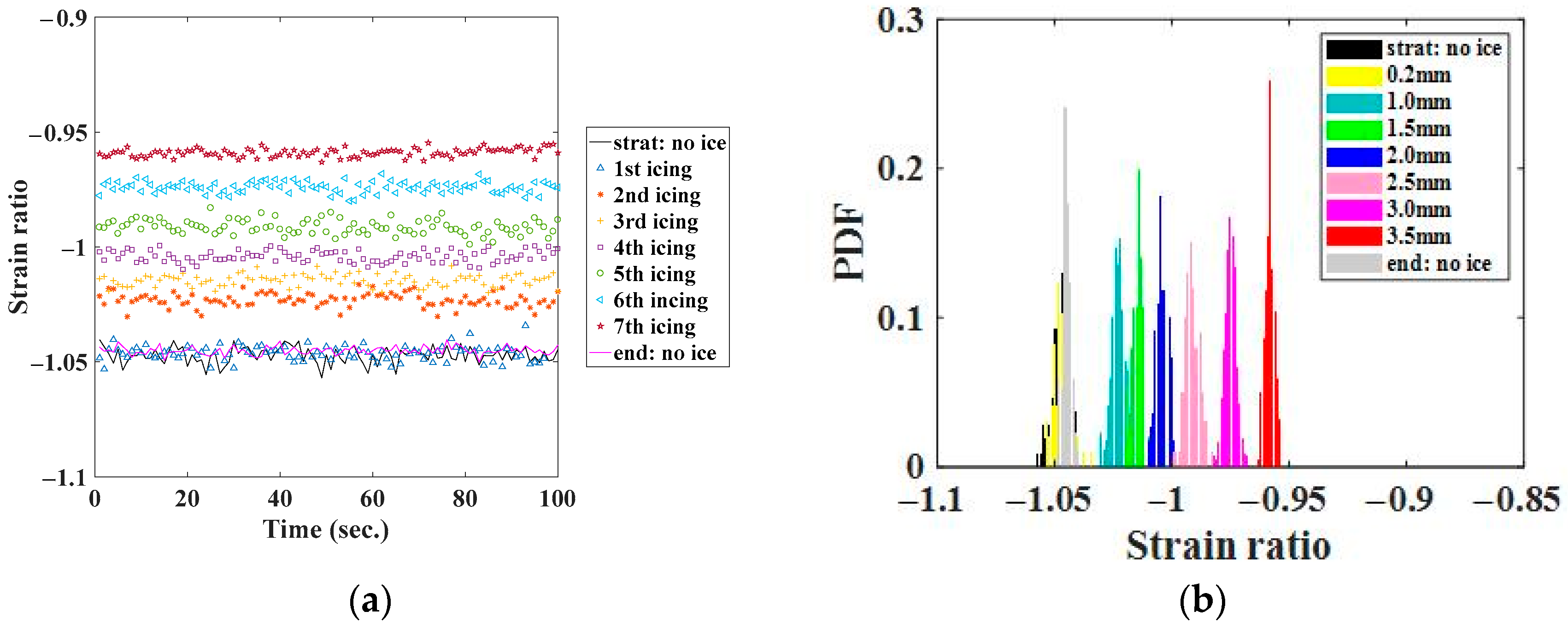
Figure 10a displays the strain ratios and Figure 10b shows the PDF of strain ratios under various ice-covered conditions. Without ice, the strain ratio is −1.05, which is defined as the initial value. Due to the asymmetry of the cross section and sensor installation position, the strain ratio is not equal to 1 in this experiment. At each icing thickness, the strain ratio has a relatively stable value.
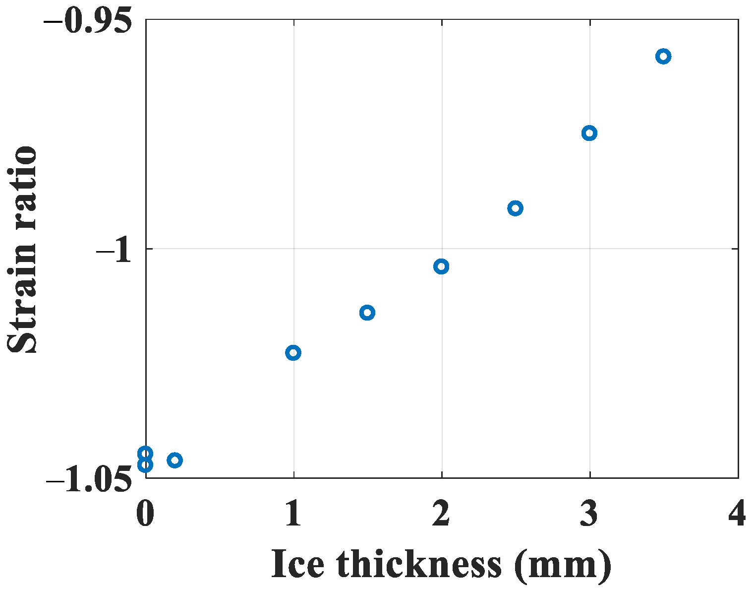
For ice thicknesses of 1.0 mm, 1.5 mm, 2.0 mm, 2.5 mm, 3.0 mm, and 3.5 mm, the corresponding strain ratios are −1.02, −1.01, −1.00, −0.99, −0.97, and −0.96, respectively. As depicted in Figure 11, the strain ratio presents a monotonic relationship with ice thickness, characterized by a gradual decrease in the absolute value of the strain ratio as the ice layer thickness increases. This observation confirms that the proposed strain ratio index maintains a strong correlation with ice coating thickness, thereby validating its potential as a reliable indicator for monitoring icing conditions on wind turbine blades.
The monotonic strain ratio changes with increasing ice thickness, aligning with the theoretical model proposed by Zhang et al. [21], which predicts a linear relationship between ice thickness and strain deviation. The mechanical analysis and actual experiments explicitly link neutral axis shifts to directional strain ratio changes, providing an interpretable explanation for Wang et al.’s observations that icing alters blade structural dynamics by changing mass distribution [16].
The 5 kW blade model experiment was conducted in a low-temperature laboratory with strictly controlled environmental parameters (e.g., temperature set to −10 °C, ice thickness precisely controlled from 0.2 mm to 3.5 mm, and vibration frequency of the vibrator fixed at 4 Hz). The laboratory experiment verified the fundamental mechanism of the strain ratio index and established a quantitative relationship between icing thickness and strain ratio changes, which was free from the complex interference of real-world conditions. The laboratory test on the 5 kW model established causality under controlled conditions by isolating icing as the sole variable, thereby verifying that strain ratio changes are directly induced by ice-driven neutral axis shifts. The physical mechanism underlying the method would remain unsubstantiated without this validation.

4. Field Test of Actual Wind Turbine for Ice Monitoring

4.1. The Monitoring System

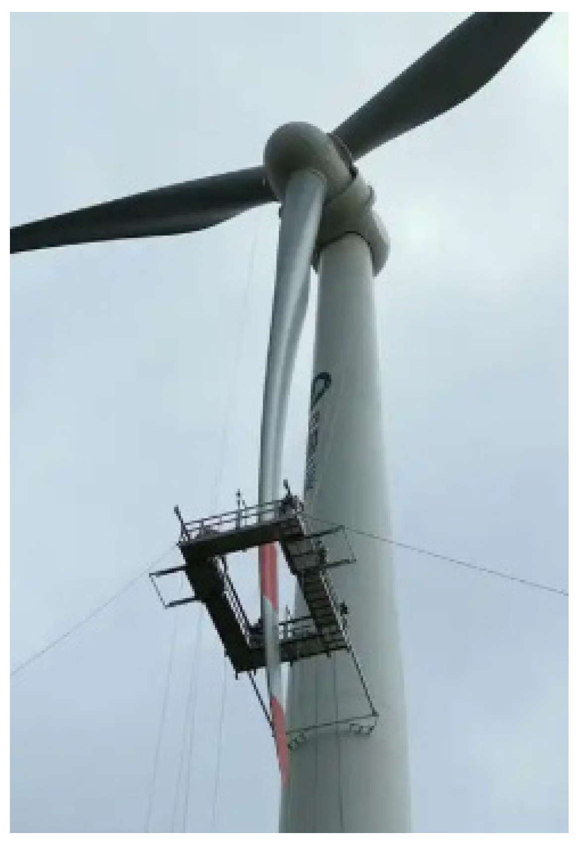
To further validate the icing monitoring ability of the proposed strain ratio index, a field test was conducted on an actual large-scale wind turbine. The test site was a wind farm in Shanxi Province of China, situated at an altitude ranging from 750 m to 1236 m. The tested wind turbine was the GW87/1500 direct-drive model manufactured by Goldwind Science & Technology Co., Ltd. (Beijing, China), featuring a rated power of 1.5 MW, an impeller diameter of 87 m, and a cut-in wind speed of 3 m/s, as shown in Figure 12.
When installing sensors at the root of the blades, the impeller was at the locked state, which refers to fixing it at a specific position through mechanical locking devices to ensure that the impeller could not rotate freely. One of the blades pointed to the ground and remained parallel to the tower, as shown in Figure 13, which was defined as the initial state of the blade. By adjusting the locking position of the impeller three times, the three blades were placed in the above-mentioned initial state in sequence to complete the calibration operation.
To eliminate the interference of temperature changes on the strain measurement, supplementary temperature sensors were introduced for compensation through a specific installation process. The temperature sensor was arranged perpendicular to the strain sensor, where the strain sensor is parallel to the blade axis; meanwhile, the temperature sensor was fixed at one end to ensure that it only responded to temperature changes without being affected by blade strain, thereby effectively achieving temperature compensation. The specific installation process of temperature sensors is shown in Figure 14a.
The sensor layout was designed to ensure data reliability as follows. On each blade, strain sensors were installed at the windward, leeward, leading edge, and trailing edge positions of the cross section, with a temperature compensation sensor adjacent to each strain sensor, as shown in Figure 14b. Longitudinally, all FBG sensors were located at 1.2 m from the blade root (Figure 14c). Each blade’s sensing array—comprising 4 strain sensors and 4 temperature sensors—was connected to an optical path, with the three blades’ optical paths linked to a grating modulator (Figure 14d), forming a quasi-distributed FBG sensing system for comprehensive blade monitoring.
To ensure data quality, MOI os3120 strain sensors, MOI os4100 temperature sensors, and an MOI sm130 demodulator, as shown in Figure 15, were selected after evaluating the anti-interference performance and long-term stability for harsh operating environments of wind turbines. After 1-year continuous monitoring, no clear signal drift and attenuation had been observed, which implies no significant impact on strain measurement accuracy. Additionally, four sensors per cross section were deployed to ensure the cross-validation stability and guarantee no individual sensor deviations.
For data quality control, multi-sensor deployment (e.g., 4 strain sensors per cross section) enabled cross-validation; individual sensor deviations were flagged and excluded. The MOI sm130 demodulator, fixed to the hub and rotating with the impeller, collected sensor data at a 100 Hz sampling frequency. The detailed configuration of the monitoring system is illustrated in Figure 16. It should be noted that partial loss of the wind turbine blade monitoring data occurred due to factors such as maintenance of the test wind turbine and large-scale power outages in the wind farm. The specific time periods of valid data retained were as follows: 2 September 2016–22 September 2016; 26 October 2016–20 February 2017; and 2 April 2017–6 July 2017.

4.2. Strain Value Characteristics of 1.5 MW Wind Turbine Blades

The state of the wind turbine can be divided into three states, which have different characteristics of strain data.
First, when the wind turbine is off and the blades are not rotating, the only load on the blades is gravity. The blade strain value is affected by the attitude when the blades stop rotating, as shown in Figure 17.
Second, when the blades are rotating, the loads on the blades are gravity and wind. In this state, the strain values are shown in Figure 18, which shows that the windward and leeward strain values range from −200 με to 200 με, and the leading edge and trailing edge strain values range from −150 με to 150 με. The periodicity is mainly caused by the rotation of the blade.
Third, when the wind turbine is powered on, the load on the blades are mainly wind and gravity. The wind load increases with the wind speed as shown in Figure 19a,b, which illustrates that the strain has different characteristics on each side. On the windward side, there is only a positive tensile strain, which is about 170 με, and on the opposite side, the negative pressure strain is about −150 με. In the direction of the shimmy, the leading-edge strain values range from −170 με to 170 με, and the trailing edge strain values range from −140 με to 230 με. The vibration in the waving direction is mainly affected by both wind force and impeller rotation. The shimmy direction is typically perpendicular to the wind, and its vibration is basically unaffected by wind speed and only affected by impeller rotation.
In addition to the above three states, the transitions between states in the long-term service of the wind turbine are worthy of attention and can be divided into three types.
First, as the wind speed gradually increases and exceeds 3 m/s, the wind turbine changes from shutdown to power-on state. The strain–time history curves in this process are shown in Figure 20, which shows that the strain values change from periodic to positive at the windward side, and the strain values change from periodic to negative at the leeward side in the waving direction; additionally, the amplitude and frequency increase significantly in the shimmy direction.
Second, when the wind speed gradually decreases to lower than 3 m/s, the wind turbine changes from the power generation state to the stop or stop rotation state. As shown in Figure 21, the windward strain value changes from 72 με to periodic with an amplitude of −215 με to 215 με. Eventually, it becomes a fixed value of −256 με. Similarly, the strain values change from periodic to a fixed value in the shimmy direction.
Third, when the wind speed is greater than 16 m/s, the wind turbine will protect itself from excessive aerodynamic loads by initializing downtime. In this case, the state of the wind turbine changes from normal power generation to powered off. The corresponding strain–time history curves for each side of the blade during this process are shown in Figure 22.

4.3. Ice Coating Detection of the Blade Based on the Measured Strain Values

The operation of blade is stable when the wind speed is greater than 8 m/s and the wind turbine is at full power. The corresponding strain values measured by FBG sensors are shown in Figure 23. The red line in the figure represents the result of linear fitting to the data, which shows that the strain values have an obvious linear relationship. The strain ratios in the waving direction and shimmy direction are the slopes of the fitted lines of strain data, which are −1.058 and −1.053, respectively.
The strain ratio data corresponding to the windspeed in different states are extracted, as shown in Figure 24. Figure 24a shows the state where the wind turbine is powered off and the blades are not rotating. At that time, the strain ratio is a fixed value relating to the attitude when the blades stop rotating. Figure 24b shows the state where the wind turbine is powered off and the blades are rotating. The waving direction strain ratio is close to −1, and the shimmy direction strain ratio is close to −0.85. As the wind speed increases, the range of the strain ratio gradually becomes smaller. As indicated in Figure 24c, when the wind turbine is powered on, the strain ratio in the shimmy direction remains stable at approximately −0.93 and in the waving direction is around −1.1. It can be observed that the amplitude in the shimmy direction is significantly smaller than the waving direction. The reason is that the blades need to adjust the sweeping area by changing their posture, and the wind turbine also needs yaw to align with the wind direction. These operations mainly affect the change of strain in the waving direction.
Based on the strain ratio, the long-term monitoring data of wind turbine blades are sorted by month, as shown in Figure 25, which shows the strain ratios in the waving and shimmy directions for September 2016, October 2016, November 2016, December 2016, January 2017, February 2017, April 2017, May 2017, and June 2017. The strain ratio in the waving direction is windward versus leeward, and the strain ratio in the shimmy direction is leading edge versus trailing edge. From Figure 25, the following information can be obtained:
(1)
When the wind speed is greater than 8 m/s, the change of strain ratio data in the waving direction is relatively stable, and the value trends to −1. When the wind speed is less than 8 m/s, the data vary widely. The reason is that when the wind speed is low, the wind turbine needs to adjust the blade angle to change the sweep area. Therefore, the strain in the waving direction changes frequently.
(2)
The strain ratio in the waving direction has basically no change with the month. Since the strain in the waving direction mainly reflects the change of the blade structure, it can be considered that the blades are not damaged in the testing period.
(3)
From September to October 2016, and June 2017, the strain ratio in the shimmy direction is basically maintained at a fixed value of −0.93 and does not vary with the wind speed because the shimmy direction is almost perpendicular to the leading and trailing edges, basically unaffected by wind speed and only affected by impeller rotation and icing.
(4)
The strain ratio changes greatly in the shimmy direction from November 2016 to May 2017. The strain ratio increases with time from November 2016 to February 2017. By February 2017, the strain ratio reaches a maximum of −0.34 and then gradually decreases. The strain ratio in June 2017 is basically the same as in September 2016.
The histogram of the probability distribution function (PDF) is obtained based on the calculation results of the wind turbine strain ratio data of September 2016, December 2016, February 2017, April 2017 and June 2017, as shown in Figure 26. It can be seen from Figure 26 that the maximum probability value of the strain ratio in the waving direction is −1, and there is no obvious change trend with time. In September 2016 and June 2017, the strain ratio in the shimmy direction is −0.93. The range of strain ratios in February 2017 is larger, with the main areas being [−0.8, −0.6], [−0.6, −0.4], and [−0.4, −0.33]. The strain ratio in April 2017 is mainly between −1 to −0.8. In the waving direction, the strain ratio is always −1 regardless of the month. In the shimmy direction, the absolute value of strain ratio decreases in the winter months, indicating that the neutral axis shifts toward the leading edge. Based on the above theoretical analysis, it can be predicted that icing occurs on the leading edge of the blade during November 2016 to May 2017. Moreover, the maximum amount of icing appears in February 2017.
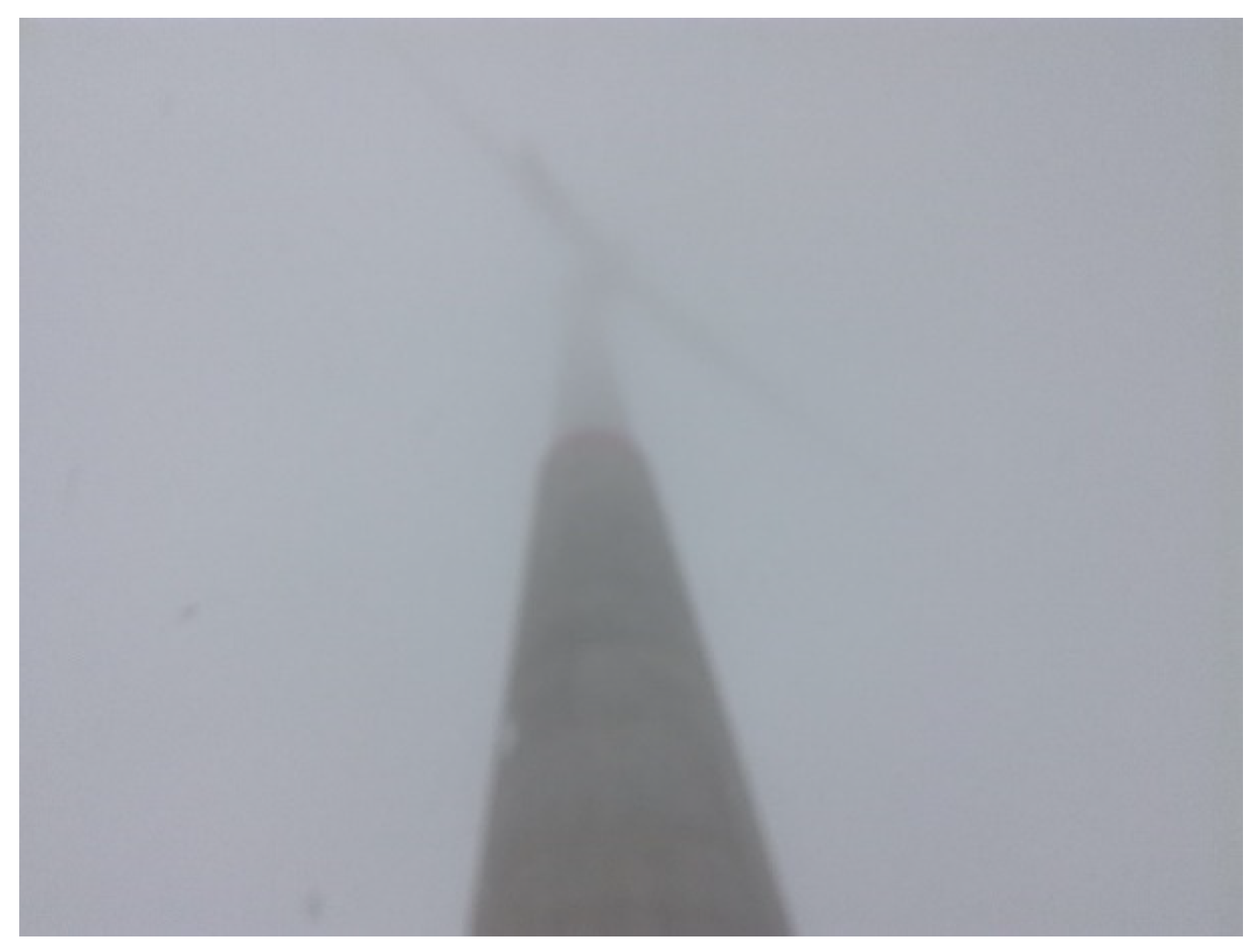
The test wind turbine is located in a mountainous area with a relatively high-altitude of 1100 m. It is cold in winter and prone to fog, snowfall, and other weather, as shown in Figure 27. In order to verify the icing prediction results of the above method, a photograph of the blade is taken on 8 January 2017, as shown in Figure 28, which shows that the leading edge of the blade is covered with ice. This illustrates that the proposed strain ratio index can effectively predict the icing of blades.
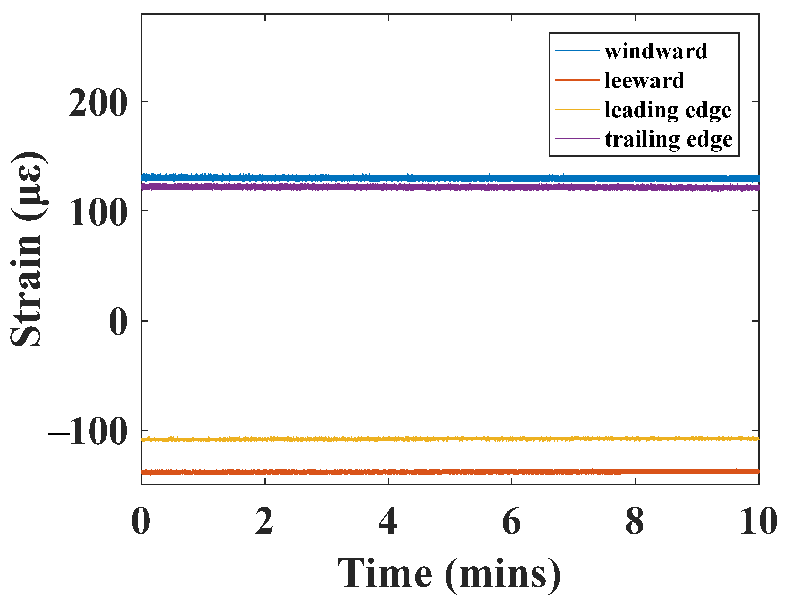
In order to better evaluate the ice coverage state of the blade, strain ratios on different dates with approximately the same wind speed are compared, as shown in Figure 29. The wind speed is about 8 m/s, and the strain ratio recording time is 10 min. In Figure 29a, the strain ratio in the waving direction changes little and is close to −1. However, the strain ratio in the shimmy direction varies greatly as shown in Figure 29b, which shows that the strain ratio gradually increases from −0.95, reaches a maximum of −0.36, then gradually decreases and finally returns to −0.95. This trend has good correlation with Figure 26b. Therefore, the change in the strain ratio is mainly due to the difference in ice thickness on the blade. The greater the thickness of the ice coating, the greater the change in the strain ratio.

4.4. Empirical Threshold for Icing Detection Criteria

As elaborated above, icing and damage will induce distinct strain ratio patterns due to different mechanical effects as follows:
(1)
Ice primarily accumulates at the leading edge, shifting the neutral axis toward the leading edge. This process selectively affects the shimmy direction strain ratio (i.e., leading edge strain/trailing edge strain) with the absolute value reducing from −1.05 to −0.34 (as shown in Figure 25 and Figure 26). In contrast, the waving direction strain ratio (i.e., windward strain/leeward strain) remains stable within [−1.2, −0.8] (as shown in Figure 25 and Figure 26), indicating that icing does not disrupt structural symmetry in the waving direction.
(2)
Blade damage (e.g., cracks) disrupts the overall structural integrity, affecting strain distributions in both directions. This process will cause the strain ratios in both waving and shimmy directions to deviate from the baseline ranges with irregular fluctuations, which is the typical difference from the icing induced strain ratio changes.
Based on the changes of the strain ratio in the waving and shimmy directions of the blades, the state of the blade ice coating can be evaluated. Empirical thresholds are established to classify states under stable 8 m/s wind conditions.
Table 1 shows the threshold-based differentiation criteria to classify icing and damage states. It should be noted that this study was conducted under the premise of a healthy blade without pre-existing damage, and using the proposed method could reliably identify icing states based on the strain ratio changes in both waving and shimmy directions. However, the abovementioned empirical criteria might not yet distinguish between “icing + damage” and “damage alone” due to their coupled effects. To address this issue, future work could include integrating frequency-domain analysis (e.g., vibration frequency shifts caused by damage or icing) to enhance the differentiation accuracy.
Gonzalez and Frövel demonstrated that FBG sensors can effectively detect icing via strain changes, and their work focused on static ice thickness measurements [30]. This study advances this by introducing a dynamic strain ratio index, enabling real-time monitoring of icing under operational vibrations. The 1.5 MW wind turbine field test was conducted in a wind farm over 1 year with harsh conditions (e.g., fog, snow, and temperature variations). The field test verified the applicability, robustness, and long-term reliability of the proposed method in actual operating scenarios, where multiple uncontrollable factors would interact. The field test on the 1.5 MW turbine confirmed the effectiveness in complex environments where icing coexists with other variables (e.g., wind, temperature, blade motion). The method’s real-world applicability would remain unproven without field tests.

5. Discussion

5.1. Validation of the Assumption: Ice Accretion-Induced Neutral Axis Shift

This study directly focuses on establishing the strain ratio index as a feasible monitoring indicator for icing detection, and it has been continuously supported by theoretical analysis, lab experiments, and field tests. Theoretical mechanical analysis in Section 2 has shown that ice accumulation on the leading edge altered the cross-sectional mass distribution, which inherently shifted the neutral axis. This was a principle consistent with the classical beam theory and further validated by laboratory experiments and field tests. Laboratory experiments in Section 3 indicated that the strain ratio index showed a clear monotonic relationship with ice thickness in Figure 10 and Figure 11, which aligned with the theoretical analysis of neutral axis shift. Field tests in Section 4 further validated that the absolute values of strain ratio reduced in the shimmy direction (Figure 25 and Figure 26), and the changes correlated with visual observations of leading-edge icing (Figure 28). In summary, all the above findings of theoretical analysis, lab experiments, and field tests contributed to confirming the assumption that ice accretion leads to a shift in the neutral axis.

5.2. Validation of the Categorization of Ice Thickness Based on Strain Ratio

For laboratory experiments in Section 3, ice thickness was precisely measured using a high-precision caliper (with a sensitivity of ±0.01 mm) during low-temperature model tests of the 5 kW blade. By correlating the measured ice thickness (0–3.5 mm) with the corresponding strain ratio values (−1.05 to −0.96) as shown in Figure 11, we established a series of strain ratio thresholds to classify different icing severities. Therefore, the accuracy and reliability of the proposed method have been validated by direct physical measurement of ice thickness in laboratory experiments.
For the classification of thin/intermediate/thick ice in the field tests of Section 4, it relies on the empirical judgment due to the challenges of real-time ice thickness measurement on operating 1.5 MW blades. This is achieved based on the observed trend of strain ratio changes in laboratory experiments, which has also been verified by qualitative visual inspections (e.g., drone inspection images of leading-edge icing in Figure 28).
It should be noted that further validations should be performed for (1) defining clear quantitative criteria for thin/intermediate/thick ice based on actual ice thickness measurements, (2) optimizing strain ratio thresholds by integrating both ice thickness according to different blade dimensions, and (3) evaluating the generality of ice severity classification criteria.

5.3. Future Research on Integrating the Kalman Filter and Strain Ratio for Reducing Noise Disturbance

While the proposed strain ratio index could effectively indicate the icing states, it still shows more apparent dispersion in field tests compared to laboratory experiments, which might be primarily caused by measurement noises and complex disturbances. Kalman Filter (KF)-based techniques [31,32] have exhibited significant advantages in handling measurement noise, system uncertainties, and temperature-induced strain changes, which inspired the robust tracking of strain changes caused by icing effects in this study. Future work includes exploring the integration of KF techniques to enhance the robustness of using the proposed strain ratio metric to indicate icing states, which might be investigated from the following aspects:
(1)
Given that icing-induced neutral axis shifts form the mechanical basis of the strain ratio index, KF could be employed to dynamically track the neutral axis. This will help suppress noise-induced fluctuations in field measurement data and reduce ambiguity from overlapping strain ratio points under different conditions.
(2)
Beyond the current static temperature compensation by dedicated sensors, KF will integrate temperature-related state variables into the parameter estimation framework. This will enable more precise correction of dynamic temperature-induced strain changes, improving the stability of utilizing the strain ratio index under varying thermal environments.
The advantages of the proposed strain ratio index and integrating KF-based techniques are summarized as follows, particularly in the context of practical wind turbine icing monitoring scenarios:
(1)
The strain ratio index is derived directly from the mechanical behavior of the blade (neutral axis shift due to icing), with clear physical meaning, simplicity, and interpretability. It avoids complex model assumptions of linear system dynamics, making it more reasonable to implement and interpret in complex engineering applications.
(2)
As validated in both laboratory experiments (Figure 10 and Figure 11) and field tests (Figure 25 and Figure 26), the strain ratio index consistently captures icing-induced changes (e.g., reducing absolute values in the shimmy direction) despite noise, enabling possible indications of thin/intermediate/thick ice with high efficiency.
Although the proposed strain ratio index could imply the icing state as a physics-driven detection method, the integration of KF would better address the limitations of noise-induced data dispersion, including applying KF to denoise strain measurements and refining neutral axis tracking, which would enhance the robustness under complex in-field environments. The hybrid approach of strain ratio and KF would both leverage the simplicity and interpretability of mechanical property and the noise-suppression ability for robust engineering applications.

5.4. Future Research on Industrial Implementation

Although this study presented a prototype verification focusing on the feasibility of using the strain ratio index for ice detecting by laboratory tests and real-world applications under complex operating conditions, further research would be conducted to promote the wide application of the proposed method for wind turbine icing monitoring in the following aspects:
(1)
For algorithm optimization, a more robust data processing framework should be developed, incorporating adaptive filtering and machine learning algorithms to suppress noise and eliminate interference from non-icing factors. This will improve the anti-disturbance capability of the strain ratio index and enhance the generalization ability under different application scenes.
(2)
For methodology validation, more field tests to more types of wind turbines (e.g., 6.7 MW, 16.2 MW models) and diverse cold-region environments (e.g., high-altitude areas, coastal cold zones) would be considered to verify the universality of the method.
(3)
For industrial application, a complete workflow including automated icing state classification (thin/intermediate/thick ice) and action linkage with deicing systems should be established to form an autonomous icing monitoring, early warning, and decision-making system.

6. Conclusions

In this study, a new method for icing detection of wind turbine blades based on the strain ratio is proposed. The effectiveness of the method is verified by an experimental model and a field test of an actual 1.5 MW wind turbine. For the actual wind turbine, a quasi-distributed FBG icing monitoring system is designed and installed. Long-term strain data are collected, and the characteristic information of the data is analyzed. Some conclusions are obtained as follows:
  • A quasi-distributed FBG monitoring technology can be used to realize real-time and dynamic monitoring for large wind turbines. The packaged FBG strain and temperature sensors are placed inside the blade, enabling in-line quasi-distributed measurements, and the FBG demodulator can be mounted on the blade and rotated simultaneously with the blade.
  • There are six different states of large-scale wind turbines during long-term operation: wind turbines are off and blades do not rotate, wind turbines are off but blades rotate, wind turbines generate electricity normally, wind turbines change from off to power-on state, wind turbines change from power-on to off state, and wind turbines shut down quickly due to excessive wind speed. Based on the characteristics of strain data, the above six wind turbine operating states can be effectively identified.
  • The mechanically derived strain ratio is interpretability and the change of strain ratios in different directions can be used for icing detection, since the absolute value of strain ratio in the shimmy direction will decrease with the increase in the ice thickness on the blade, while the strain ratio in the waving direction remains unchanged.
  • Laboratory experiment and in-field wind turbine test validate the effectiveness and robustness of the proposed method under complex operation scenarios.

Author Contributions

Conceptualization, Y.T. and Y.X.; methodology, Y.T., Z.Z. and Y.X.; software, Y.T.; validation, Y.T. and Z.Z.; formal analysis, Y.T. and Y.X.; investigation, all; resources, X.W., W.L. and Y.X.; data curation, Y.T. and Z.Z.; writing—original draft preparation, Y.T., Z.Z. and Y.X.; writing—review and editing, X.W., W.L. and Y.X.; visualization, Y.T. and Z.Z.; supervision, X.W., W.L. and Y.X.; project administration, X.W. and W.L.; funding acquisition, X.W. and W.L. All authors have read and agreed to the published version of the manuscript.

Funding

This research was funded by the National Key R&D Plan Program of the Ministry of Science and Technology of China (Grant Nos. 2021YFF0501003 and 2021YFB3202905), and the Guizhou Provincial Department of Transport Science and Technology Project (Grant No. 2023-122-001).

Data Availability Statement

The data presented in this study are available upon request from the first author.

Conflicts of Interest

Authors Yadi Tian and Xiaojing Wang were employed by the company China-Road Transportation Verification & Inspection Hi-Tech Co., Ltd. Author Zhaohui Zhang was employed by the company CCCC Highway Consultants Co., Ltd. The remaining authors declare that the research was conducted in the absence of any commercial or financial relationships that could be construed as a potential conflict of interest.

Abbreviations

The following abbreviations are used in this manuscript:
FBGFiber Bragg grating
PDFProbability distribution function

References

  1. Wei, K.; Yang, Y.; Zuo, H.; Zhong, D. A review on ice detection technology and ice elimination technology for wind turbine. Wind Energy 2020, 23, 433–457. [Google Scholar] [CrossRef]
  2. Lehtomäki, V. Wind Energy in Cold Climates Available Technologies-Report; Task 19, Technical Report; IEA: Paris, France, 2018; Available online: https://www.researchgate.net/publication/305881044_IEA_Wind_Task_19_-_Available_Technologies_report_of_Wind_Energy_in_Cold_Climates (accessed on 1 July 2016).
  3. Hämäläinen, K.; Niemelä, S. Production of a numerical icing atlas for Finland. Wind Energy 2017, 20, 171–189. [Google Scholar] [CrossRef]
  4. Fang, H.; Wang, L. Fast ice detection for wind turbine blades via the langevin equation. Proc. J. Phys. Conf. Ser. 2016, 753, 072016. [Google Scholar] [CrossRef]
  5. Muñoz, C.Q.G.; Márquez, F.P.G.; Tomás, J.M.S. Ice detection using thermal infrared radiometry on wind turbine blades. Measurement 2016, 93, 157–163. [Google Scholar] [CrossRef]
  6. Douvi, E.; Douvi, D. Aerodynamic Characteristics of Wind Turbines Operating under Hazard Environmental Conditions: A Review. Energies 2023, 16, 7681. [Google Scholar] [CrossRef]
  7. Dalili, N.; Edrisy, A.; Carriveau, R. A review of surface engineering issues critical to wind turbine performance. Renew. Sustain. Energy Rev. 2009, 13, 428–438. [Google Scholar] [CrossRef]
  8. Blasco, P.; Palacios, J.; Schmitz, S. Effect of icing roughness on wind turbine power production. Wind Energy 2017, 20, 601–617. [Google Scholar] [CrossRef]
  9. Gao, L.Y.; Tao, T.; Liu, Y.Q.; Hu, H. A field study of ice accretion and its effects on the power production of utility-scale wind turbines. Renew. Energy 2021, 167, 917–928. [Google Scholar] [CrossRef]
  10. Contreras Montoya, L.T.; Lain, S.; Ilinca, A. A review on the estimation of power loss due to icing in wind turbines. Energies 2022, 15, 1083. [Google Scholar] [CrossRef]
  11. Chuang, Z.J.; Yi, H.; Chang, X.; Liu, H.X.; Zhang, H.D.; Xia, L.L. Comprehensive Analysis of the Impact of the Icing of Wind Turbine Blades on Power Loss in Cold Regions. J. Mar. Sci. Eng. 2023, 11, 1125. [Google Scholar] [CrossRef]
  12. Høyland, K.V.; Nord, T.; Turner, J.; Hornnes, V.; Gedikli, E.D.; Bjerkås, M.; Hendrikse, H.; Hammer, T.; Ziemer, G.; Stange, T. Fatigue damage from dynamic ice action–The FATICE project. In Proceedings of the 26th International Conference on Port and Ocean Engineering Under Arctic Conditions, Moscow, Russia, 14–18 June 2021. [Google Scholar]
  13. Rocchi, E. Modeling of the Trajectory of Ice Thrown from a Wind Turbine. Master’s Thesis, Universitat Politècnica de Catalunya, Barcelona, Spain, 2023. [Google Scholar]
  14. Nodeland, A.M.; Bredesen, R.E.; Byrkjedal, Ø. Risk of ice throw from wind turbines validated with data from field measurements using drones. In Proceedings of the IWAIS 2022–19th International Workshop on Atmospheric Icing of Structures, Montréal, QC, Canada, 19–23 June 2022. [Google Scholar]
  15. Kabardin, I.; Dvoynishnikov, S.; Gordienko, M.; Kakaulin, S.; Ledovsky, V.; Gusev, G.; Zuev, V.; Okulov, V. Optical Methods for Measuring Icing of Wind Turbine Blades. Energies 2021, 14, 6485. [Google Scholar] [CrossRef]
  16. Wang, P.; Zhou, W.; Bao, Y.; Li, H. Ice monitoring of a full-scale wind turbine blade using ultrasonic guided waves under varying temperature conditions. Struct. Control Health Monit. 2018, 25, e2138. [Google Scholar] [CrossRef]
  17. Zheng, D.S.; Li, Z.Y.; Du, Z.Y.; Ma, Y.; Zhang, L.; Du, C.; Li, Z.J.; Cui, L.Q.; Zhang, L.; Xuan, X.G.; et al. Design of Capacitance and Impedance Dual-Parameters Planar Electrode Sensor for Thin Ice Detection of Aircraft Wings. IEEE Sens. J. 2022, 22, 11006–11015. [Google Scholar] [CrossRef]
  18. Zhang, C.; Xiao, C.H.; Li, S.R.; Guo, X.W.; Wang, Q.; He, Y.Z.; Lv, H.Y.; Yan, H.K.; Liu, D.G. A Novel Fiber-Optic Ice Sensor to Identify Ice Types Based on Total Reflection. Sensors 2023, 23, 3996. [Google Scholar] [CrossRef]
  19. Rizk, P.; Younes, R.; Ilinca, A.; Khoder, J. Wind turbine ice detection using hyperspectral imaging. Remote Sens. Appl. 2022, 26, 100711. [Google Scholar] [CrossRef]
  20. Yousuf, A.; Jin, J.Y.; Sokolov, P.; Virk, M.S. Study of ice accretion on wind turbine blade profiles using thermal infrared imaging. Wind Eng. 2021, 45, 872–883. [Google Scholar] [CrossRef]
  21. Zhang, Z.H.; Zhou, W.S.; Li, H. Icing estimation on wind turbine blade by the interface temperature using distributed fiber optic sensors. Struct. Control Health Monit. 2020, 27, e2534. [Google Scholar] [CrossRef]
  22. Davis, N.N.; Byrkjedal, O.; Hahmann, A.N.; Clausen, N.E.; Zagar, M. Ice detection on wind turbines using the observed power curve. Wind Energy 2016, 19, 999–1010. [Google Scholar] [CrossRef]
  23. Weijtjens, W.; de Oliveira Junior, A.F.; Cloet, B.; Yilmaz, Ö.C.; Devriendt, C. Large scale test of vibration based icing detection for wind turbines. Proc. J. Phys. Conf. Ser. 2024, 2647, 192008. [Google Scholar] [CrossRef]
  24. Szasz, R.Z.; Ronnfors, M.; Revstedt, J. Influence of ice accretion on the noise generated by an airfoil section. Int. J. Heat Fluid Flow 2016, 62, 83–92. [Google Scholar] [CrossRef]
  25. Ye, F.; Ezzat, A.A. Icing detection and prediction for wind turbines using multivariate sensor data and machine learning. Renew. Energy 2024, 231, 120879. [Google Scholar] [CrossRef]
  26. Jin, X.; Zhang, X.; Cheng, X.; Jiang, G.; Masisi, L.; Huang, W. A physics-based and data-driven feature extraction model for blades icing detection of wind turbines. IEEE Sens. J. 2023, 23, 3944–3954. [Google Scholar] [CrossRef]
  27. Cheng, X.; Shi, F.; Liu, Y.; Liu, X.; Huang, L. Wind turbine blade icing detection: A federated learning approach. Energy 2022, 254, 124441. [Google Scholar] [CrossRef]
  28. Tian, W.; Cheng, X.; Li, G.; Shi, F.; Chen, S.; Zhang, H. A multilevel convolutional recurrent neural network for blade icing detection of wind turbine. IEEE Sens. J. 2021, 21, 20311–20323. [Google Scholar] [CrossRef]
  29. Burton, T.; Jenkins, N.; Sharpe, D.; Bossanyi, E. Wind Energy Handbook; John Wiley & Sons: Hoboken, NJ, USA, 2011. [Google Scholar]
  30. Gonzalez, M.; Frövel, M. Fiber Bragg Grating Sensors ice detection: Methodologies and performance. Sens. Actuators A-Phys. 2022, 346, 113778. [Google Scholar] [CrossRef]
  31. Soman, R.; Majewska, K.; Mieloszyk, M.; Malinowski, P.; Ostachowicz, W. Application of Kalman Filter based Neutral Axis tracking for damage detection in composites structures. Compos. Struct. 2018, 184, 66–77. [Google Scholar] [CrossRef]
  32. Soman, R.; Malinowski, P.; Majewska, K.; Mieloszyk, M.; Ostachowicz, W. Kalman filter based neutral axis tracking in composites under varying temperature conditions. Mech. Syst. Signal Process. 2018, 110, 485–498. [Google Scholar] [CrossRef]
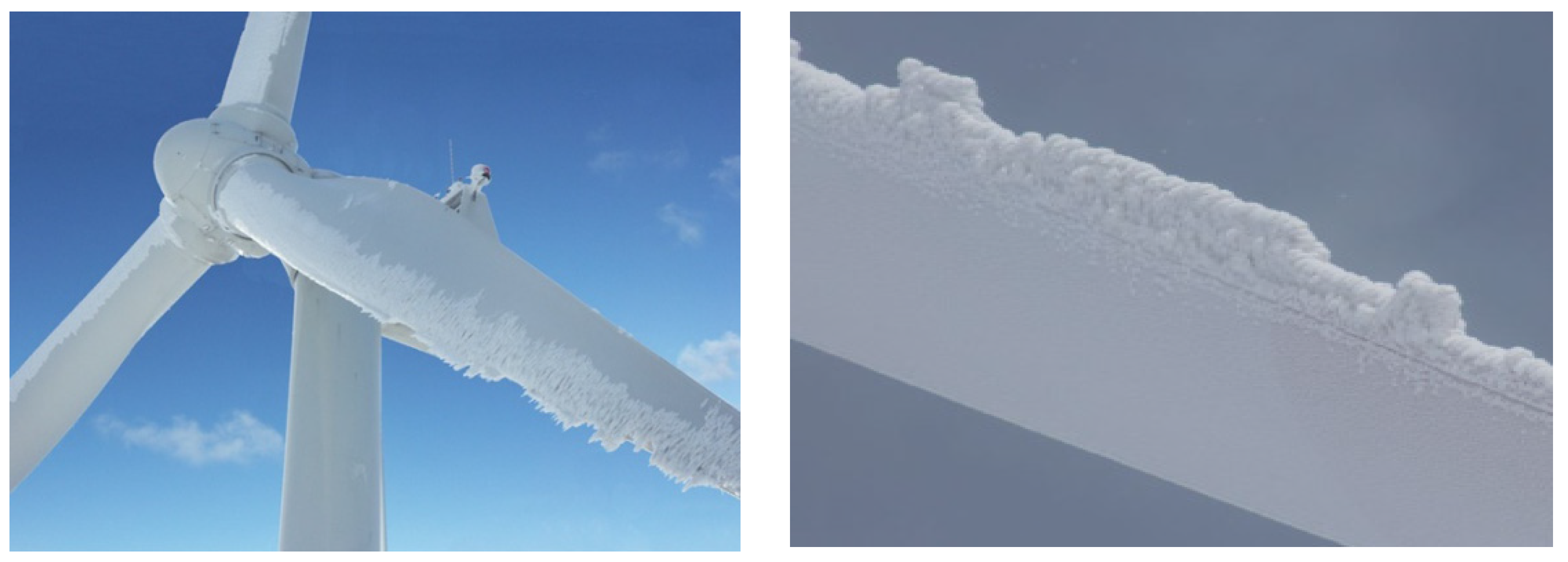
Figure 1. Icing on wind turbine blades.
Energies 18 04295 g001
Figure 2. Wind turbine blade: (a) simplified stereogram; (b) simplified analysis of the blade beam stress.
Energies 18 04295 g002
Figure 3. Simple analysis of icing on the leading edge of the blade.
Energies 18 04295 g003
Figure 4. The low-temperature model laboratory.
Energies 18 04295 g004
Figure 5. The experimental blade model: (a) the 5 kW wind turbine blade model; (b) the sensors are 1.5 m from the tip of the blade and are centered.
Energies 18 04295 g005
Figure 6. The icing layer on the upper surface of the blade during the test.
Energies 18 04295 g006
Figure 7. The test vibrator mounted at the tip of the blade.
Energies 18 04295 g007
Figure 8. Test data acquisition system.
Energies 18 04295 g008
Figure 9. Strain values within 5 s in the model test.
Energies 18 04295 g009
Figure 10. Strain ratios in the experiment: (a) strain ratios under different icing conditions (b) PDF of strain ratios at different ice thicknesses.
Energies 18 04295 g010
Figure 11. Relationship between the strain ratio and ice thickness.
Energies 18 04295 g011
Figure 12. The 1.5 MW test wind turbine.
Energies 18 04295 g012
Figure 13. Schematic diagram of the locked state of the wind turbine blade for calibration of the FBG sensors.
Energies 18 04295 g013
Figure 14. Arrangement of FBG sensors on the blade: (a) strain sensor and temperature sensor for compensation; (b) cross section installation position; (c) longitudinal installation position; (d) light path connection (The red positions denote strain sensors, and the green positions denote temperature sensors).
Energies 18 04295 g014
Figure 15. Data acquisition system: (a) MOI os3120 strain sensor; (b) MOI os4100 temperature sensor; (c) MOI sm130 fiber grating demodulator.
Energies 18 04295 g015
Figure 16. Construction of the quasi-distributed FBG icing monitoring system: (a) spring for protecting fiber from breaking by blade pitch; (b) ARK-1550 industrial computer; (c) power from the blade pitcher; (d) strain data acquisition and display.
Energies 18 04295 g016
Figure 17. Strain values when the wind turbine is powered off and the blades are not rotating.
Energies 18 04295 g017
Figure 18. Strain values when the wind turbine is powered off and the blades are rotating.
Energies 18 04295 g018
Figure 19. Strain and frequency when the wind turbine is powered on: (a) the strain values on the windward and leeward sides; (b) the strain values on the leading edge and trailing edge.
Energies 18 04295 g019
Figure 20. Strain values when the wind turbine changes from shutdown to power-on state: (a) the strain values on the windward and leeward side; (b) the strain values on the leading edge and trailing edge.
Energies 18 04295 g020
Figure 21. Strain values when the wind turbine changes from the power generation state to the stop or stop rotation state: (a) the strain values on the windward and leeward side; (b) the strain values on the leading edge and trailing edge.
Energies 18 04295 g021
Figure 22. Strain values when the wind turbine changes from the power generation state to powered off under high windspeed: (a) the strain values on the windward and leeward side; (b) the strain values on the leading edge and trailing edge.
Energies 18 04295 g022
Figure 23. Strain ratio in different directions of the blade: (a) the strain relationship between the windward and leeward; (b) the strain relationship between the leading edge and trailing edge.
Energies 18 04295 g023
Figure 24. Relationship between the strain ratio and the wind speed: (a) the strain ratio when the wind turbine is powered off and the blades are not rotating; (b) the strain ratio when the wind turbine is powered off and the blades are rotating; (c) the strain ratio when the wind turbine is powered on.
Energies 18 04295 g024
Figure 25. Strain ratio data of wind turbine blades in different months: (a) the strain ratio in September 2016; (b) the strain ratio in October 2016; (c) the strain ratio in November 2016; (d) the strain ratio in December 2016; (e) the strain ratio in January 2017; (f) the strain ratio in February 2017; (g) the strain ratio in April 2017; (h) the strain ratio in May 2017; (i) the strain ratio in June 2017.
Energies 18 04295 g025
Figure 26. PDF of strain ratios of wind turbine blades in different months: (a) the PDF of strain ratios in the waving direction; (b) the PDF of strain ratios in the shimmy direction.
Energies 18 04295 g026
Figure 27. The windy and snowy environment of the wind turbine on 6 January 2017.
Energies 18 04295 g027
Figure 28. Ice on the leading edge of the blade is observed on 8 January 2017.
Energies 18 04295 g028
Figure 29. Strain ratio of the blade on different days with wind speed 8 m/s: (a) the strain ratio in waving direction; (b) the strain ratio in shimmy direction.
Energies 18 04295 g029
Table 1. Threshold-based differentiation criterion to classify icing and damage states.
StateThreshold-Based Differentiation Criterion
(with a Fluctuation Range of ±20%)
Normal stateStrain ratio in both waving and shimmy directions stabilize within [−1.2, −0.8]
Icing state (No damage)
(1)
Waving direction: strain ratio remains within [−1.2, −0.8]
(2)
Shimmy direction: strain ratio deviates by >20% from −1.0, including:
  • Thin ice: [−1.0, −0.8]
  • Intermediate ice: [−0.8, −0.6]
  • Thick ice: [−0.6, 0]
DamageStrain ratio in both waving and shimmy directions exhibit either <−1.2 or >−0.8
Disclaimer/Publisher’s Note: The statements, opinions and data contained in all publications are solely those of the individual author(s) and contributor(s) and not of MDPI and/or the editor(s). MDPI and/or the editor(s) disclaim responsibility for any injury to people or property resulting from any ideas, methods, instructions or products referred to in the content.