Reverse-Demand-Response-Based Power Stabilization in Isolated Microgrid

Abstract

This paper introduces a reverse demand response scheme that uses electric vehicles in an isolated microgrid system, aiming to solve the renewable energy curtailment issue. We focus on an off-grid system where the system operator faces a stabilization problem due to surplus energy production, while electric vehicles seek to charge energy at a lower price. In our system model, the operator determines the incentive to encourage more charging facilities and electric vehicles to participate in the reverse demand response program. Charging facilities, acting as brokers, use a portion of these incentives to further encourage electric vehicle engagement. Electric vehicles follow the decisions made by the broker and system operator to determine their charging strategy within the system. Consequently, charging energy and incentives are allocated to the electric vehicles in proportion to their decisions. The paper investigates the economic benefits of individual participants and the contribution of power stabilization by implementing a hierarchical decision-making heterogeneous multi-leaders multi-followers Stackelberg game. By demonstrating the existence of a unique Nash Equilibrium, we show the effectiveness of the proposed model in an isolated microgrid environment.

1. Introduction

With the introduction of distributed power resources, various power management approaches have been developed to enhance system efficiency and profitability [1]. In particular, power systems on isolated microgrids (i.e., physically isolated from the main grid) require proper power management schemes and resources considering the given environment to stabilize the system [2]. Since most isolated microgrids do not have enough thermal power plants, they rely on renewable energy resources (e.g., solar PV systems, wind turbines, etc.) to supply enough power in the system [3]. However, renewable energy is sensitive to environmental changes and hard to control, leading to situations where power generation is less or greater than the expected value. In such cases, system operators should trade power with the main grid to stabilize the system [4,5].

The volatility of renewable energy can cause overproduction in isolated microgrids, resulting in issues like over-voltage, frequency instability, and network imbalances [6,7]. To address this problem, system operators propose several solutions: (i) renewable energy curtailment—temporarily turning off renewable generators [8], (ii) exporting excess power back to the main grid [9], and (iii) utilizing energy storage systems (ESSs) or converting it to hydrogen energy to manage the excess production efficiently.

First, renewable energy curtailment has the advantage that it can be immediately implemented. However, it results in financial loss and hinders carbon reduction efforts [6]. For the case of the HVDC approach, it is efficient in exchanging surplus power between the main grid and enhancing power reliability. However, the high installation cost of the required equipment makes it infeasible to preserve the profits of renewable energy. Lastly, another possible approach is to utilize storage to stabilize the power system. ESS and hydrogen storage devices have the advantage that they can easily control surplus renewable energy generation. However, constructing such equipment remains economically costly and entails safety risks such as explosion [10]. Additionally, water electrolysis technology is not yet commercialized.

Conventional demand response (DR) programs are primarily designed to reduce peak demand, but this approach is counterproductive in isolated microgrids experiencing surplus renewable energy. Reducing load during periods of overgeneration can exacerbate renewable curtailment and lower system efficiency. Several studies have highlighted the limitations of conventional DR under high renewable penetration [11], and proposed demand flexibility mechanisms that better align load with generation [12]. In contrast, reverse demand response (reverse DR, i.e., a variant of conventional demand response in which consumers are incentivized to increase rather than reduce their power consumption) programs incentivize increased consumption during such periods, offering a more suitable strategy for mitigating curtailment. Therefore, a reverse DR program has been proposed to address the issue of surplus renewable generation in isolated microgrids [13,14].

As a potential solution, we suggest a reverse DR scheme as a key strategy to solve the issue of excessive generation of renewable energy. As previously defined, a reverse DR program refers to a scheme in which consumers receive incentives to adjust their power consumption and contribute to stabilize the system [15,16]. An example of practical implementation can be seen in Arizona Public Service (APS), where such a program has been used to reduce solar energy curtailment when electricity prices are negative [17]. However, negative electricity prices are not frequent occurrences, and it remains challenging to determine the incentive price that effectively motivates power consumers to participate in the program. Additionally, most power consumers do not have controllable power resources during over-generation events. Furthermore, conventional programs do not consider the profit structure of users who participate in the program.

To overcome these challenges, we propose a reverse DR program specifically designed for isolated microgrids, utilizing electric vehicles (EVs) and their charging facilities. EVs are a type of vehicle powered by lithiumion batteries that can be autonomously charged and discharged. Due to their unique characteristics, such as easy charging and discharging capabilities, EVs can be utilized in various ancillary services, including vehicle-to-grid (V2G), grid-to-vehicle (G2V), and regulation up and down events [18,19,20,21]. For example, Ran et al. [18] proposed a DR policy using shared EV services and demonstrated that this scheme could reduce total costs by approximately 3%. Solanke et al. [19] also highlighted various ancillary services that could be managed with EVs, such as power backup, frequency regulation, and loss minimization. The paper demonstrated that incorporating EVs at different stages of the power system could increase system efficiency and reduce operation costs. As highlighted by Das and Kayal [21], the benefits to utilities significantly increase with greater participation of EV users in V2G services, especially when charging operations are coordinated rather than managed independently. Consequently, this underscores the importance of user cooperation and centralized scheduling in utilizing EVs as flexible demand-side resources. Considering EV’s characteristics, we can conclude that EVs are the most suitable power resource for operating a reverse DR program. However, unlike other power resources, it is essential to consider user behavior and preferences when implementing actual reverse DR programs.

Although several studies have investigated demand response mechanisms involving EVs [18,19,20,21] or applied game-theoretic approaches such as Stackelberg models to microgrid energy management [22,23,24], few conventional studies have specifically focused on reverse demand response tailored f or isolated microgrids with surplus renewable generation. Also, conventional models typically do not account for the hierarchical and strategic interplay among system operators (SOs), electric vehicle charging facilities (EVCFs), and EV owners.

In this paper, we conduct a comprehensive analysis of EVs to construct a reverse DR mechanism tailored for isolated microgrids. We develop a hierarchical game-theoretic model that captures the economic interests and strategic decisions of key participants—namely, the SO, EVCFs, and EV owners. The primary goal of this study is to address the challenge of surplus renewable energy generation by deriving optimal incentive strategies that balance power reliability with individual economic motivations. Furthermore, our model aims to validate the operational feasibility of reverse DR while ensuring incentive compatibility across all stakeholders.

The contributions of this paper are summarized as follows:

• By proposing a new energy management model, we show that it is possible to solve energy curtailment issues in an isolated microgrid.
• By analyzing the relationship between the leaders (i.e., the system operator and EVCFs) and the followers (i.e., EVCFs and EVs), we propose various analytical models suitable for adopting a reverse demand response mechanism in an actual power system.
• In the paper, we mathematically model a system with three types of players: the system operator, EVCFs, and electric vehicles with different interests. By showing the Nash Equilibrium of the model, we prove that it is possible to achieve the optimal strategy for each individual participant in the system.
• To analyze the effectiveness of the proposed operation scheme, we show an operating strategy of followers and power supplement in the system by varying the value of the system operator’s incentive. This approach allows us to determine the appropriate incentive price and demonstrate the feasibility of implementing the reverse DR scheme in an actual power system.

The rest of this paper is organized as follows: In Section 2, we introduce the proposed reverse DR scheme, providing details of the utility function of market participants in the system. Then, in Section 3, we explain the system operation using two-stage Stackelberg game theory. Following that, in Section 4, we show the performance of the proposed power operation scheme using an actual dataset. Finally, we summarize the main conclusions of the paper in Section 5.

2. System Model

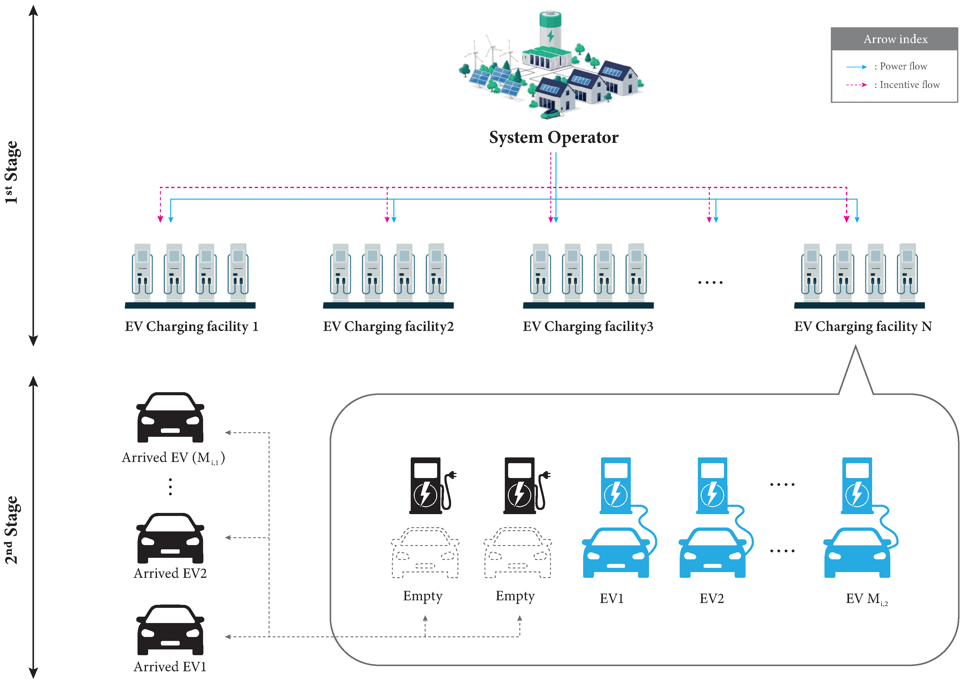
In our study, we focus on an isolated microgrid that is physically separated from the main grid and relies on renewable energy and distributed power resources to meet its power requirements. However, we encounter a situation where power generation from renewable energy exceeds the expected value. To address this issue, we propose controlling the power consumption of EVs as illustrated in Figure 1.

As shown in Figure 1, our proposed reverse DR scheme involves three participants: (i) EVs, (ii) EVCFs, and (iii) SO. Additionally, the reverse DR program is triggered when the renewable energy generation exceeds the expected demand within the isolated microgrid. In such surplus conditions, the SO detects the imbalance and initiates a reverse signal that activates the demand-side management mechanism. Specifically, the SO broadcasts incentive-based charging signals to EVCFs, encouraging increased electricity usage to absorb the excess generation. This initialization procedure ensures that the reverse DR mechanism is only deployed when system stability is threatened by overproduction.

In this system, EVs are categorized into two groups. The first group consists of EVs that have already received charging services before implementing the reverse DR program, and the second group consists of newly arrived EVs that decide to charge energy after the program is organized. EVCFs play the role of brokers, determining the charging price and incentives to be paid to EVs. They consider the profit per unit of EV and the inflow rate to maximize their own profits. The SO’s main objective is to stabilize the power supplement by increasing the overall power consumption of EVs.

In this paper, we focus on a scenario where the SO is the sole power supplement user, the only entity concerned about power reliability. Before renewable energy curtailment occurs due to increased power generation, the SO pays incentives $\widehat{p}$ to EVCFs to encourage more power consumption. For each $i\in {\mathcal{M}}_i$, we define $M_{i,1}$ as EVs that have previously received charging services at EVCF i, and $M_{i,2}$ is a set of newly arrived EVs at EVCF i. Although pricing policies of EVCF i can typically influence the inflow rate of other EVCFs in the market, we assume an environment where EVs are sufficiently supplied, and the pricing policy set by EVCF i does not affect the inflow rate of other EVCFs. As a result, EVCF i aims to determine the proper incentive $p_i$ solely considering its own profit factors.

However, we still consider the risk that charged EVs stop their charging services and move to other EVCFs if incentives for reverse DR are provided differently to EVs. To address this issue, we ensure that incentives should be paid equally to the EVs different groups. Furthermore, to prevent strategic manipulation, we assume that EV users cannot artificially interrupt and restart charging to increase their incentive-eligible volume. Instead, incentives are applied only to additional demand beyond the pre-committed or ongoing charging amount. It is also assumed that charging requests are either prepaid or logged upon initial connection and cannot be reset for the purpose of reclassification.

2.1. Utility Function of EVs

In this section, we analyze the utility function of EVs, which is influenced by the incentives provided by EVCFs.

2.1.1. Group 1: EVs Being Charged

From the viewpoint of EVs that are being charged, the occurrence of the reverse DR signal indicates a decrease in the expected cost for charging energy, which provide them additional profit through the charging service. From the SO’s perspective, conventionally charged EVs do not significantly impact the reliability of the power system. However, if incentives are not provided to these EVs, they will stop charging service and attempt to charge energy from other EVCFs. To avoid this scenario, we ensure that incentives are provided equally to EVs in both group 1 and group 2. In this environment, the strategies of EVs are primarily focused on determining the quantity of charging energy they consume rather than balking the facility.

For each $j\in M_{i,1}$, we define $E_j$ as the amount of energy that EV j initially planned to charge. Here, ${\alpha }_j$ represents the additional charging energy that EV j decides to charge. In the given environment, EVs aim to determine the optimal additional charging energy ${\alpha }_j$ that maximizes their own profit. The decision-making process for EV j is as follows:

$${\widehat{U}}_{1,j}\left({\alpha }_j\right)=p_i{\alpha }_j+(1-\beta )c_i(E_j+{\alpha }_j)-c_{dis}{\left({\displaystyle \frac{E_j+{\alpha }_j}{e}}\right)}^2.$$

(1)

In Equation (1), $p_i$ represents the incentive provided by EVCF i when EVs participate in the reverse DR event. Thus, $p_i{\alpha }_j$ signifies the monetary profit directly received by EVCF i for each unit of additional charging energy ${\alpha }_j$ contributed by EV j. In our system, we assume that both EVs and EVCFs share the cost of charging power. Here, we set the environment that both EVs and EVCFs share the cost of charging power. Therefore, the term $(1-\beta )c_i(E_j+{\alpha }_j)$ denotes the portion of the cost that an EV j pays for charging energy. Here, $c_i$ represents the energy selling price of EVCF i, and $E_j$ is the conventionally planned charging energy of EV j. Additionally, we introduce the auxiliary variable $c_{dis}$ to convert EVs’ dissatisfaction factor regarding the delay in charging time into monetary cost [25]. Here, the inconvenience of EVs that occurs due to the delay in charging time is modeled using a quadratic function as referred to in [22]. The charging time is calculated by dividing the charging amount per unit time e from the total charging energy $E_j+{\alpha }_j$. By adding the auxiliary variable $c_{dis}$, we could express the user’s discomfort in the monetary aspect as depicted in the equation.

2.1.2. Group 2: Newly Arrived EVs

After the reverse DR program is implemented, some EVs decide to receive charging services, which are regarded as group 2 in this paper. The main object of EVs in group 2 is to maximize their own profit by taking advantage of the incentives and charging energy at a lower price. The difference between EVs in group 1 and 2 is that group 2 does not have a predetermined amount of charging energy. Therefore, for each $j\in M_{2,j}$, the utility function of EV j is defined as follows:

$${\widehat{U}}_{2,j}\left({\alpha }_j\right)=p_i{\alpha }_j+(1-\beta )c_i{\alpha }_j-c_{dis}{\left({\displaystyle \frac{{\alpha }_j}{e}}\right)}^2.$$

(2)

In Equation (2), the utility function of EVs in group 2 is similar to EVs in group 1. However, $E_j$ is equal to 0 in the formula because EVs in group 2 are not being charged before. Therefore, EVs determine whether to charge energy by comparing the profit between the receiving charging service and leaving without the charging service. EVs make the decision based on the incentives and charging energy prices achieved by the reverse DR program.

2.2. Utility Function of EVCFs

In the system, the primary goal of EVCFs is to maximize their own profit as brokers. However, when a significant portion of incentives received from SO is provided to EVs, the per unit revenue of the EVCF will decrease. As a result, the revenue of the EVCF is determined by the portion of incentive and the overall inflow rate of EVs. Thus, for each $i\in N$, the utility function of EVCF i could be expressed mathematically as follows:

$$U_i\left(p_i\right)=\widehat{p}\sum _{j\in M_i}{\alpha }_j-p_i\sum _{j\in M_i}{\alpha }_j-\beta c_i(\sum _{j\in M_{i,1}}(E_j+{\alpha }_j)+\sum _{j\in M_{i,2}}{\alpha }_j)$$

(3)

In Equation (3), EVCF i determines the incentive $p_i$ to induce EVs participating in the reverse DR program. Here, $\widehat{p}$ refers to the incentive that EVCFs receive from the SO for organizing the reverse DR program. Therefore, $\widehat{p}{\sum }_{j\in M}{\alpha }_j$ represents the revenue that EVCF i earns by introducing the reverse DR program, and $p_i{\sum }_{j\in M}{\alpha }_j$ represents the incentive cost provided to EVs. Since $\beta$ refers to the portion that EVCF i pays for charging cost, the remaining part of the formula represents the charging fee borne partially by the EVCF. Through this equation, EVCF i determines a reasonable incentive $p_i$ by analyzing its own profit and monetary expenditure.

2.3. Utility Function of SO

As discussed in the previous section, the SO bears the responsibility of maintaining the reliability of the power system through the various management schemes (i.e., reverse DR program, ancillary services, optimal power flow, etc). From the SO’s perspective, the occurrence of renewable energy curtailment implies system instability and monetary loss. In this paper, we define the utility function of the SO by converting these loss factors into a monetary aspect as

$$U_{SO}\left(\widehat{p}\right)=(p_{carbon}-\widehat{p})\sum _{i\in N}\sum _{j\in M_i}{\alpha }_j.$$

(4)

Equation (4) represents the net profit that the SO obtains through the operation of the reverse DR program. In the equation, $p_{carbon}$ represents the profit per unit of power that the SO gains when preventing the occurrence of renewable energy curtailment. Additionally, $\widehat{p}$ denotes the incentive provided to EVCFs to organize the reverse DR program. In this environment, the SO determines the value of $\widehat{p}$ to maximize its own profit. By optimizing the incentive amount, the SO can effectively balance the reduction in energy curtailment and monetary losses with the cost of providing incentives to EVCFs.

3. Game-Theoretic Analysis

To effectively coordinate the strategic decisions of participants in the reverse DR program, we model the interaction as a two-stage Stackelberg game. This allows us to capture market participant’s objectives and find equilibrium-based operational strategies.

3.1. Preliminaries

Generally, Stackelberg game is one of the representative non-cooperative game models where participants have different utilities and are divided into leader and follower positions [26]. In the conventional scheme, the most important key point of the model is that followers are influenced by the leader’s decision and optimize their own strategy within it. Since the characteristics of this model are suitable for the power system environment, it could be widely used to derive optimal decision-making in various problems [22,23,24]. Here, the scheme is used to solve decision-making problems that could occur among participants. As the power system and market become more complicated, the application of this method also increases and is used in various fields.

In our problem, we consider the SO as the leader, and EVCFs assume the role of middle managers acting as both leaders and followers, while EVs in the system take on the role of followers. In the system, EVs submit their decision ${\alpha }_j$ to the EVCF, which aims to maximize their own profit. In the middle manager’s game, they determine a strategy $\mathbf{p}$ depending on the decisions of the EVs in the facility. Lastly, the SO determines the incentive $\widehat{p}$ that should be provided to EVCFs. In this situation, to avoid economically infeasible outcomes such as zero or negative effective electricity prices for EV users, we assume that the per-unit incentive is constrained by an upper bound. This ensures that the final charging price remains strictly non-negative, maintaining the economic feasibility and integrity of the reverse DR mechanism.

To achieve Nash equilibrium in the proposed Stackelberg game model, we use a backward induction approach. We first find the optimal strategy of the EVs from the follower-level game and apply this value to the utility function of the middle manager, optimizing it accordingly. Finally, the optimal values of followers and middle managers are applied to the leader’s utility function to calculate the optimal strategy of the leader.

3.2. Non-Cooperative Game of Follower—Case of EVs

Definition 1.

The best response function $B_{EV,j}\left({\alpha }_{1,j}\right)$ of EV j as a follower is the best strategy for buyer j achieved by the EVCF’s strategy $\mathbf{p}$. By definition, we have

$$\begin{array}{c}\hfill B_{EV,j}\left({\alpha }_{1,j}\right)=\underset{{\alpha }_{1,j}}{arg\; max}{\widehat{U}}_j({\alpha }_{1,j},\mathbf{p})\end{array}$$

(5)

Definition 2.

The optimal best response of the EV is determined as the optimal strategy ${\alpha }^{*}$ with the property given by the leader’s strategy $\mathbf{p}$. Therefore, we have

$${\alpha }_{1,j}^{*}=B_{EV,j}\left({\mathbf{p}}^{*}\right)\forall j\in M$$

(6)

Lemma 1.

The utility function of EV j is strictly concave and can derive a global optimal solution.

Proof. 

Given Equation (1), we have

$$\begin{array}{c}\hfill {\widehat{U}}_{1,j}\left({\alpha }_{1,j}\right)={\alpha }_{1,j}{p}_i+(1-\beta )c_i(E_j+{\alpha }_{1,j})-c_{dis}{\displaystyle \frac{{(E_j+{\alpha }_{1,j})}^2}{e^2}}.\end{array}$$

(7)

Taking the first and second derivatives of ${\widehat{U}}_{1,j}\left({\alpha }_{1,j}\right)$ with respect to ${\alpha }_{1,j}$, we have

$$\begin{array}{cc}\hfill {\displaystyle \frac{\partial {\widehat{U}}_{1,j}\left({\alpha }_{1,j}\right)}{\partial {\alpha }_{1,j}}}& =p_i+(1-\beta )c_i-2C_{dis}{\displaystyle \frac{(E_j+{\alpha }_j)}{e^2}}\hfill \end{array}$$

(8)

$$\begin{array}{cc}\hfill {\displaystyle \frac{{\partial }^2{\widehat{U}}_{1,j}\left({\alpha }_{1,j}\right)}{\partial {\alpha }_{1,j}^2}}& =-2C_{dis}{\displaystyle \frac{1}{e^2}}\hfill \end{array}$$

(9)

Given that the right side of Equation (9) always has a value less than 0, the utility function of EV j is strictly concave on ${\alpha }_j$ [27]. After proving that ${\widehat{U}}_{1,j}$ is concave, we could achieve the best response function of EV j by setting the right hand side of the Equation (8) as equal to zero.

$$\begin{array}{cc}\hfill & {\displaystyle \frac{\partial {\widehat{U}}_{1,j}\left({\alpha }_{1,j}\right)}{\partial {\alpha }_j}}=p_i+(1-\beta )c_i-2C_{dis}{\displaystyle \frac{(E_j+{\alpha }_{1,j})}{e^2}}=0\hfill \\ \hfill & \therefore {\alpha }_{1,j}^{*}={\displaystyle \frac{1}{2C_{dis}}}(p_i+(1-\beta )c_i)e^2-E_j\forall j\in M_{i,1}.\hfill \end{array}$$

(10)

In Equation (10), we could derive the optimal value of ${\alpha }_j^{*}$. As referred in Equations (1) and (2), the difference between the groups are receiving charging services conventionally. Therefore, it is possible to calculate the optimal value of newly arrived EVs using the same approaches as follows:

$$\begin{array}{cc}\hfill & {\displaystyle \frac{\partial {\widehat{U}}_{2,j}\left({\alpha }_{2,j}\right)}{\partial {\alpha }_{2,j}}}=p_i+(1-\beta )c_i-2C_{dis}{\displaystyle \frac{{\alpha }_{2,j}}{e^2}}=0\hfill \\ \hfill & \therefore {\alpha }_{2,j}^{*}={\displaystyle \frac{1}{2C_{dis}}}(p_i+(1-\beta )c_i)e^2\forall j\in M_{i,2}.\hfill \end{array}$$

(11)

In Equation (11), we could check utility function of EVs are concave function. Therefore, we could represent that ${\alpha }_{2,j}^{*}$ is the optimal solution of newly arrived EVs. □

Generally, the net profit that EVs obtain by participating in the reverse DR program should be greater than 0. In other words, EVs will not participate in the reverse DR program if the losses are greater than the profit. Therefore, after obtaining the optimal solution from each participant and evaluating their utility functions, we can determine EVs’ decisions based on their net profit.

3.3. Non-Cooperative Game of Leader—Case of EVCFs

Definition 3.

Depending on the best response function $B_{EV,j}\left(\mathbf{p}\right)$, it is possible to achieve an optimal strategy $p_i$ which is affected by the leader’s strategy $\widehat{\mathbf{p}}$. Under this condition, we have

$$\begin{array}{c}\hfill B_{EVCF,i}\left(\mathbf{p}\right)=\underset{p_i}{arg\; max}{U}_i(p_i,\widehat{\mathbf{p}}).\end{array}$$

(12)

Definition 4.

As discussed in the above section, the best responses of EVCF i is related to the leader’s strategy $\widehat{\mathbf{p}}$. In this case, we could depict EVCF i’s optimal value as follows:

$$\begin{array}{c}\hfill p_i^{*}=B_{EVCF,i}\left(\widehat{{\mathbf{p}}^{*}}\right)\forall i\in N\end{array}$$

(13)

Lemma 2.

We have to prove that the utility function of $U_i(p_i,\widehat{\mathbf{p}})$ is strictly concave on $p_i$. Here, we could show the concavity of the function and determine the optimal value using the same scheme depicted in Section 3.2.

Proof. 

In Equation (3), we could take the first and second derivatives of $U_i(p_i,\widehat{\mathbf{p}})$.

$$\begin{array}{cc}\hfill {\displaystyle \frac{\partial U_i(p_i,\widehat{\mathbf{p}})}{\partial p_i}}& ={\displaystyle \frac{M_i{e}^2}{2C_{dis}}}(\widehat{p}-p_i)-\beta c_i{\displaystyle \frac{M_i{e}^2}{2C_{dis}}}\hfill \\ \hfill & -\left[{\displaystyle \frac{M_i{e}^2}{2C_{dis}}}(p_i+\beta c_i)-\sum _{j\in M_{i,1}}{E}_j\right]\hfill \\ \hfill {\displaystyle \frac{{\partial }^2{U}_i(p_i,\widehat{\mathbf{p}})}{\partial p_i^2}}& =-{\displaystyle \frac{M_i{e}^2}{C_{dis}}}\hfill \end{array}$$

(14)

Here, EVCF i can propose optimal value of $p_i$ that maximizes its own profit by setting the right side of Equation (14) as 0.

$$\begin{array}{c}\hfill p_i^{*}={\displaystyle \frac{1}{2}}\widehat{p}+{\displaystyle \frac{C_{dis}}{M_i{e}^2}}\sum _{j\in M_{i,1}}{E}_j-\beta c_i\end{array}$$

(15)

□

3.4. Non-Cooperative Game of Leader—Case of SO

Definition 5.

Based on the optimal strategy of EV and EVCF, it is possible to calculate the optimal value that SO should present. At this time, the utility function of SO can be represented as follows:

$$\begin{array}{cc}\hfill U_{SO}\left(\widehat{p}\right)& =(p_{carbon}-\widehat{p})\sum _{i\in N}\sum _{j\in M_i}{\alpha }_j\hfill \\ \hfill & =(p_{carbon}-\widehat{p})\sum _{i\in N}[\sum _{j\in M_{i,1}}{\alpha }_j+\sum _{j\in M_{i,2}}{\alpha }_j]\hfill \\ \hfill & =(p_{carbon}-\widehat{p})\sum _{i\in N}[{\displaystyle \frac{M_i{e}^2}{2C_{dis}}}(p_i+\beta c_i)-\sum _{j\in M_{i,1}}{E}_j]\hfill \\ \hfill & =(p_{carbon}-\widehat{p})\sum _{i\in N}[{\displaystyle \frac{M_i{e}^2}{4C_{dis}}}\widehat{p}-{\displaystyle \frac{1}{2}}\sum _{j\in M_{i,1}}{E}_j].\hfill \end{array}$$

(16)

As depicted in Equation (16), it is possible to transform utility function according to the value of $\widehat{p}$. Here, it is possible to achieve an optimal strategy of SO using the same scheme as shown in the previous section.

$$\begin{array}{cc}\hfill {\displaystyle \frac{\partial U_{SO}\left(\widehat{p}\right)}{\partial \widehat{p}}}& =\sum _{i\in N}[{\displaystyle \frac{M_i{e}^2}{4C_{dis}}}(p_{carbon}-\widehat{p})\hfill \\ \hfill & -[{\displaystyle \frac{M_i{e}^2}{4C_{dis}}}\left(\widehat{p}\right)-{\displaystyle \frac{1}{2}}\sum _{j\in M_{i,1}}{E}_j]]\hfill \end{array}$$

(17)

$$\begin{array}{cc}\hfill {\displaystyle \frac{{\partial }^2{U}_{SO}\left(\widehat{p}\right)}{\partial {\widehat{p}}^2}}& =-\sum _{i\in N}{\displaystyle \frac{M_i{e}^2}{2C_{dis}}}\hfill \end{array}$$

(18)

In Equation (18), regardless of the value of $\widehat{p}$, we ensure that the second-derivative term is less than zero, which ensures that the utility of SO is strictly concave for $\widehat{p}$. Therefore, we could achieve the optimal value of $\widehat{p}$ by setting the first-derivative equation equal to zero.

$$\begin{array}{cc}\hfill & {\displaystyle \frac{M_i{e}^2}{4C_{dis}}}(p_{carbon}-\widehat{p})\hfill \\ \hfill & -[{\displaystyle \frac{M_i{e}^2}{4C_{dis}}}(\widehat{p}+(1-2\beta )c_i)-{\displaystyle \frac{1}{2}}\sum _{j\in M_{i,1}}{E}_j]=0\hfill \\ \hfill & \therefore {\widehat{p}}^{*}={\displaystyle \frac{1}{2}}{p}_{carbon}+C_{dis}{\displaystyle \frac{{\sum }_{i\in N}{\sum }_{j\in M_{i,1}}{E}_j}{{\sum }_{i\in N}{M}_i{e}^2}}\hfill \end{array}$$

(19)

Based on Equation (19), we could calculate the optimal value that could maximize SO’s profit.

4. Numerical Results

To validate the proposed model, we establish a simulation environment using the pricing data used in the actual system (i.e., carbon reduction incentive and EV charging price). To determine the carbon reduction incentive ($p_{carbon}$), we gathered two types of datasets: (i) carbon generation using the fossil fuel and renewable energy ($\Delta E_{{\mathrm{CO}}_2}$), (ii) carbon reduction incentive per CO₂/kWh ($I_{{\mathrm{CO}}_2}$). Generally, carbon emissions occur by the use of different fossil fuels. In [28], Spath et al. argued that coal combustion results in the production of CO₂ are 1022 g/kWh, 941 g/kWh, and 741g/kWh from the Average, NSPS, and LEBS systems, respectively. Furthermore, Mittal et al. showed that CO₂ emissions per unit of electricity are located between $0.82$ and $1.0$ kg/kWh in [29]. Currently, the trading price of carbon credits is more than USD 8–USD 88 per ton. Using the carbon emission and pricing data argued in [30,31,32], carbon incentive could be calculated using $\Delta E_{{\mathrm{CO}}_2}\times I_{{\mathrm{CO}}_2}$ and a set boundary between USD $0.00656$ and USD $0.080$ per kWh. The detail value of parameters are described in

Table 1. Simulation parameters to operate power in charging facility.

Simulation Parameters	Value
Incentive provided by EVCF i ($p_i$)	-
Additional charging energy of EV j (${\alpha }_j$)	-
Incentive provided by SO ($\widehat{p}$)	-
Weight factor of burden charging energy price ($\beta$)	0–1
Conventionally stored energy in EV j ($E_j$)	0 kWh–35 kWh
Auxiliary variable to transform user discomfort into monetary cost	0–0.5
Unit charging energy (e)	5 kWh–7 kWh
Carbon reduction incentive ($p_{carbon}$)	USD $0.00656$–USD $0.080$

.

4.1. Correlation Between Variables

As referred in Section 2, the decisions of market participants’ strategies are closely related to the amount of energy promised to be charged and the discomfort factor that occurs according to the charging delay of EVs.

In Figure 2, we illustrate the relationship between the SO’s incentive price and two auxiliary variables $C_{dis}$ and $E_j$. Equation (19) shows that $\widehat{p}$ is directly proportional to $C_{dis}$ and $E_j$. From the figure, we observe that $\widehat{p}$ tends to increase proportionally with the increment of $C_{dis}$. It is intuitively evident that the influence of $C_{dis}$ is greater than that of $E_j$. Therefore, we could assume that $C_{dis}$ has a greater impact on the SO’s decision-making than $E_j$. This hypothesis can be confirmed through the analysis of Equation (19) and the simulation results.

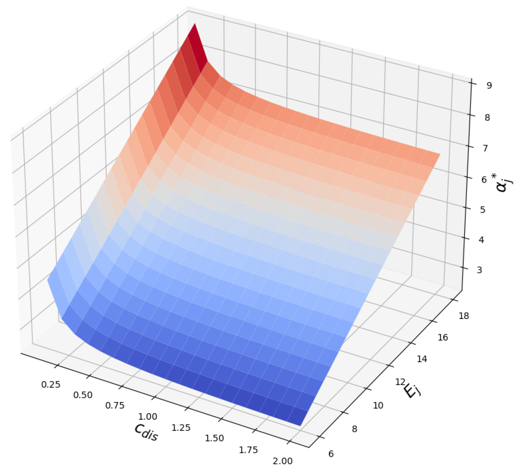
In Figure 3, we analyze the effect of $C_{dis}$ and $E_j$ on the optimal value of EVCF. Since the variables have a proportional relationship with $p^{*}$, it can be confirmed that $p^{*}$ increases with the increment of variables, as depicted in Equation (15). In the equation, we confirm that ${\widehat{p}}^{*}$ is a variable that affects the determination of $p^{*}$. Since $p^{*}$ is affected by changes in $C_{dis}$ and $E_j$, it can be confirmed that the value of $p^{*}$ becomes close to 0 when one of the variables is set close to 0.

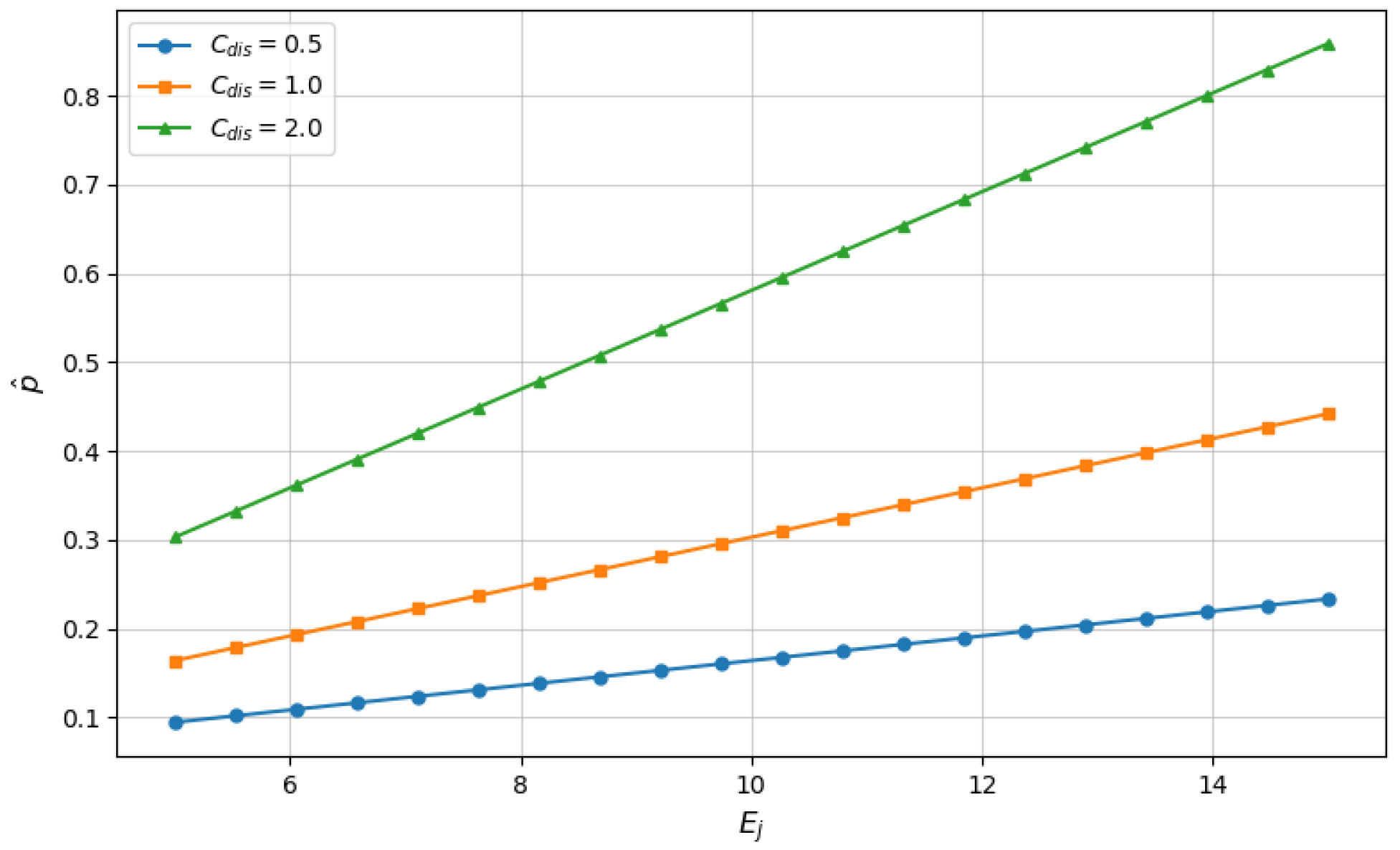
In Figure 4, we could observe that the value of additional charging energy ${\alpha }_j^{*}$ is related with the variation of discomfort factor and conventionally charging energy. As referred to in Equations (10) and (11), it can be seen that EV’s additional charging energy appears in a proportional relationship with ${\displaystyle \frac{1}{C_{dis}}}$. Although the change in $C_{dis}$ increases the incentive provided by EVCF, the direct effect of $C_{dis}$ is greater than the extent of the increment. Therefore, the amount of additional charging energy tends to decrease as the value of $C_{dis}$ increases. Since the values of $E_j$ and $p^{*}$ have a linear proportional relationship, it is confirmed that the values of $E_j$ and ${\alpha }_j$ also have a linear proportional relationship, as shown in the figure.

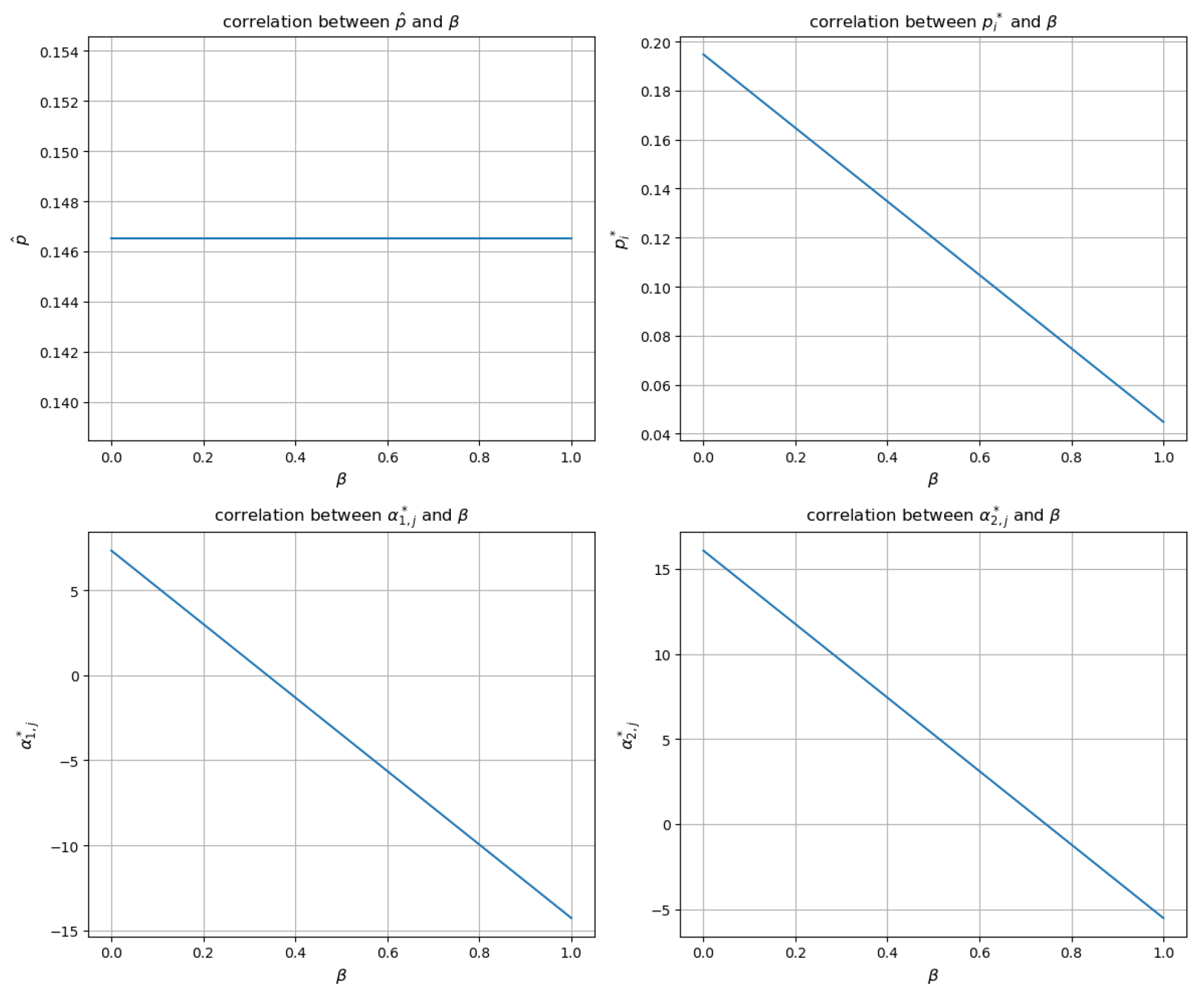
In Figure 5, we analyze the changes in strategies of market participants based on the value of $\beta$, which is an auxiliary variable indicating the cost-sharing ratio between the EVCF and EVs. Since $\beta$ does not directly influence the SO’s strategy decision, the incentive provided by the SO remains unchanged regardless of the change in $\beta$. According to the simulation results, as the value of $\beta$ increases, the incentive $p_i$ provided by the EVCF tends to decrease. As a result, the net utility of EVs decreases, and the optimal additional charging quantity ${\alpha }_j^{*}$ also decreases. Although a higher $\beta$ reduces the direct cost burden on EVs, the decrease in $p_i$ offsets this benefit, leading to a decline in the total profit of EVs and their participation in additional charging. These findings are consistent with the theoretical analysis and Equations (10), (11) and (15).

4.2. Revenue Analysis of Individual Market Participant

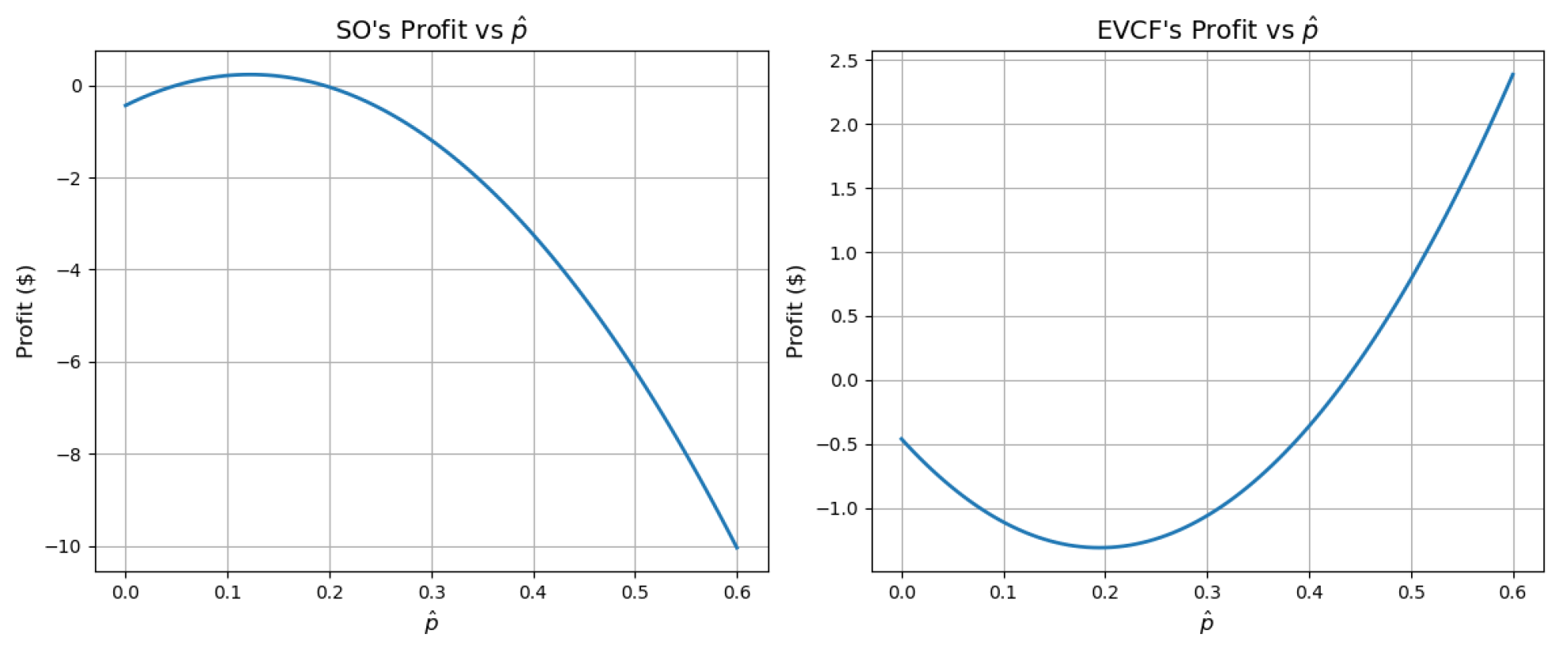
The proposed reverse DR program operates under an environment composed of Stackelberg game theory. In other words, the leader’s decision-making has a significant impact on the strategy decisions of other followers. To analyze this, we set the profit structure of each participant based on the changes in the incentive provided by the SO in this section.

In Figure 6, we analyze the strategy of participants according to the decision-making of SO, which is the leader of the system. From the SO’s perspective, setting the incentive too low makes EVCF and EVs hesitate to participate in the reverse DR program. Conversely, if the incentive is set too high, the issue arises that the SO must bear financial losses while operating the reverse DR program. As shown in the first figure in Figure 6, the SO maximizes its profit when $\widehat{p}$ is set near USD $0.1$.

In the case of EVCF, its profit increases as the incentive $\widehat{p}$ provided by the SO increases. As described in Equation (15), an increase in $\widehat{p}$ leads to a higher profit for the EVCF. Therefore, it is necessary to set $\widehat{p}$ far from USD $0.2$ to effectively implement the reverse DR program. These findings are consistent with the theoretical analysis.

5. Conclusions

In this paper, we propose a scheme to stabilize power supplement in an isolated microgrid through the reverse demand response using electric vehicles and charging facilities. Using the heterogeneous Stackelberg game model, the system operator could determine a proper incentive price to stabilize the power system. In addition, market participants are allowed to choose their own strategies according to their revenue from the demand response program or their discomfort factor based on charging decisions. With the consideration of the net profit of participants in the system, this approach shows that it is possible to maximize the profit of participants while stabilizing energy supplement in an independent energy environment.