
Approaches to Proxy Modeling of Gas Reservoirs

 , and
, and 
Abstract
1. Introduction
- Multifunctional Models (MFMs): Simplified models that employ coarse discretization to accelerate computations;
- Reduced-Order Models (ROMs): Models that reduce system dimensionality while preserving key physical characteristics;
- Traditional Proxy Models (TPMs): Data-driven models based on numerical simulations, requiring minimal understanding of the underlying physical processes;
- Smart Proxy Models (SPMs): Models leveraging machine learning to enhance accuracy by accounting for complex geological features.
- Single Data-Driven Models: These encompass methods based on individual machine learning algorithms, such as multiple linear regression (MLR), support vector regression (SVR), ensemble learning techniques (e.g., random forest and gradient boosting), and neural networks. While these models can yield accurate results, they require meticulous preprocessing of input data to achieve stable performance;
- Combination of Proxy Models: These are developed by utilizing the maximum available data and integrating multiple models into a cohesive solution. Examples include combining neural networks with decision trees or incorporating physical constraints, such as fluid flow equations in porous media, into the model structure.
2. Materials and Methods
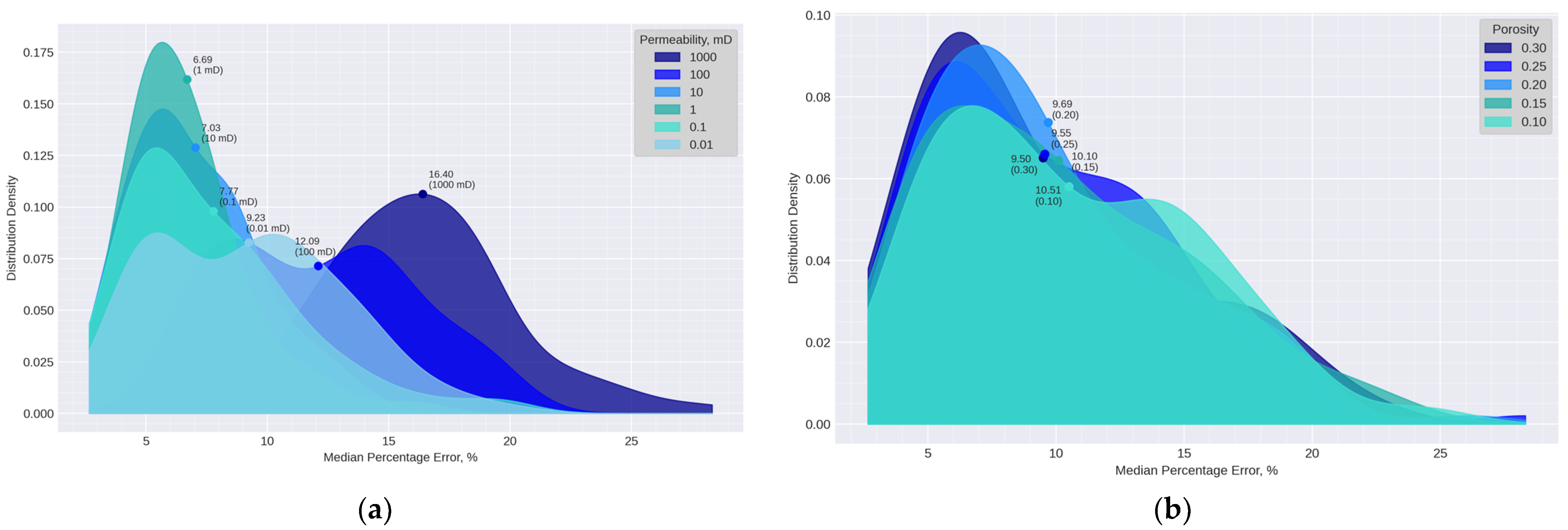
- permeability—0.01 mD; 0.1 mD; 1 mD; 10 mD; 100 mD; 1000 mD;
- porosity—0.10; 0.15; 0.20; 0.25; 0.30;
- initial gas saturation—0.8; 0.9;
- gas viscosity under reservoir conditions—0.01 mPa∙s; 0.03 mPa∙s; 0.05 mPa∙s;
- gas supercompressibility factor (z-factor) under reservoir conditions—0.7; 0.8; 0.9.
3. Results and Discussion
4. Conclusions
Author Contributions
Funding
Data Availability Statement
Conflicts of Interest
Abbreviations
| ANN | Artificial Neural Network |
| BiGRU | Bidirectional Gated Recurrent Unit |
| cDC-GAN | Conditional Deep Convolutional Generative Adversarial Network |
| Conv1D | 1 Dimensional Convolution |
| CRM | Capacitance–Resistance Model |
| DCA | Decline Curve Analysis |
| DHNN | Deep Hybrid Neural Network |
| DNN | Deep Neural Network |
| DPDP | Dual-Porosity Dual-Permeability |
| EOR | Enhanced Oil Recovery |
| FC | Fully Connected |
| FCD | Fracture Conductivity |
| GPR | Gaussian Process Regression |
| HM | Hydrodynamic Model |
| LSTM | Long Short-Term Memory |
| MAE | Mean Absolute Error |
| MAPE | Mean Average Percentage Error |
| MCMC | Markov Chain Monte Carlo |
| MFM | Multifunctional Model |
| MLP | Multilayer Perceptron |
| MLR | Multiple Linear Regression |
| MSE | Mean Squared Error |
| NPV | Net Present Value |
| PIED | Physics-Informed Embedded Decoder |
| PSO | Particle Swarm Optimization |
| ReLU | Rectified Linear Unit |
| RMSE | Root Mean Squared Error |
| ROM | Reduced-Order Model |
| SGD | Stochastic Gradient Descent |
| SPM | Smart Proxy Model |
| SSIM | Structural Similarity Index Measure |
| ST-GNN | Spatio-Temporal Graph Neural Network |
| SVR | Support Vector Regression |
| TPM | Traditional Proxy Model |
Appendix A

| Study Title | Research Objective | Methodology | Advantages | Disadvantages | Application Features |
|---|---|---|---|---|---|
| Data-driven approach for hydrocarbon production forecasting using machine learning techniques [22] | Compare various algorithms, including random forest, gradient boosting, and artificial neural networks, for the evaluation and prediction of daily oil production using data from the Norwegian Volve field as a case study. | Data analysis and preprocessing were performed, including data filtering to address missing values, correction of anomalies, and normalization. Based on Pearson correlation coefficients, key parameters were selected: well pressure, average choke size, volume of injected water, and daily production volume. The tuning of hyperparameters for each machine learning algorithm is described: for random forest, the depth and number of trees were adjusted; for gradient boosting, the learning rate and loss criterion were optimized; and for artificial neural networks (ANNs), activation functions and the number of neurons in hidden layers were selected. The final evaluation of model accuracy was conducted using the metrics MSE, MAE, and the coefficient of determination (R2). | The method does not require detailed physical-mathematical simulation of the reservoir; it effectively handles missing data, well shut-in periods, and complex nonlinear relationships. | The accuracy of the models depends on the quality and quantity of data; challenges arise in tuning hyperparameters; the need for individual algorithm selection for each well is evident, with ANN demonstrating the highest accuracy for one well, while random forest performed best for another. | With a large volume of historical data, machine learning models can complement classical methods of historical analysis and reservoir development modeling to enable rapid forecasting. |
| Machine Learning-Based Production Prediction Model and Its Application in Duvernay Formation [23] | This study examines proxy models based on machine learning for forecasting hydrocarbon production in the Duvernay shale basin, Canada. The research focuses on developing and evaluating the accuracy of three predictive models—MLR, SVR, and GPR—using a range of variables, including geological and technological well parameters. | Based on Grey Relational Analysis and Pearson correlation, key parameters were selected: volume of injected fluid, number of hydraulic fracturing stages, gas saturation, and total organic carbon, which significantly influence cumulative gas and condensate production. During model development, the authors split the dataset into training and testing subsets, employed four-fold cross-validation, and applied Bayesian optimization to tune the hyperparameters of SVR and GPR models, | The GPR model demonstrated the best performance, achieving an R2 of 0.8 for gas and 0.83 for condensate, with RMSE values of 280.54 × 10⁴ m3 and 1884.3 t, respectively, indicating high predictive accuracy. The model is capable of operating with small datasets, making it suitable for fields with limited operational history. | All models require high-quality, preprocessed data to ensure accurate hyperparameter tuning. | The necessity of data preprocessing and the limited applicability to shale reservoirs with similar characteristics. |
| Smart Proxy Modeling of a Fractured Reservoir Model for Production Optimization: Implementation of Metaheuristic Algorithm and Probabilistic Application [24] | Development and demonstration of SPM based on ANN for optimizing hydrocarbon production from fractured reservoirs using metaheuristic algorithms and probabilistic analysis. | Construction of a synthetic model of a fractured reservoir using the dual-porosity dual-permeability (DPDP) method; training of ANN with backpropagation algorithms (SGD, Adam) and the metaheuristic PSO algorithm. | Significant reduction in computational time (50–120 s compared to 160–290 s for numerical modeling); high predictive accuracy (R2 > 0.99); ability to integrate metaheuristic algorithms and probabilistic analysis to enhance forecast reliability. | The model’s performance is limited in scenarios not covered by the training dataset; it is dependent on the quality of the spatio-temporal database. | Requires preliminary data normalization; applicable only to fractured reservoirs with similar characteristics. |
| Application of Machine Learning Method of Data-Driven Deep Learning Model to Predict Well Production Rate in the Shale Gas Reservoirs [25] | Development and validation of a proxy model based on machine learning methods (DNN) for forecasting cumulative gas production from shale reservoirs, using real data from the Montney Formation, Canada. | A deep neural network approach based on a multilayer perceptron was employed. Preliminary data analysis and variable importance analysis were conducted using Random Forest, Gradient Boosting Machine, and XGBoost. Dimensionality reduction was performed via Principal Component Analysis, and hyperparameter optimization (including one-hot encoding, ReLU activation, dropout, and others) was carried out based on data from 1150 wells. | Significant reduction in computational time compared to numerical modeling; high predictive accuracy (MAPE up to 22.14%); ability to integrate categorical and numerical data for the analysis of shale reservoirs. | Limited applicability in the absence of sufficient data volume or changes in geological conditions; dependence on the quality of input data and the accuracy of its preprocessing; lack of consideration for time-series data. | Requires thorough data preprocessing (normalization, outlier removal); applicable to horizontal wells with multistage hydraulic fracturing; recommended to perform sensitivity analysis of hyperparameters for model adaptation. |
| Forecasting oil production in unconventional reservoirs using long short term memory network coupled support vector regression method: A case study [26] | Development of a hybrid LSTM-SVR model for forecasting oil production in low-permeability reservoirs, incorporating time-series and operational parameters, and enhancing predictive accuracy through residual connections. | A hybrid LSTM-SVR model was employed: LSTM for initial production forecasting, SVR for predicting residuals, followed by correction of the LSTM forecast; data from the Ma-18 block of the Xinjiang field (two wells, 1182 and 1186 data points) were used; data preprocessing included Z-score normalization and imputation of missing values. | High predictive accuracy (RMSE up to 0.94); incorporation of time-series and operational parameters; effective residual correction via SVR improves forecasting with limited data. | Prediction error increases with longer forecasting horizons; high sensitivity to abrupt changes in operational parameters; complexity in hyperparameter tuning. | Requires thorough data preprocessing (normalization, imputation of missing values); applicable to low-permeability reservoirs with significant intra-reservoir heterogeneity. |
| Predicting field production rates for waterflooding using a machine learning-based proxy model [27] | Development and implementation of a proxy model based on a conditional deep convolutional generative adversarial network (cDC-GAN) for rapid calculation of dynamic fluid distribution and forecasting production volumes during water injection as a secondary oil recovery technique. | A cDC-GAN model was employed, comprising generative and discriminative components. Input data included reservoir properties (permeability distribution) and forecast time, with water saturation as the output; data were generated using geostatistical methods and the numerical simulator. Production rate calculations were based on the material balance principle. | Significant reduction in computational costs compared to numerical modeling; high predictive accuracy for water saturation and total fluid production (SSIM ≥ 0.96); ability to use raw input data without preliminary feature processing. | Limited extrapolation capability (error increases after three years); inability to separate production rates by individual wells; inability to adapt to abrupt changes, such as water breakthrough. | Applicable to 2D models for waterflooding; requires large datasets for training; recommended to incorporate additional geological and operational parameters to enhance accuracy. |
| Highly accurate oil production forecasting under adjustable policy by a physical approximation network [28] | Development of a neural network model for accurate forecasting of oil production, accounting for variable field development strategies, using a dynamic graph-based approach that incorporates physical processes occurring in the reservoir. | A Double-channel Heterogeneous Dynamical Graph network model was proposed; input data comprised historical production data, geological parameters, and control variables (injection and production fluid rates); the graph structure included wells as nodes and reservoir conditions between wells as edges; training was conducted on synthetic Egg and Brugge datasets (2400 days), validation on 10 days, and forecasting for 600 days, with comparisons against LSTM and the Eclipse simulator. | High forecasting accuracy incorporating physical processes (MSE ~ 1.15 × 10⁻⁵ for Egg, 2.35 × 10⁻⁵ for Brugge); significant reduction in computational time; automated training without manual tuning; ability to adapt to changing field development strategies. | Tested only on sandstone reservoirs, with applicability to carbonate reservoirs unconfirmed; reduced accuracy for forecasts beyond 600 days; sensitivity to insufficient reservoir energy. | Requires significant modifications to historical data for training; accounts for spatio-temporal dependencies. |
| Study Title | Research Objective | Methodology | Advantages | Disadvantages | Application Features |
|---|---|---|---|---|---|
| CO2 EOR Performance Evaluation in an Unconventional Reservoir through Mechanistic Constrained Proxy Modeling [29] | Evaluation of CO2 injection efficiency in unconventional reservoirs using a deep neural network to develop proxy models for forecasting oil production, incorporating reservoir characteristics and hydraulic fracturing parameters. | A 3D model with dual porosity and hydraulic fracturing was constructed; physical constraints were incorporated using data obtained from comprehensive numerical modeling; input data included reservoir pressure, matrix permeability, fracture permeability, and FCD; output data consisted of the oil recovery factor; the dataset comprised 396 simulations; the DNN model featured 10 hidden layers, over 1500 neurons, ReLU activation, Adam optimizer, and k-fold cross-validation; forecasts were made for 5 and 10 years. | High forecasting accuracy (R2 > 0.95); rapid generation of proxy models; reduced computational time compared to traditional simulations. | Limited accuracy at high fracture permeability and FCD values (underestimation); applicability restricted to unconventional reservoirs with low permeability; requires a large volume of data for training. | Applicable to unconventional reservoirs with low permeability; optimal for medium pressures; requires data normalization; sensitive to the quality of input data. |
| A Physics-Informed Neural Network Approach for Surrogating a Numerical Simulation of Fractured Horizontal Well Production Prediction [30] | Development of a PIED neural network to replace numerical simulations in forecasting production from horizontal wells with unequally spaced intersecting hydraulic fractures, incorporating physical constraints. | A PIED architecture based on Seq2Seq (LSTM-LSTM) was developed; input data included fracture length, permeability, and dip angle; the dataset comprised 500 simulations (10 fractures); the decoder’s intermediate input was production time; comparisons were made with MLP and LSTM-Attention-LSTM models. | High accuracy (MAE 168.81, error 2.7%); ability to operate with small datasets (500 samples over 3 days); incorporation of physical constraints; reduction in error accumulation; effective handling of high-dimensional data (30 variables). | Limited incorporation of physical information (only fracture geometry and production time); unverified applicability for a large number of fractures (>10); potential overfitting with increased data dimensionality. | Applicable to horizontal wells with intersecting fractures; requires data normalization; optimal for sequential data; sensitive to the order of fractures. |
| A physics-constrained long-term production prediction method for multiple fractured wells using deep learning [31] | Long-term forecasting of oil production from wells with multiple hydraulic fracturing operations under conditions of limited data and complex geological structures. | Development of a hybrid BiGRU-DHNN model combining bidirectional gated recurrent unit neural networks for time-series production analysis and a deep hybrid neural network to incorporate physical constraints; input data included well depth, horizontal section length, number of hydraulic fracturing stages, sand volume, fluid volume, gamma-ray logging, acoustic logging, reservoir resistivity, tubing pressure, choke sizes, and oil production. | Reduced forecasting errors: RMSE and MAE values of 5.4 and 4.2, respectively (compared to 10–15 for models without constraints), with R2 = 0.46 (compared to 0.2–0.3 for models without constraints); ability to capture complex relationships between production and system input parameters. | Error accumulation in iterative strategies: error increases with longer forecasting horizons (e.g., high accuracy in the first year, but deviations reach 20–30% by the third year); dependence on data volume (requires at least 11 wells for training). | Requires data normalization; applicable to wells with known hydraulic fracturing parameters. |
| A Physics-Informed Spatial-Temporal Neural Network for Reservoir Simulation and Uncertainty Quantification [32] | Modeling of reservoir development and quantitative assessment of uncertainties in oil production in heterogeneous reservoirs. | The PI-STNN model integrates a deep convolutional encoder–decoder for processing spatial data and a convolutional LSTM (ConvLSTM) to account for temporal dependencies; input data include permeability, porosity, pressure (initial reservoir, bottomhole, and average), oil viscosity, oil density, grid dimensions, time step, and production; physical constraints are incorporated by embedding partial differential equations describing fluid filtration in porous media into the loss function, with the Pisman formula used as the governing equation. | High accuracy: median R2 values range from ~0.95 (10 fractures) to ~0.9 (62 fractures), with a range of 0.85–1.0; accelerated computations, with 12,008.9 s compared to 237,504.2 s for traditional simulators. | Limited to single-phase flow; complexity in adapting to multiphase and multicomponent systems. | Applicable to heterogeneous reservoirs with fractures; effective for uncertainty analysis and NPV calculations. |
References
- Bret-Rouzaut, N. Economics of Oil and Gas Production. In The Palgrave Handbook of International Energy Economics; Hafner, M., Luciani, G., Eds.; Palgrave Macmillan: Cham, Switzerland, 2022; pp. 3–24. ISBN 978-3-030-86883-3. [Google Scholar]
- Werneck, L.F.; Heringer, J.D.d.S.; de Souza, G.; Souto, H.P.A. Numerical Simulation of Non-Isothermal Flow in Oil Reservoirs Using a Coprocessor and the OpenMP. Comput. Appl. Math. 2023, 42, 365. [Google Scholar] [CrossRef]
- Ng, C.S.W.; Nait Amar, M.; Jahanbani Ghahfarokhi, A.; Imsland, L.S. A Survey on the Application of Machine Learning and Metaheuristic Algorithms for Intelligent Proxy Modeling in Reservoir Simulation. Comput. Chem. Eng. 2023, 170, 108107. [Google Scholar] [CrossRef]
- Bahrami, P.; Sahari Moghaddam, F.; James, L.A. A Review of Proxy Modeling Highlighting Applications for Reservoir Engineering. Energies 2022, 15, 5247. [Google Scholar] [CrossRef]
- Cao, C.; Jia, P.; Cheng, L.; Jin, Q.; Qi, S. A review on application of data-driven models in hydrocarbon production forecast. J. Pet. Sci. Eng. 2022, 212, 110296. [Google Scholar] [CrossRef]
- Liang, H.-B.; Zhang, L.-H.; Zhao, Y.-L.; Zhang, B.-N.; Chang, C.; Chen, M.; Bai, M.-X. Empirical methods of decline-curve analysis for shale gas reservoirs: Review, evaluation, and application. J. Nat. Gas Sci. Eng. 2020, 83, 103531. [Google Scholar] [CrossRef]
- Montgomery, J.B.; Raymond, S.J.; O’Sullivan, F.M.; Williams, J.R. Shale gas production forecasting is an ill-posed inverse problem and requires regularization. Upstream Oil Gas Technol. 2020, 5, 100022. [Google Scholar] [CrossRef]
- Holanda, R.W.d.; Gildin, E.; Jensen, J.L.; Lake, L.W.; Kabir, C.S. A State-of-the-Art Literature Review on Capacitance Resistance Models for Reservoir Characterization and Performance Forecasting. Energies 2018, 11, 3368. [Google Scholar] [CrossRef]
- Yudin, E.V.; Markov, N.S.; Kotezhekov, V.S.; Kraeva, S.O.; Makhnov, A.V.; Trubnikov, N.P.; Gorbushin, L.A. Efficiency of Using a Proxy Model for Modeling of Reservoir Pressure. In Proceedings of the SPE Russian Petroleum Technology Conference, Virtual, 12–15 October 2021. [Google Scholar] [CrossRef]
- Gross, H. History Matching Production Data Using Streamlines and Geostatistics. Ph.D. Thesis, Stanford University, Stanford, CA, USA, 2006. [Google Scholar]
- Thiele, M.R.; Fenwick, D.H.; Batycky, R.P. Streamline-Assisted History Matching. In Proceedings of the 9th International Forum on Reservoir Simulation, Abu Dhabi, United Arab Emirates, 9–13 December 2007. [Google Scholar]
- Goodwin, N. Bridging the Gap Between Deterministic and Probabilistic Uncertainty Quantification Using Advanced Proxy Based Methods. In Proceedings of the SPE Reservoir Simulation Symposium, Houston, TX, USA, 23–25 February 2015. [Google Scholar] [CrossRef]
- Wu, Z.; Pan, S.; Chen, F.; Long, G.; Zhang, C.; Yu, P.S. A Comprehensive Survey on Graph Neural Networks. IEEE Trans. Neural Netw. Learn. Syst. 2021, 32, 4–24. [Google Scholar] [CrossRef]
- Hochreiter, S.; Schmidhuber, J. Long Short-Term Memory. Neural Comput. 1997, 9, 1735–1780. [Google Scholar] [CrossRef]
- LeCun, Y.; Bottou, L.; Bengio, Y.; Haffner, P. Gradient-Based Learning Applied to Document Recognition. Proc. IEEE 1998, 86, 2278–2324. [Google Scholar] [CrossRef]
- Kipf, T.N.; Welling, M. Semi-Supervised Classification with Graph Convolutional Networks. In Proceedings of the International Conference on Learning Representations (ICLR), Toulon, France, 24–26 April 2017; pp. 1–14. [Google Scholar] [CrossRef]
- Rosenblatt, F. The Perceptron: A Probabilistic Model for Information Storage and Organization in the Brain. Psychol. Rev. 1958, 65, 386–408. [Google Scholar] [CrossRef]
- Vaferi, B.; Eslamloueyan, R.; Ghaffarian, N. Hydrocarbon Reservoir Model Detection from Pressure Transient Data Using Coupled Artificial Neural Network—Wavelet Transform Approach. Appl. Soft Comput. 2016, 47, 63–75. [Google Scholar] [CrossRef]
- Ngoc, K.M.; Lee, M. Forecasting COVID-19 confirmed cases in South Korea using Spatio-Temporal Graph Neural Networks. Int. J. Contents 2021, 17, 1–14. [Google Scholar] [CrossRef]
- Xu, L.; Yuxuan, L.; Chao, H.; Hengchang, H.; Yushi, C.; Bryan, H.; Roger, Z. Do We Really Need Graph Neural Networks for Traffic Forecasting? arXiv 2023, arXiv:2301.12603. [Google Scholar] [CrossRef]
- Rock Flow Dynamics. tNavigator, Version 23.1; Rock Flow Dynamics: Moscow, Russia, 2023. Available online: https://rfdyn.com (accessed on 12 April 2023).
- Chahar, J.; Verma, J.; Vyas, D.; Goyal, M. Data-driven approach for hydrocarbon production forecasting using machine learning techniques. J. Pet. Sci. Eng. 2022, 217, 110757. [Google Scholar] [CrossRef]
- Guo, Z.; Wang, H.; Kong, X.; Shen, L.; Jia, Y. Machine Learning-Based Production Prediction Model and Its Application in Duvernay Formation. Energies 2021, 14, 5509. [Google Scholar] [CrossRef]
- Ng, C.S.W.; Ghahfarokhi, A.J.; Amar, M.N.; Torsæter, O. Smart Proxy Modeling of a Fractured Reservoir Model for Production Optimization: Implementation of Metaheuristic Algorithm and Probabilistic Application. Nat. Resour. Res. 2021, 30, 2431–2462. [Google Scholar] [CrossRef]
- Dongkwon, H.; Sunil, K. Application of Machine Learning Method of Data-Driven Deep Learning Model to Predict Well Production Rate in the Shale Gas Reservoirs. Energies 2021, 14, 3629. [Google Scholar] [CrossRef]
- Wen, S.; Wei, B.; You, J.; He, Y.; Xin, J.; Varfolomeev, M.A. Forecasting oil production in unconventional reservoirs using long short term memory network coupled support vector regression method: A case study. Petroleum 2023, 9, 647–657. [Google Scholar] [CrossRef]
- Zhong, Z.; Sun, A.Y.; Wang, Y.; Ren, B. Predicting field production rates for waterflooding using a machine learning-based proxy model. J. Pet. Sci. Eng. 2020, 194, 107574. [Google Scholar] [CrossRef]
- Wang, H.; Zhang, K.; Deng, X.; Cui, S.; Ma, X.; Wang, Z.; Qi, J.; Wang, J.; Yao, C.; Zhang, L.; et al. Highly accurate oil production forecasting under adjustable policy by a physical approximation network. Energy Rep. 2022, 8, 14396–14415. [Google Scholar] [CrossRef]
- Syed, F.I.; Muther, T.; Dahaghi, A.K.; Neghabhan, S. CO2 EOR Performance Evaluation in an Unconventional Reservoir through Mechanistic Constrained Proxy Modeling. Fuel 2022, 310, 122390. [Google Scholar] [CrossRef]
- Jin, T.; Xia, Y.; Jiang, H. A Physics-Informed Neural Network Approach for Surrogating a Numerical Simulation of Fractured Horizontal Well Production Prediction. Energies 2023, 16, 7948. [Google Scholar] [CrossRef]
- Li, X.; Ma, X.; Xiao, F.; Xiao, C.; Wang, F.; Zhang, S. A physics-constrained long-term production prediction method for multiple fractured wells using deep learning. J. Pet. Sci. Eng. 2022, 217, 110844. [Google Scholar] [CrossRef]
- Bi, J.; Li, J.; Wu, K.; Chen, Z.; Chen, S.; Jiang, L.; Feng, D.; Deng, P. A Physics-Informed Spatial-Temporal Neural Network for Reservoir Simulation and Uncertainty Quantification. SPE J. 2024, 29, 2026–2043. [Google Scholar] [CrossRef]


| Dataset | Data Source | Entity | Distribution |
|---|---|---|---|
| Distantly located wells | Results of hydrodynamic simulator calculations on an artificial HM. | Two wells located 15 km apart (homogeneous geological properties). | • training set—15,120 simulations; • validation set—540 simulations; • test set—540 simulations. |
| Closely located wells | Results of hydrodynamic simulator calculations on an artificial HM. | Two wells located 1 km apart (homogeneous geological properties). | • training set—15,120 simulations; • validation set—540 simulations; • test set—540 simulations. |
| HM of the field | Results of hydrodynamic simulator calculations on the field’s HM. | Irregular grid of 8 wells (heterogeneous geological properties) penetrating a single hydrodynamically connected system. | • training set—23 simulations; • validation set—1 simulation; • test set—1 simulation. |
| Real data from sensors | Data from field sensors and devices. | Irregular grid of 86 wells (heterogeneous geological properties) penetrating a single hydrodynamically connected system. | • training set—89 measurements; • validation set—8 measurements; • test set—21 measurements. |
| Dataset | Sequence Length | Learning Rate, 10−4 | Weight Decay, 10−5 |
|---|---|---|---|
| Distantly located wells | 20 | 3 | 1 |
| Closely located wells | 20 | 3 | 1 |
| HM of the field | 7 | 5 | 10 |
| Real data from sensors | 7 | 5 | 1 |
| Dataset | Median AE, 103 m3 | Max AE, 103 m3 | RMSE, 103 m3 | Median APE, % | Max APE, % |
|---|---|---|---|---|---|
| HM of the field | 96 | 2246 | 272 | 1.8 | 30.3 |
| Real data from sensors | 819 | 15,942 | 1190 | 9.8 | 345 |
| Dataset | ST-GNN Speedup Relative to HM Without Training | ST-GNN Speedup Relative to HM with Training |
|---|---|---|
| Distantly located wells | 20,080 | 4.8 |
| Closely located wells | 20,830 | 1.7 |
| HM of the field | 23,900 | 6.6 |
| Real data from sensors | – | – |
Disclaimer/Publisher’s Note: The statements, opinions and data contained in all publications are solely those of the individual author(s) and contributor(s) and not of MDPI and/or the editor(s). MDPI and/or the editor(s) disclaim responsibility for any injury to people or property resulting from any ideas, methods, instructions or products referred to in the content. |
© 2025 by the authors. Licensee MDPI, Basel, Switzerland. This article is an open access article distributed under the terms and conditions of the Creative Commons Attribution (CC BY) license (https://creativecommons.org/licenses/by/4.0/).
Share and Cite
Perepelkin, A.; Sharifov, A.; Titov, D.; Shandrygolov, Z.; Derkach, D.; Islamov, S. Approaches to Proxy Modeling of Gas Reservoirs. Energies 2025, 18, 3881. https://doi.org/10.3390/en18143881
Perepelkin A, Sharifov A, Titov D, Shandrygolov Z, Derkach D, Islamov S. Approaches to Proxy Modeling of Gas Reservoirs. Energies. 2025; 18(14):3881. https://doi.org/10.3390/en18143881
Chicago/Turabian StylePerepelkin, Alexander, Anar Sharifov, Daniil Titov, Zakhar Shandrygolov, Denis Derkach, and Shamil Islamov. 2025. "Approaches to Proxy Modeling of Gas Reservoirs" Energies 18, no. 14: 3881. https://doi.org/10.3390/en18143881
APA StylePerepelkin, A., Sharifov, A., Titov, D., Shandrygolov, Z., Derkach, D., & Islamov, S. (2025). Approaches to Proxy Modeling of Gas Reservoirs. Energies, 18(14), 3881. https://doi.org/10.3390/en18143881