A Mechanical Fault Diagnosis Method for On-Load Tap Changers Based on GOA-Optimized FMD and Transformer

Abstract

Mechanical failures frequently occur in On-Load Tap Changers (OLTCs) during operation, potentially compromising the reliability and stability of power systems. The goal of this study is to develop an intelligent and accurate diagnostic approach for OLTC mechanical fault identification, particularly under the challenge of non-stationary vibration signals. To achieve this, a novel hybrid method is proposed that integrates the Gazelle Optimization Algorithm (GOA), Feature Mode Decomposition (FMD), and a Transformer-based classification model. Specifically, GOA is employed to automatically optimize key FMD parameters, including the number of filters (K), filter length (L), and number of decomposition modes (N), enabling high-resolution signal decomposition. From the resulting intrinsic mode functions (IMFs), statistical time domain features—peak factor, impulse factor, waveform factor, and clearance factor—are extracted to form feature vectors. After feature extraction, the resulting vectors are utilized by a Transformer to classify fault types. Benchmark comparisons with other decomposition and learning approaches highlight the enhanced performance of the proposed framework. The model achieves a 95.83% classification accuracy on the test set and an average of 96.7% under five-fold cross-validation, demonstrating excellent accuracy and generalization. What distinguishes this research is its incorporation of a GOA–FMD and a Transformer-based attention mechanism for pattern recognition into a unified and efficient diagnostic framework. With its high effectiveness and adaptability, the proposed framework shows great promise for real-world applications in the smart fault monitoring of power systems.

1. Introduction

The On-Load Tap Changer (OLTC) plays a fundamental role in maintaining voltage stability by allowing tap transitions under load without power interruptions [1,2,3]. The performance and reliability of OLTCs are essential to the overall stability and voltage control of power systems, directly impacting the quality and continuity of electrical service delivery. According to statistical analyses, OLTC-related failures constitute over 20% of total transformer malfunctions, with mechanical issues comprising more than 70% of these cases [4,5,6]. These statistics indicate that OLTC mechanical faults rank among the most frequent and disruptive failure types in power transformers. Mechanical faults can lead to abnormal switching behavior, prolonged tap transition time, contact overheating, or even permanent failure. These faults often result in voltage fluctuations, power quality deterioration, and in severe cases, forced transformer shutdowns or grid instability [7]. As a result, the efficient and precise extraction of vibration signal features for the accurate assessment of equipment condition and fault diagnosis has emerged as a central concern in recent research.

OLTC vibration signals encapsulate abundant information related to mechanical operating states and fault characteristics, effectively reflecting the condition of mechanical components. Xu et al. employed time–frequency analysis in conjunction with signal decomposition techniques to extract diagnostic features from vibration signals [8]. The Empirical Mode Decomposition (EMD) algorithm decomposes the entire signal during OLTC tap transitions to obtain time domain energy features by constructing envelopes based on local extrema and interpolating intrinsic mode functions (IMFs). However, due to its reliance on extrema and symmetric envelopes, EMD is prone to mode mixing and boundary artifacts, which can lead to ambiguous decomposition results and the potential omission of critical information [9]. To address these limitations, Liu et al. introduced the Variational Mode Decomposition (VMD) technique for OLTC fault diagnosis [10]. Theoretically, VMD separates the signal into multiple narrowband components with a primary emphasis on frequency domain characteristics [11,12]. Nevertheless, it fails to adequately capture the impulsive and periodic features inherent in mechanical faults. A recent study introduced (FMD), a technique designed to utilize adaptive filters with limited-bandwidth impulse responses to decompose signals into modal components that exhibit minimal correlation with the original signal [13]. FMD retains both periodic and transient signal features and demonstrates notable robustness under noise interference. However, its performance is highly sensitive to parameter configuration, which has a substantial impact on the quality of decomposition. The Gazelle Optimization Algorithm (GOA), a recently developed swarm intelligence technique, offers strong global search capabilities and high adaptability, making it particularly effective for solving complex, multimodal, and high-dimensional optimization tasks [14]. While FMD is capable of decomposing signals into IMFs that capture relevant fault information, its efficacy is heavily dependent on optimal parameter settings [15]. To address this, the present study integrates GOA to automatically optimize FMD parameters, thereby enhancing decomposition accuracy. Precise signal decomposition serves as the foundation for reliable feature extraction and classification, and is essential for realizing the intelligent fault diagnosis of OLTC mechanical systems. To illustrate the strengths and limitations of existing signal decomposition approaches in OLTC vibration analysis,

Table 1. Comparison of representative signal decomposition methods for OLTC vibration analysis.

Method	Reference	Advantages	Limitations
EMD	Xu et al. [8,9]	Simple implementation; captures nonlinear and non-stationary signals	Mode mixing; boundary effect; sensitive to extrema; may miss key features
VMD	Liu et al. [10,11,12]	Theoretically sound; decomposes into narrowband modes in frequency domain	Inadequate in capturing transient/impulse features of mechanical faults
FMD	Miao et al. [13,15]	Retains both periodic and impulsive features; noise-resilient	Highly sensitive to parameter settings; requires fine-tuned configuration
GOA-FMD	This study	Automatically optimized parameters via GOA; adaptive and accurate decomposition	None reported in this study

summarizes a comparative overview of the methods used in previous studies and the proposed GOA-FMD approach.

In the domain of OLTC fault diagnosis, achieving high-precision fault classification is essential for enhancing diagnostic accuracy and ensuring model generalization. Several classic machine learning techniques—including Support Vector Machines (SVMs), K-Nearest Neighbors (KNN), and Random Forests (RFs)—offer a certain level of diagnostic capability [16,17,18]. However, these methods typically rely on manually engineered features and exhibit limited adaptability and scalability in complex or dynamic environments. By contrast, deep learning techniques leverage neural networks for automatic feature extraction, thereby improving classification performance [19]. As a type of dense neural network with forward-only signal propagation, the Multilayer Perceptron (MLP) is typically effective for processing data with limited complexity and uniform input dimensions. Nonetheless, its dependence on handcrafted features and its inherent limitations in handling high-dimensional, nonlinear, or unstructured data can compromise its generalization ability [20]. In recent years, the Transformer architecture, underpinned by attention mechanisms, has emerged as a powerful model for feature representation [21,22,23]. Its capacity to capture long-range dependencies and integrate multi-source feature interactions makes it highly effective for complex classification tasks involving multiple feature dimensions. To highlight the advantages of the proposed Transformer-based classifier,

Table 2. Comparison of classification models for OLTC mechanical fault diagnosis.

Method	Model Type	Advantages	Limitations
SVM [16]	Machine Learning	Effective in small datasets; good at binary classification	Requires manual feature extraction; poor scalability in high-dimensional data
KNN [17]	Machine Learning	Simple implementation; intuitive	Sensitive to noise; high computational cost for large datasets
RF [18]	Machine Learning	Handles nonlinearity; robust to overfitting	Feature engineering needed; lacks interpretability
MLP [20]	Deep Learning	Learns nonlinear mappings; handles fixed-size input vectors	Relies on handcrafted features; poor at capturing temporal/spatial structure
Transformer [21,22,23]	Deep Learning	Captures long-range dependencies; automatic feature integration; highly generalizable	High training cost

provides a comparative summary of the common classification methods used in OLTC fault diagnosis, outlining their strengths and limitations in terms of feature extraction, generalization, and adaptability.

To address the limitations in diagnostic accuracy caused by incomplete feature extraction from OLTC mechanical vibration signals, this paper presents an adaptive feature extraction scheme that integrates FMD with parameter tuning performed via the GOA. To improve decomposition accuracy, GOA is employed to fine-tune essential FMD parameters, such as filter count (K), filter length (L), and the number of modes (N). The obtained Intrinsic Mode Functions (IMFs) undergo detailed inspection across time, frequency, and joint time–frequency domains to ensure thorough signal characterization. On this basis, a Transformer-based fault classification model is developed to leverage attention mechanisms for effective feature learning. An experimental platform is subsequently established to simulate OLTC mechanical fault conditions. Three representative fault types are designed: (1) gear jamming in drive shaft; (2) loose screw in drive shaft; (3) arc plate looseness and contact wear. Fault identification is conducted using the proposed feature extraction method in conjunction with the Transformer classifier. To validate the proposed approach, comparative experiments are performed against alternative signal decomposition and classification techniques. The results confirm that the proposed approach achieves a high diagnostic precision and strong resilience under varying operating conditions.

2. GOA-FMD-Based Vibration Signal Feature Extraction and Fault Diagnosis Method

2.1. Principles and Characteristics of FMD

When the OLTC operates under mechanical fault scenarios, its vibration responses embed rich diagnostic characteristics that reflect distinct fault behaviors. FMD, initially designed for diagnosing faults in rotating equipment, is adapted in this study to suit OLTC diagnostic requirements and aims to iteratively extract modal components that carry diagnostic features by applying a sequence of limited-bandwidth impulse response filters. 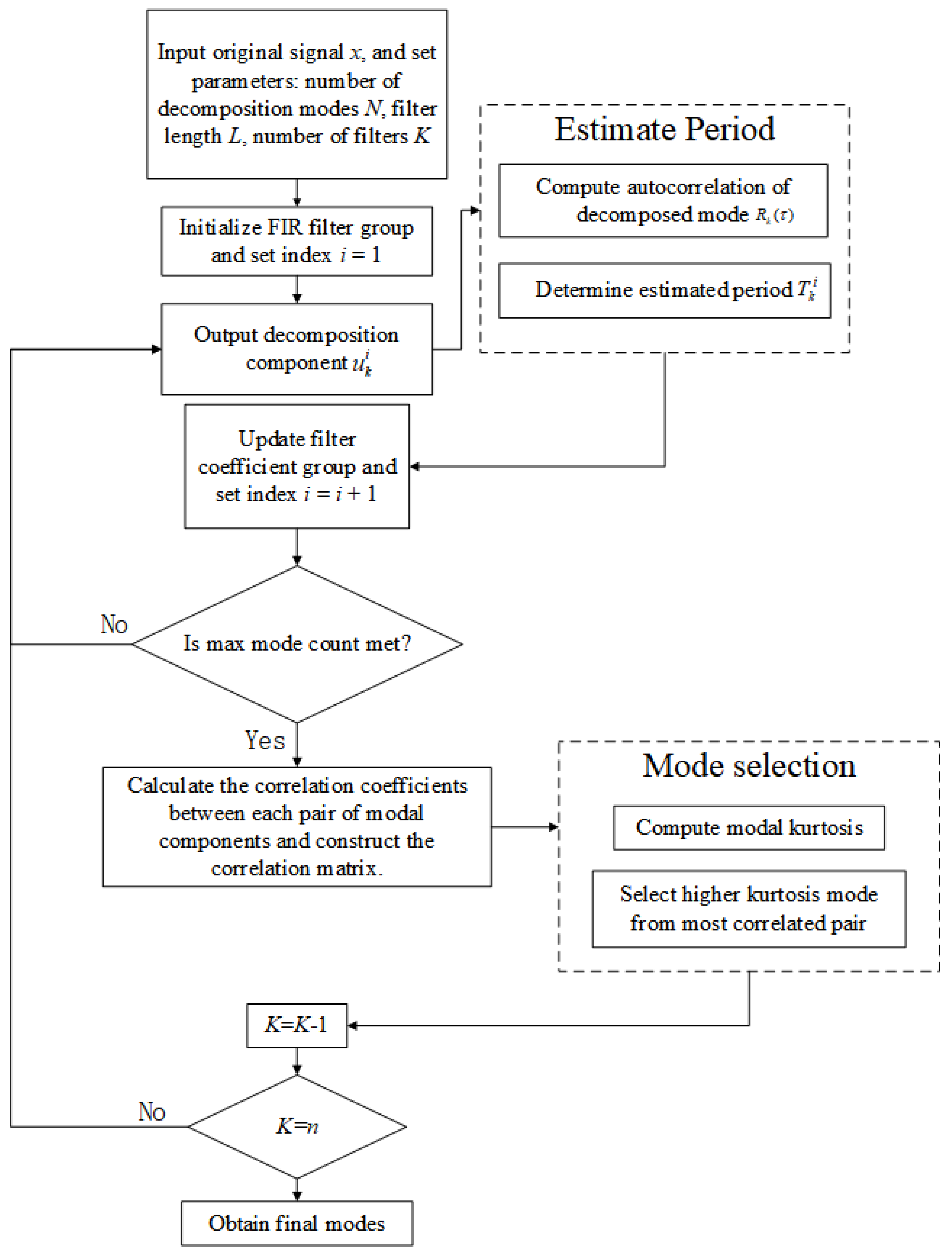This approach suppresses irrelevant components while improving the separability and interpretability of fault-relevant features [13]. FMD has exhibited strong adaptability and reliability in the context of OLTC fault diagnosis. The fundamental procedure of FMD signal decomposition is summarized as follows:

• Provide the input signal x, define the filter length T, and initialize the iteration index i = 1. Specify the total number of filters K, then perform the initial modal decomposition based on the current parameters.
• Output the decomposition components $u_k^i=x*f_k^i$, where $k=1,2,3\dots ,K$, ‘$*$’ indicates convolution, and f_k represents the k-th finite impulse response (FIR) filter.
• Utilize the original signal x, the decomposed component $u_k^i$, and the calculated period $T_k^i$ to update filter coefficients. $T_k^i$ is identified as the time lag at which the autocorrelation function $R_k(\tau )$ reaches its peak after the zero crossing event. The autocorrelation is calculated as follows:

  $$R_k(\tau )={\displaystyle \sum u_k^i[t]u_k^i[t+\tau ]}$$

  (1)

  where τ denotes the time delay and t is the time index of the signal. Finally, the iteration index is updated as i = i + 1.
• Continue to Step 2 if the predefined iteration limit has not been met; otherwise, move forward to Step 5.
• Compute the correlation coefficient $C{C}_{pq}$ for every pairwise combination of modal components $u_p$ and $u_q$, using the formula below.

  $$C{C}_{pq}={\displaystyle \frac{{\displaystyle \sum (u_p(t)-{\overline{u}}_p)(u_q(t)-{\overline{u}}_q)}}{\sqrt{{\displaystyle \sum {(u_p(t)-{\overline{u}}_p)}^2}}\cdot \sqrt{{\displaystyle \sum {(u_q(t)-{\overline{u}}_q)}^2}}}}$$

  (2)

  where $\overline{u}$ denotes the mean value of the corresponding modal component. Form a $K\times K$ matrix $C{C}_{(K\times K)}$ containing the pairwise correlation coefficients, and identify the modal component with the lowest correlation—i.e., the one associated with the smallest maximum value in its corresponding row (or column) of $C{C}_{(K\times K)}$.
• Compute the periodic correlation degree CK of each modal component u_k using the following formula:

  $$CK(u_k)={\displaystyle \frac{{\displaystyle \sum {\left(\prod _{m=0}^M{u}_k(t-m{T}_k)\right)}^2}}{{\displaystyle \sum u_k{(t)}^2}}}$$

  (3)

  where M is the correlation order, representing the number of periodic points used in the computation of CK. The mode exhibiting the highest degree of periodic correlation is designated as the final extracted component. Then, increment the mode index: K = K + 1.
• Assess whether the total number of extracted components K has attained the set value N. If this requirement is met, continue to Step 8; otherwise, revert to Step 2 and repeat the decomposition.

A schematic representation of the FMD algorithm is provided in Figure 1.

The performance of FMD in analyzing OLTC vibration signals is highly sensitive to the parameter settings, which significantly affect the decomposition results [24,25,26]. A short filter length L may result in under-decomposition, whereas an excessively long filter may introduce significant noise into the decomposed components. Similarly, setting too few number of modes N may cause the loss of critical features, while too many modes may result in redundant information [15,27]. The number of filters K also plays a crucial role—if improperly chosen, it can either reduce the decomposition resolution or increase computational complexity unnecessarily [28]. Since FMD lacks an inherent mechanism for adaptive parameter selection, optimization algorithms are required to perform parameter tuning and ensure the accurate extraction of critical fault features from OLTC vibration signals.

2.2. FMD Parameter Optimization via GOA

GOA draws inspiration from natural predator–prey dynamics and operates within the framework of swarm intelligence techniques [14,29]. The optimization process begins with the random initialization of a gazelle population, which serves as candidate solutions in the search process. The population is represented by an $n\times d$ position matrix X, where n denotes the number of agents and d is the dimensionality of the problem. Each row in X denotes the position vector of a candidate gazelle in the search domain. Gazelle population positions are defined by the position matrix X as shown in Equation (4) as follows:

$$X=\left[\begin{array}{ccccc}{x}_{1,1}& x_{1,2}& \dots & x_{1,d-1}& x_{1,d}\\ x_{2,1}& x_{2,2}& \dots & x_{2,d-1}& x_{2,d}\\ ⋮& ⋮& x_{i,j}& ⋮& ⋮\\ x_{n,1}& x_{n,2}& \dots & x_{n,d-1}& x_{n,d}\end{array}\right]$$

(4)

where x_i,j indicates the location of the i-th gazelle in the j-th dimension. The number of gazelles is n, and the dimensionality of the problem space is d. Each element x_i,j is initialized using the following:

$$x_{i,j}=rand\times (U{B}_j-L{B}_j)+L{B}_j$$

(5)

where a random variable is $rand\in [0,1]$, and UB_j and LB_j represent the minimum and maximum permissible values along the j-th search dimension. After each iteration, all individuals are evaluated using the fitness function. The top-performing gazelles are selected as elites, and their positions are stored in the elite matrix E for guidance in subsequent generations. The elite matrix E stores the positions of the top-performing individuals (elite gazelles), and is defined as follows:

$$E=\left[\begin{array}{ccccc}{x}_{1,1}^{\prime }& x_{1,2}^{\prime }& \dots & x_{1,d-1}^{\prime }& x_{1,d}^{\prime }\\ x_{2,1}^{\prime }& x_{2,2}^{\prime }& \dots & x_{2,d-1}^{\prime }& x_{2,d}^{\prime }\\ ⋮& ⋮& x_{i,j}^{\prime }& ⋮& ⋮\\ x_{n,1}^{\prime }& x_{n,2}^{\prime }& \dots & x_{n,d-1}^{\prime }& x_{n,d}^{\prime }\end{array}\right]$$

(6)

where $x_{i,j}^{\prime }$ denotes the coordinate of the i-th elite individual along the j-th axis.

During the development phase, each gazelle updates its position through a stochastic movement governed by the following rule:

$$g_{i+1}=g_i+v\cdot r_1\cdot (E_i-r_2\cdot g_i)$$

(7)

where g_i represents the present location of the i-th gazelle; v refers to the movement scaling coefficient; and $r_1,r_2\in [0,1]$ are random values drawn from a uniform distribution. E_i corresponds to the position vector of the associated elite agent from matrix E.

When a predator is detected, the gazelle initiates an escape response modeled by either Lévy flight or Brownian motion. This process involves two stages: a global exploration phase characterized by large step movements and a local exploitation phase involving fine-tuned adjustments. The corresponding position update equations are defined as follows:

$$g_{i+1}=g_i+S\cdot \lambda \cdot R\cdot R_L\cdot (E_i-R_L\cdot g_i)$$

(8)

$$g_{i+1}=g_i+S\cdot \lambda \cdot CF\cdot R\cdot R_B\cdot (E_i-R_L\cdot g_i)$$

(9)

$$CF={(1-{\displaystyle \frac{m}{T}})}^{{\displaystyle \frac{2m}{T}}}$$

(10)

where S represents the upper bound of the gazelle’s movement speed; λ is the directional control factor; R_L and R_B are Lévy-distributed and Brownian-distributed random vectors, respectively; $R\in [0,1]$ is a uniformly distributed random number; E_i is the position of the i-th elite gazelle; g_i is the current position of the i-th gazelle; m and T denote the current and the maximum allowed iterations; and CF decreases in a nonlinear manner as iterations proceed, aiming to achieve a trade-off between exploration and exploitation.

To improve the algorithm’s potential for escaping from local optima, a predator–prey strategy is employed. This strategy simulates the natural behavioral shift between escape and social movement observed in prey animals. A decision is made based on a comparison between a random variable uniformly sampled from the interval $r\in [0,1]$ and the predation success rates (PSRs). If $r<PSRs$, the gazelle performs a random relocation within the search space boundary using a controlled scaling factor. Otherwise, a differential movement is executed based on randomly selected individuals from the population. The position update rule, which mathematically models this predator–prey strategy, is defined in Equation (11) below.

$$g_{i+1}=\left\{\begin{array}{l}{g}_i+CF[LB+R\cdot (UB-LB)\cdot U],r⩽PSRs\\ g_i+\left[PSRs(1-r)+r\right](g_{r_1}-g_{r_2}),r>PSRs\end{array}\right.$$

(11)

where CF is the control factor from Equation (10), and $R\in [0,1]$ is a uniformly distributed random number. The binary control variable U is defined as follows:

$$U=\left\{\begin{array}{c}0,r<0.34\\ 1,r\ge 0.34\end{array}\right.$$

(12)

where, g_r1, g_r2 are two randomly selected position vectors from the current population. The variable U is used to probabilistically suppress position updates in certain dimensions, thereby introducing adaptive stochastic behavior during the escape process.

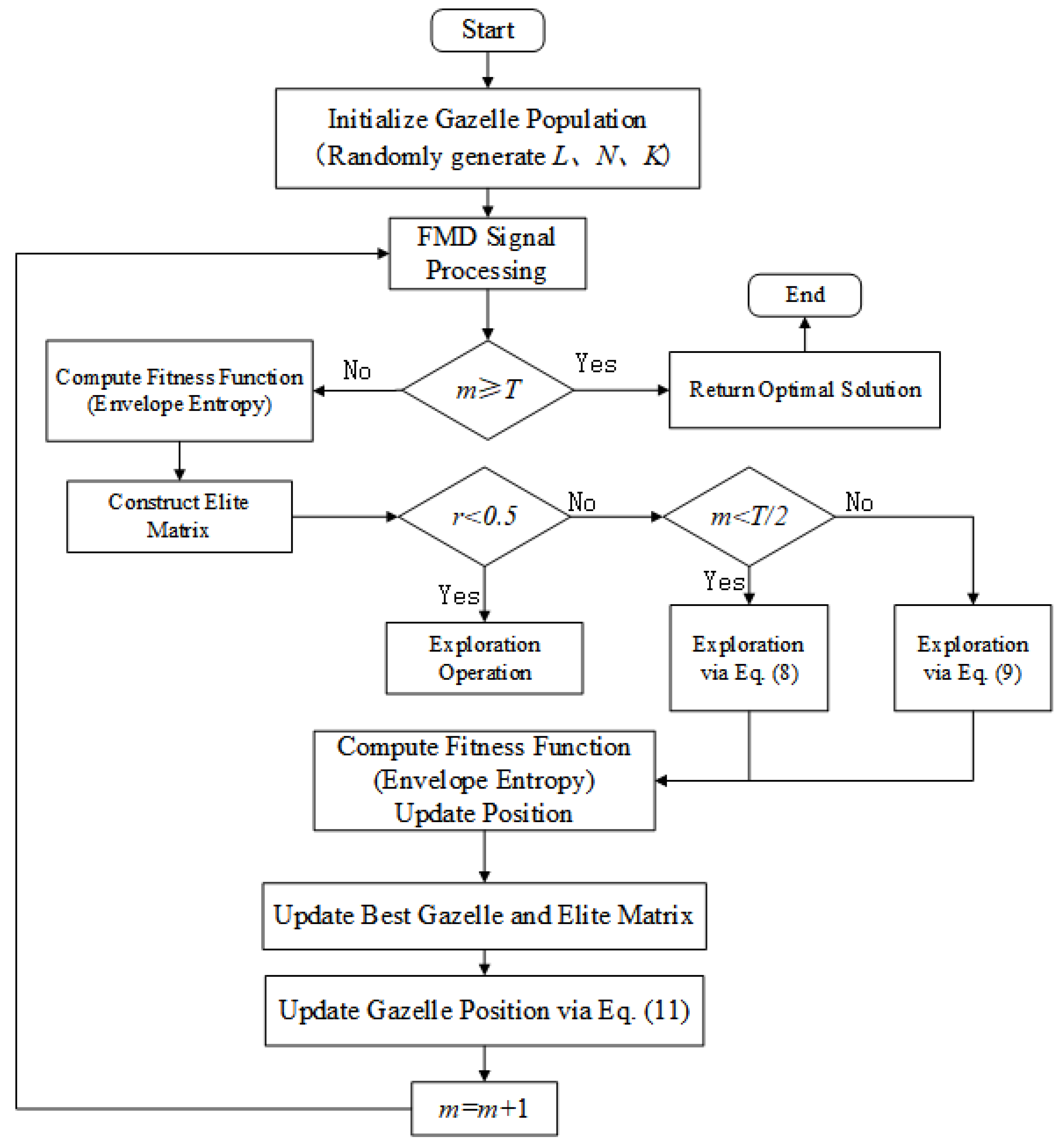
This work utilizes the GOA to optimize three parameters of the FMD process: the number of filters K, the filter length L, and the mode number N. The algorithmic flow for GOA-based parameter optimization is depicted in Figure 2. In the diagram, $r\in [0,1]$ denotes a uniformly distributed random number, and T represents the predefined maximum number of iterations, while m indicates the index of the current iteration.

Each gazelle represents a parameter combination {L, K, N} corresponding to the filter length, the number of filters, and the mode number, respectively. FMD is applied to the original signal using these parameters, and the envelope entropy of the decomposed signal is used as the fitness function, which is defined as follows:

$$E{n}_k=-\sum _{k=1}^N{p}_{k}lg\left(p_k\right)$$

(13)

$$p_k=a_k/\sum _{k=1}^N{a}_k$$

(14)

In these equations, a_k corresponds to the amplitude value of the k-th component in IMF set after envelope extraction, and p_k is the normalized amplitude. A lower envelope entropy implies that the extracted features are more concentrated and that the noise is reduced, which is advantageous for accurate fault identification [30,31].

2.3. Time Domain Feature Extraction from Vibration Signals

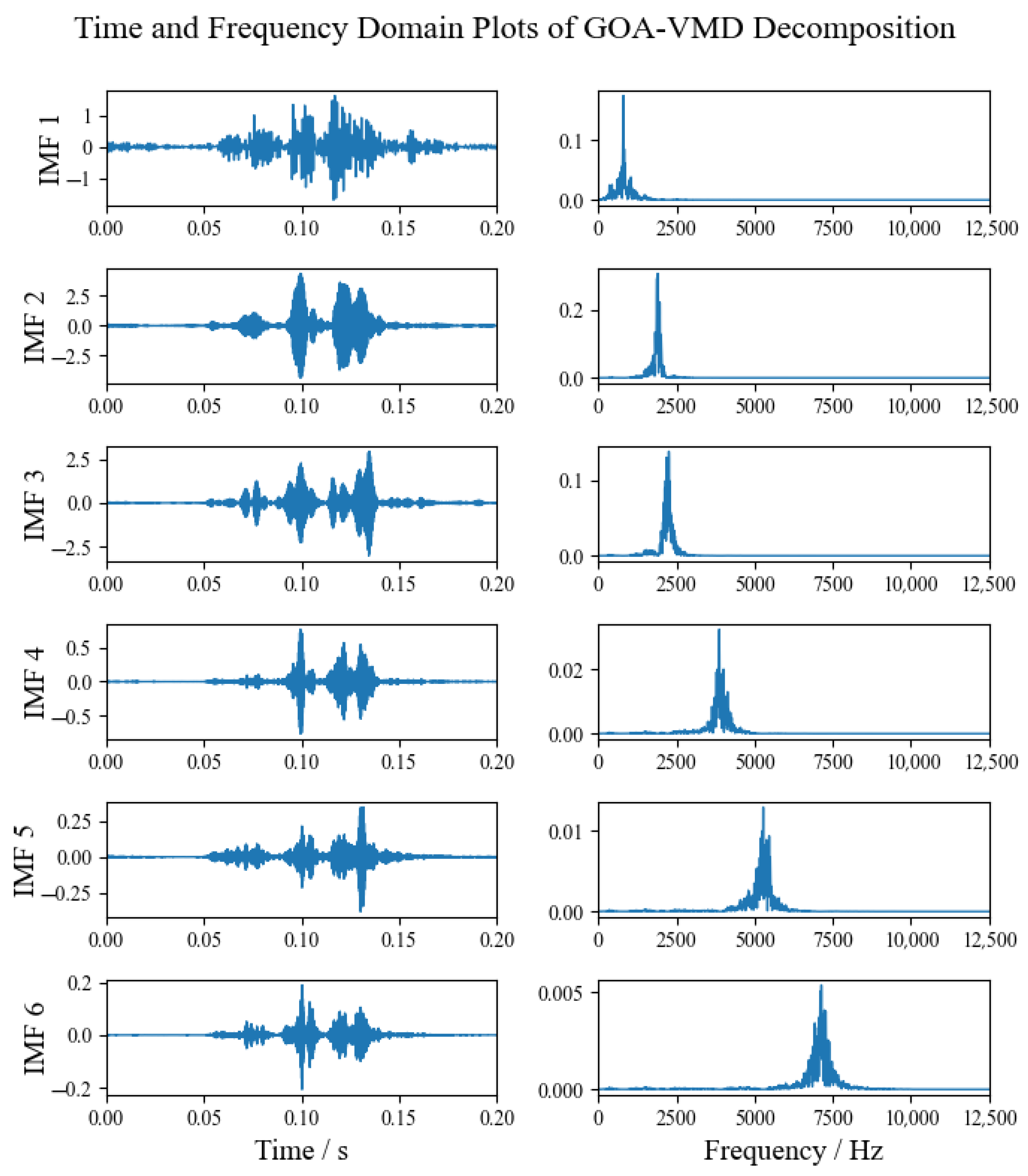
The FMD process generates IMFs, each corresponding to specific frequency bands of the OLTC vibration signals, thereby capturing critical information reflective of the system’s operational state. In order to characterize the impulsive and oscillatory behavior of the signal, four typical statistical indices in the time domain—namely peak factor, impulse factor, waveform factor, and margin factor—are computed from the IMFs [32,33,34,35].

The peak factor (PF), which quantifies the signal’s sharpness or impulsiveness, is mathematically described as follows:

$$PF={\displaystyle \frac{\max (|x(n)|)}{\sqrt{\frac{1}{N}{\displaystyle \sum _{n=1}^N}{x}^2(n)}}}$$

(15)

A high peak factor typically reveals sudden transient phenomena within OLTC vibration signals, often caused by mechanical shocks or abrupt contacts. The impulse factor (IF) reflects the impulsiveness of the signal and is expressed as follows:

$$IF={\displaystyle \frac{\max (|x(n)|)}{\frac{1}{N}{\displaystyle \sum _{n=1}^N}|x(n)|}}$$

(16)

For impact-type faults in OLTC systems, the impulse factor tends to exhibit significantly elevated values. The waveform factor (WF) describes the waveform characteristics and distortion level of the signal. It is computed by the following:

$$WF={\displaystyle \frac{\sqrt{\frac{1}{N}{\displaystyle \sum _{n=1}^N}{x}^2(n)}}{\frac{1}{N}{\displaystyle \sum _{n=1}^N}|x(n)|}}$$

(17)

This metric is frequently employed to assess the extent of waveform deformation and to distinguish periodic shock patterns from stochastic noise elements in the signal. The margin factor (MF) reflects whether the signal contains isolated high peaks, and is defined as follows:

$$MF={\displaystyle \frac{\max (|x(n)|)}{{\left(\frac{1}{N}{\displaystyle \sum _{n=1}^N}{x}^4(n)\right)}^{1/4}}}$$

(18)

This indicator evaluates whether the signal is approaching an extreme operating condition. A relatively large margin factor implies the presence of a prominent, isolated peak in the signal, which often corresponds to a transient event or an abnormal operating state.

2.4. Transformer-Based Classification Model Architecture and Implementation

The multiple intrinsic mode functions (IMFs) derived from the decomposition of the OLTC vibration signals exhibit varying levels of significance and distinct time domain characteristics. In addition, potential correlations may exist among the IMFs, which necessitate that classification models account for inter-feature dependencies. The Transformer, recognized as a cutting-edge deep learning framework, excels in modeling sequences and capturing global feature relationships, rendering it highly effective for handling intricate temporal data [21,22,36].

The proposed Transformer-based classification model comprises an encoder module and a classification head. The model receives a 24-dimensional input vector, derived by calculating four time domain statistical indicators from each of the six extracted IMFs. Positional encoding is initially added to preserve the sequential information. The encoded input is then processed by a multi-head self-attention mechanism, consisting of two encoder layers with four attention heads each and a model dimensionality of 128. The processed output is passed through a dense layer containing 64 neurons, followed by a Dropout operation set at a rate of 0.1 to reduce the risk of overfitting. Finally, a Softmax activation layer is employed to produce the classification probabilities. The schematic diagram of the designed model architecture is shown in Figure 3.

To ensure both robust feature representation and architectural simplicity, the model is tailored for fault diagnosis, particularly in cases with scarce annotated data [37]. The configuration parameters employed in the Transformer model are summarized in

Table 3. Hyperparameter settings of the Transformer model used for OLTC fault classification.

Parameter Name	Value/Type
Input Feature Dimension	24
Learning Rate	0.002
Number of Attention Heads	4
Total Attention Dimension	128
Optimizer	Adam
Number of Attention Layers	2
Feedforward Hidden Dimension	64
Output Category Dimension	4
Dropout Rate	0.1
Loss Function	Cross-Entropy
Classification Function	Softmax
Maximum Training Epochs	150

.

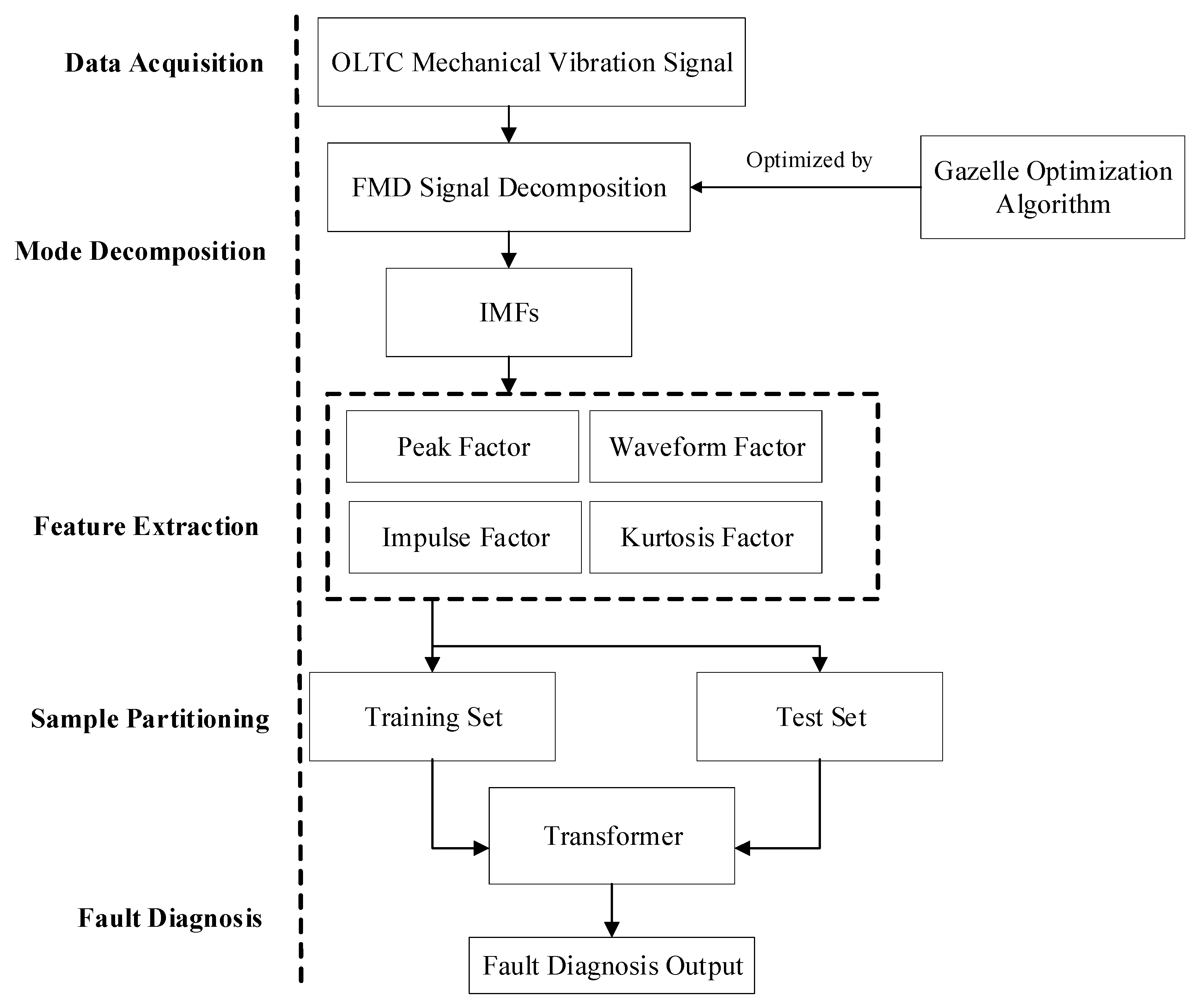
Based on the aforementioned model architecture and training configuration, the proposed OLTC mechanical fault diagnosis framework consists of five key stages: data acquisition, modal decomposition, feature extraction, sample construction, and fault classification. The overall process is illustrated in Figure 4.

3. Simulation of Mechanical Faults in OLTC

3.1. Experimental Platform Setup and Vibration Signal Acquisition

In this study, an experimental configuration for the KM-type OLTC was deployed to simulate vibration responses under both normal operating and representative mechanical fault conditions. A domestically manufactured KM-III800Y/126C-10193W OLTC prototype served as the test subject. Although the platform is based on a KM-type OLTC, the proposed method is not device-specific and is applicable to other OLTC models with similar mechanical structures. Vibration signals were acquired during the tap changing operation, providing empirical data to support the subsequent fault diagnosis research. The platform was instrumented with accelerometers (model YD38D, 100 mV/g sensitivity). The sensors were mounted in a triangular configuration on the top insulating cover of the OLTC unit, with their sensing axes oriented vertically (axial direction) as illustrated in Figure 5. This layout was chosen based on preliminary tests indicating that vibrations in the vertical (axial) direction consistently exhibited the highest amplitude in response to mechanical disturbances. In contrast, lateral directions were more susceptible to structural shaking and installation-related deviations during the tap changing operation, which could introduce measurement bias. Therefore, aligning the sensor axes vertically ensures measurement stability for vibration-based diagnostics. The triangular layout improves the spatial coverage and helps capture the localized vibration responses caused by different fault types.

The data acquisition system is capable of performing the multi-channel synchronous capture of vibration signals, offering a peak sampling frequency of 102.4 kHz. Considering that most of the energy in OLTC vibration signals lies below 10 kHz [38,39], a sampling frequency of 25 kHz was adopted in accordance with the Nyquist criterion to maintain signal fidelity and measurement accuracy [40].

3.2. Fault Type Setup and Analysis of Vibration Response Characteristics

To analyze the vibration characteristics of the OLTC under different fault conditions, three types of typical mechanical faults were introduced in the experiment (see Figure 6): (a) gear jamming in the drive shaft, (b) loose screw in the drive shaft, (c) arc plate looseness and contact wear. These fault types were selected based on their high occurrence frequency in engineering practice, ease of simulation on the experimental platform, and their capacity to generate distinguishable vibration features [6]. Specifically, gear jamming and screw looseness affect the torque transmission and stability of the drive mechanism, while arc plate and contact wear degrade electrical continuity and switching performance—both contributing to observable mechanical anomalies.

Under normal operating conditions, the structural components of the OLTC remain intact, and the contact mechanism functions without obstruction or abnormal friction. To simulate the gear jamming fault of the drive shaft, metal shims were inserted into the gear gaps to artificially introduce abnormal frictional torque between the gear teeth. The screw loosening fault was replicated by partially loosening the locking screw mounted on the drive shaft. The cam plate loosening fault was simulated by loosening its mounting screw, resulting in relative displacement between the cam and adjacent mechanical components. In addition, contact head wear was simulated under the same setup to reflect the degradation that typically co-occurs with cam plate looseness.

The vibration signal was recorded beginning at the instant the tap changer was actuated, with a total acquisition duration of 0.2 s and a sampling rate of 25 kHz, thereby capturing the complete switching process. To obtain a unified and noise-reduced signal representation, the raw signals from the three accelerometers were first synchronized and then averaged point-by-point across all sampling instances. This signal-level fusion approach helps suppress sensor-specific disturbances while preserving the global vibration characteristics, thereby enhancing the quality of the subsequent decomposition and feature extraction process. The corresponding waveform plots for this process are presented in Figure 7a–d, which clearly illustrate the variations in vibration response under different mechanical fault conditions.

Under standard working conditions, as depicted in Figure 7a, the vibration signal displays a smooth and low-amplitude waveform, suggesting that the system operates in a steady and well-balanced state. In contrast, Figure 7b illustrates that gear jamming in the drive shaft induces sharp transient spikes and significant amplitude fluctuations, indicative of high-frequency impulse components caused by mechanical impact. In Figure 7c, the loosening of the drive shaft screw results in an overall increase in vibration amplitude; however, the observed peaks are less pronounced than those in the gear jamming scenario. Figure 7d reveals that cam plate looseness combined with contact head wear leads to waveform irregularities, the presence of sharp peaks, and substantial amplitude variations, reflecting persistent fault characteristics throughout the switching process. The comparative waveform analysis indicates that both the amplitude and duration of vibration signals are considerably greater under fault conditions than in the normal state. To further quantify these distinctions,

Table 4. Comparison of temporal and spectral attributes of vibration signals.

Condition	Peak Value (m/s2)	RMS (m/s2)	Dominant Frequency Band (Hz)
Normal Condition	4.05	0.65	630 ~ 1760
Gear Jamming in Drive Shaft	7.58	1.10	1210 ~ 2265
Loose Screw in Drive Shaft	8.15	1.03	1235 ~ 2365
Arc Plate Looseness and Contact Wear	9.46	1.11	1225 ~ 2180

presents the peak value, root mean square (RMS), and dominant frequency band associated with each operating condition [41].

As observed from Table 4, all fault conditions exhibit significantly higher root mean square (RMS) and peak values compared with the normal operating condition. In addition, the dominant frequency band demonstrates an upward shift under fault scenarios. These results suggest that the evolution of mechanical faults leads to an increased vibration intensity and the presence of higher-frequency components, thereby highlighting the distinct dynamic distinctive features corresponding to various fault categories.

4. Experimental Data Analysis

4.1. GOA-FMD-Based Feature Extraction and Results Analysis

In this study, the maximum number of iterations for FMD was set to 10. The parameters of the GOA were configured as follows: the velocity factor s was set to 0.88, the predator success rate PSRs was 0.34, the initial population size was 20, and the total iteration count of iterations for GOA was set to 80. The parameter search range and step size for FMD are summarized in

Table 5. Parameter search space, step size, and optimal values for GOA-optimized FMD.

Parameter Name	Search Range	Step Size	Optimal Value
Mode Number N	[3, 10]	1	6
Filter Length L	[10, 100]	2	32
Number of Filters K	[5, 20]	1	12

, where the constraint $N\le K$ is satisfied to ensure decomposition feasibility.

During the GOA optimization process, the fitness function utilized in the optimization process was envelope entropy, which facilitated convergence towards the global optimum. The convergence behavior depicted in Figure 8 indicates that the fitness function undergoes a gradual decline with successive iterations, eventually approaching a steady value, indicating that the algorithm gradually approaches the optimal solution. This behavior confirms both the convergence and the effectiveness of the proposed optimization strategy.

The vibration signal was decomposed using FMD, and multiple IMFs were extracted. Taking the signal under normal operating conditions as an example, its time domain and frequency domain representations can be seen in Figure 9. It is evident that the frequency bands of the individual IMFs have been effectively separated, with clearly defined boundaries and no mode aliasing. These observations confirm that the decomposition achieved a satisfactory performance under the current parameter configuration.

To ensure both computational efficiency and diagnostic accuracy, only the first six IMFs were retained for feature extraction. As shown in Figure 10, the cumulative energy contribution rate of the first six IMFs exceeds 99%, which means that these components preserve almost all the meaningful vibration information while eliminating redundant or noise-dominated higher-order IMFs.

For each decomposed IMF, four representative time domain statistical indicators—peak factor, impulse factor, waveform factor, and margin factor—were calculated to characterize vibration features.

Table 6. Comparative analysis of statistical time domain indicators extracted from vibration signals under various OLTC operating conditions.

Parameter Name	PF	IF	WF	MF
Normal Condition	17.94359	52.11423	2.64016	155.10672
Gear Jamming in Drive Shaft	21.81183	68.66109	3.14788	180.01859
Loose Screw in Drive Shaft	23.72575	63.28335	2.66728	170.87625
Arc Plate Looseness and Contact Wear	23.95823	63.25377	2.90436	161.58832

presents the results using IMF3 as a representative case.

Under fault conditions, all four time domain indicators generally exhibit higher values compared with the normal operating condition. Notably, the peak factor values for the “Loose Screw in Drive Shaft” and “Arc Plate Looseness and Contact Wear” cases both exceed 23, indicating the presence of strong impact components in the vibration signal. The margin factor also shows a significant increase, reflecting greater deviation from steady-state operation and a higher likelihood of transient disturbances. These four time domain features, extracted from each of the six IMFs—resulting in a 24-dimensional feature vector—are subsequently used as input for the Transformer-based fault classification model.

4.2. Fault Classification Model Construction and Performance Comparison

In this study, vibration signals associated with OLTC contact operation were collected under four distinct conditions: (1) normal operation, (2) fault 1, gear jamming in the drive shaft, (3) fault 2, loose screw in the drive shaft, (4) fault 3, arc plate looseness and contact wear. For each condition, 150 signal samples were acquired, leading to a cumulative total of 600 samples. Among them, 120 samples per class were assigned to the training dataset, while the remaining 30 were used for testing, resulting in 480 training instances and 120 testing instances overall.

4.2.1. Comparison of Feature Extraction Performance Across Signal Decomposition Methods

To validate the effectiveness of FMD, a comparative analysis was conducted using three benchmark signal decomposition methods: Empirical Mode Decomposition (EMD), Ensemble Empirical Mode Decomposition (EEMD), and Variational Mode Decomposition (VMD). To ensure a fair comparison, the GOA parameters were held constant across all methods. GOA was employed to optimize the key parameters of each decomposition technique, and the optimized parameter configurations are summarized in

Table 7. Parameter names, search ranges, and GOA-optimized values for each decomposition method (VMD, EMD, and EEMD).

Decomposition Method	Parameter Name	Search Range	Optimal Value
VMD	Number of Modes	[2, 10]	6
	Penalty Factor	[100, 5000]	2621
EMD	Stopping Criterion	[1 × 10−6, 1 × 10−2]	1 × 10−4
	Maximum Number of IMFs Allowed	[3, 10]	6
EEMD	Noise Amplitude	[0.1, 0.5]	0.2
	Number of Ensemble Trials (Additive Noise)	[50, 500]	200

. The baseline decomposition methods, including EMD, EEMD, and VMD, were re-implemented by the authors based on the algorithmic descriptions and parameter settings reported in the relevant literature [9,11,42].

The OLTC vibration signals were decomposed using different signal decomposition methods (FMD, VMD, EMD, and EEMD). For each method, the same set of time domain features was extracted and used as the input to an identical Transformer-based classification model. To evaluate the fault identification performance of each decomposition technique, classification accuracy and confusion matrices were analyzed under consistent model configurations. The comparative classification results are presented in Figure 11 and summarized numerically in

Table 8. Classification accuracy of OLTC fault diagnosis using different GOA-optimized signal decomposition methods with Transformer-based classification.

Decomposition Method	Normal	Fault 1	Fault 2	Fault 3	Overall
GOA-FMD	100%	90.00%	93.33%	100%	95.83%
GOA-VMD	93.33%	76.67%	80.00%	96.67%	86.67%
GOA-EMD	80.00%	73.33%	70.00%	73.33%	74.17%
GOA-EEMD	90.00%	70.00%	80.00%	80.00%	80.00%

.

Among the tested decomposition methods, the GOA-FMD achieved the highest classification performance, with an overall accuracy of 95.83%. Notably, it reached near-perfect accuracy under both the normal operating condition and fault 3 (arc plate looseness and contact wear). In comparison, the GOA-VMD approach attained an overall accuracy of 86.67%, but exhibited noticeable performance degradation in identifying fault 1 (gear jamming). The GOA-EMD and GOA-EEMD methods yielded lower overall accuracies of 74.17% and 80.00%, respectively. These results suggest that GOA-FMD offers superior classification accuracy and robustness for OLTC vibration signal analysis, making it more suitable for practical fault identification applications. A five-fold cross-validation was performed for all methods to ensure a consistent and unbiased performance evaluation, as shown in Figure 12.

As shown in Figure 12, the GOA-FMD method achieved the best performance under five-fold cross-validation, with an average classification accuracy of 96.7%. This result highlights its effectiveness in suppressing mode mixing and enhancing both feature extraction and fault recognition accuracy. The GOA-VMD method attained an average accuracy of 87.3%, outperforming both GOA-EMD (73.5%) and GOA-EEMD (79.7%). However, it still exhibited noticeable fluctuations across folds, indicating limited adaptability to varying signal characteristics. In contrast, the EMD-based methods suffered from considerable drops in accuracy in certain folds, suggesting a relatively weaker capability in handling signal interference and preserving fault-relevant features. In summary, the GOA-FMD framework demonstrates a superior classification performance, enhanced stability, and strong generalization ability, rendering it particularly effective for diagnosing OLTC faults when only limited data is available.

4.2.2. Performance Comparison of Classification Models in Fault Identification

To gain deeper insight into the effectiveness of the Transformer model for diagnosing OLTC faults, this study conducted comparative experiments with several classic classification models, including SVM, RF, and MLP. The goal of the comparison was to assess the classification accuracy and robustness of each model when trained and tested with the same feature inputs and experimental settings. These baseline models were reproduced by the authors based on established methods reported in prior studies [18,20,43]. The hyperparameter settings for all baseline models are detailed in

Table 9. Hyperparameter configurations of comparative classification models (SVM, RF, and MLP).

Classification Model	Parameter Name	Value/Type
SVM	Penalty Coefficient	0.0009
	Kernel Function	Linear Kernel
RF	Minimum Samples Split	5
	Number of Trees	100
	Maximum Depth	10
MLP	Hidden Layer Size	(128, 64)
	Activation Function	ReLU
	Learning Rate	0.001
	Optimizer	Adam

. The hyperparameter settings for each baseline model were selected based on commonly accepted practices in the literature and fine-tuned through preliminary experiments to ensure optimal performance.

For consistency and a fair comparison, all classification models were trained using the same input features—namely, the 24-dimensional time domain feature vectors (comprising four statistical indicators extracted from six IMFs) obtained via GOA-FMD signal decomposition. The corresponding classification performance of each model is summarized in

Table 10. Classification accuracy of different models on the test set using GOA-FMD features.

Classification Model	Normal	Fault 1	Fault 2	Fault 3	Overall
Transformer	100%	90.00%	93.33%	100%	95.83%
MLP	90.00%	90.00%	80.00%	90.00%	87.50%
RF	86.67%	76.67%	76.67%	83.33%	80.83%
SVM	96.67%	76.67%	80.00%	80.00%	83.33%

and visualized in Figure 13.

According to the data in Table 10, the Transformer model demonstrated the greatest performance in OLTC fault classification, achieving an overall accuracy of 95.83%. It reached 100% accuracy in identifying both the normal condition and fault 3 (arc plate looseness and contact wear). In comparison, the MLP model attained an overall accuracy of 87.5%, but its accuracy for fault 2 (loose screw in drive shaft) dropped to 80.00%. The Random Forest (RF) model yielded an overall accuracy of 80.83%, with relatively poor classification results for fault 1 and fault 2 (both at 76.67%). The Support Vector Machine (SVM) model achieved 83.33% accuracy, indicating a more stable but consistently lower performance than the Transformer model. These results suggest that the Transformer model exhibits superior capability in capturing global and discriminative features from complex vibration signals. Its enhanced representation power makes it more suitable for high-precision fault classification tasks, particularly in the context of OLTC diagnostics.

As shown in Figure 14, the Transformer model obtained the greatest average classification accuracy of 96.8% across all five cross-validation folds, significantly outperforming the other benchmark models. This result highlights its strong ability to capture both the temporal dynamics and global representations inherent in OLTC vibration signals, thereby enhancing diagnostic precision. In contrast, the MLP model achieved an average accuracy of 89.5%, while the Random Forest (RF) and Support Vector Machine (SVM) models obtained 81.1% and 86.6%, respectively. All three models fell short of the Transformer’s performance in terms of both accuracy and stability. Such findings provide confirmation of the superior representational capacity and generalization ability of the Transformer model, confirming its effectiveness as a high-precision diagnostic framework for complex OLTC fault classification tasks.

5. Conclusions

This study investigates the mechanical fault diagnosis problem of the KM-type OLTC and proposes a novel classification framework that integrates GOA-FMD with a Transformer-based deep learning model. By incorporating vibration signal analysis, robust feature extraction, and advanced classification techniques, the proposed approach aims to enhance diagnostic accuracy and equipment reliability. The core conclusions drawn from the study are listed below:

1. A comprehensive experimental setup was established to simulate both normal and faulty OLTC operating conditions. Three representative mechanical fault types were introduced: fault 1—gear jamming in the drive shaft; fault 2—loose screw in the drive shaft; and fault 3—arc plate looseness and contact wear. A total of 600 vibration signal samples were acquired, providing a reliable data foundation for subsequent signal characterization and model training.

2. The vibration signals were decomposed using the GOA-optimized FMD method, in which key parameters—including the number of filters K, filter length L, and the mode number N—were adaptively optimized. This approach effectively suppressed mode aliasing and improved the separability of signal components. Subsequently, four time domain features (peak factor, impulse factor, waveform factor, and margin factor) were extracted from each IMF to construct a discriminative feature vector.

3. Comparative experiments among multiple decomposition methods (GOA-VMD, GOA-EMD, and GOA-EEMD) demonstrated that GOA-FMD achieved the best signal decomposition and classification performance. It obtained the highest average classification accuracy of 96.7%, significantly outperforming GOA-VMD (87.3%), GOA-EMD (73.5%), and GOA-EEMD (79.7%). These results confirm the superior fault feature preservation and anti-noise capability of GOA-FMD.

4. To perform fault classification, a Transformer model was adopted, which takes advantage of attention-based processing to extract global and long-range features from the input data. A comparative evaluation with classic models (SVM, RF, and MLP) revealed that Transformer achieved the best diagnostic performance on both the test set (95.83%) and in the five-fold cross-validation (96.8%), demonstrating a superior generalization ability and robustness under varying data conditions.

In conclusion, the proposed GOA-FMD + Transformer framework provides a feasible and scalable solution for intelligent condition monitoring and fault diagnosis in complex power equipment. The core innovation of this study lies in employing the GOA to adaptively optimize the key parameters of FMD, thereby achieving a superior signal decomposition performance. In addition, a Transformer-based classifier is introduced to enhance fault identification by leveraging its capability to model long-range dependencies in vibration signals. The integrated approach offers both a high diagnostic accuracy and practical engineering applicability. However, this study is limited to three predefined mechanical fault types. Further research is required to extend the approach to more diverse and complex fault scenarios to enhance its generalizability and deployment in broader real-world settings.