Optimizing Residential Electricity Demand with Bipartite Models for Enhanced Demand Response

Abstract

This study presents an advanced energy demand management approach within residential microgrids using bipartite models for optimal demand response. The methodology relies on linear programming, specifically the Simplex algorithm, to optimize power distribution while minimizing costs. The model aims to reduce residential energy consumption by flattening the demand curve through demand response programs. Additionally, the Internet of Things (IoT) is integrated as a communication channel to ensure efficient energy management without compromising user comfort. The research evaluates energy resource allocation using bipartite graphs, modeling the generation of energy from renewable and conventional high-efficiency sources. Various case studies analyze scenarios with and without market constraints, assessing the impact of demand response at different levels (5%, 10%, 15%, and 20%). Results demonstrate a significant reduction in reliance on external grids, with optimized energy distribution leading to potential cost savings for consumers. The findings suggest that intelligent demand response strategies can enhance microgrid efficiency, supporting sustainability and reducing carbon footprints.

1. Introduction

The increasing electricity demand, driven by the electrification of the residential, industrial, and transportation sectors, has intensified the need for more sustainable energy solutions. In parallel, the rise of renewable energy sources has introduced new dynamics of variability and uncertainty into power systems, requiring innovative strategies for management and operation. Distributed generation (DG) and demand response (DR) have emerged as key pillars of the energy transition, enabling deeper penetration of clean energy sources and optimized use of available resources [1,2].

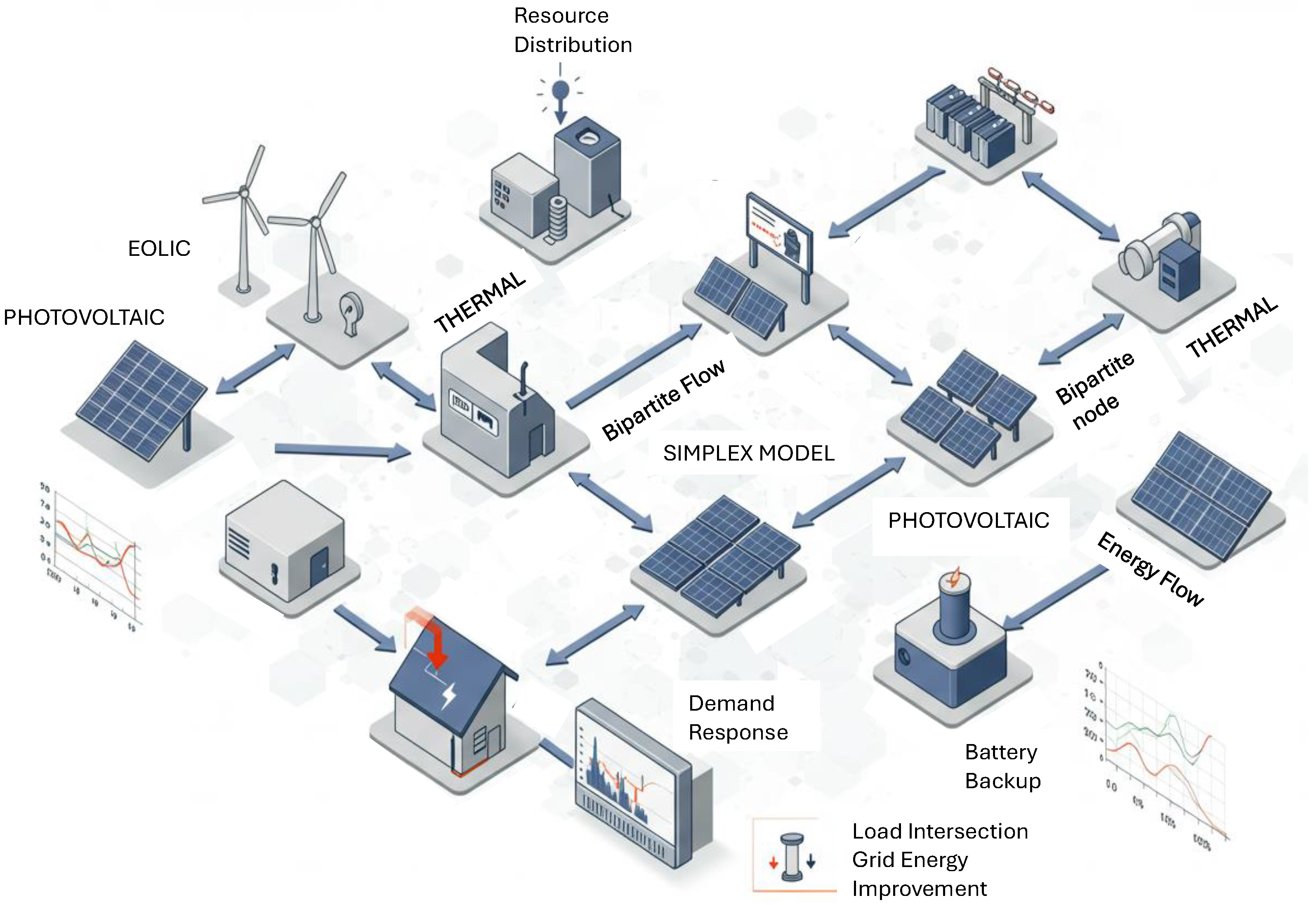
Nevertheless, a critical challenge persists: the optimal management of energy resources within microgrids that integrate multiple renewable sources, storage systems, and intelligent loads. Various studies have tackled this problem from cooperative and market-based perspectives (Figure 1). For instance, in [3], the authors propose an asymmetric Nash bargaining approach for cooperative operation among energy agents in systems integrating wind and hydrogen, demonstrating performance benefits in multi-agent scenarios but failing to explore structural allocation methods or the role of energy agent topologies. Similarly, in [1,2], the authors extend pole differential current-based protection schemes for bipolar LCC-HVDC lines, focusing on technical reliability without addressing optimization in local networks or residential demand management.

Within this context, the present study identifies a critical gap in the literature: the absence of structural models that explicitly capture the relationship between consumers and generators using bipartite mathematical frameworks.Such models can provide a powerful tool for representing, analyzing, and optimizing interactions in distributed energy systems. While existing literature prioritizes optimization algorithms and market strategies, no previous research has incorporated bipartite approaches to simultaneously manage energy allocation, demand response, and external grid independence—particularly in IoT-enhanced residential settings [4]. This study proposes an optimization model based on bipartite structures and the Simplex algorithm, applied to microgrids with smart devices. This approach provides an efficient graphical representation of the assignment problem between generation sources and consumer loads, promoting adaptive management that maximizes local generation, reduces losses, and limits dependency on the external grid [5,6]. In addition, the study explores a hybrid market scheme that combines spot transactions with long-term contracts, incorporating storage and DR as adjustment mechanisms [7,8]. This simplified market design stands in contrast to the complex cooperative models found in the literature [9], offering a feasible alternative for systems with lower technological or coordination maturity.

Implementation is contextualized in smart homes, where sensors and control platforms enable real-time decision-making regarding energy usage. The integration of bipartite modeling in this context introduces a novel analytical framework that combines network structures, optimization algorithms, and IoT technologies.

The bibliometric analysis (Figure 2) of literature published since 2020 reveals that, although there is growing interest in planning electricity consumption profiles in residential settings, none of the reviewed studies employed bipartite models. This finding underscores the originality of the proposed research: to provide an innovative framework combining mathematical, technological, and market-based tools for energy optimization in residential microgrids.

Background and Policy Context

Optimizing residential energy demand through intelligent microgrids plays a crucial role in achieving carbon neutrality targets around the world. This research aligns with the strategic goals outlined in major policy frameworks, such as the European Green Deal [10], which emphasizes digitalized, decentralized energy systems and a 55% reduction in greenhouse gas emissions by 2030. Similarly, the Sustainable Development Goal 7 (SDG7) of the United Nations promotes access to affordable and clean energy through renewable infrastructure [11], of which microgrids are a key enabler in low- and middle-income contexts.

At a technical level, international standards such as IEEE 1547 [12] and IEC 61850 [13] facilitate the interoperability of distributed energy resources and communication protocols in smart microgrid environments. In addition, empirical studies demonstrate that residential microgrids equipped with demand response and local storage can achieve CO₂ emission reductions between 25% and 45% compared to centralized configurations [14,15]. This study builds on these developments by proposing a reproducible and computationally efficient model that supports the global net-zero carbon transition.

This research sets itself apart from previous contributions by proposing an integrated framework that leverages three core technical innovations: (1) the formalization of the energy allocation problem using bipartite graphs, which model the dynamic relationships between distributed generation units and residential consumer loads; (2) the deployment of real-time IoT-based communication infrastructure, utilizing lightweight publish/subscribe protocols such as MQTT to enable decentralized demand response management; and (3) the hybrid integration of network topology modeling with linear optimization techniques (Simplex), offering a scalable and analytically tractable method for resource coordination.

Although recent studies have addressed robust optimization under uncertainty [5], agent-based control mechanisms [16], and heuristic or learning-based approaches for smart grids [3,6], none have proposed a unified architecture that simultaneously captures structural interdependencies via bipartite networks and solves the energy distribution problem using classical linear programming. In particular, the existing literature often focuses on algorithmic performance without an explicit representation of connectivity constraints between heterogeneous energy nodes and end-user loads. The methodology introduced herein not only fills this gap but also demonstrates practical feasibility through a set of high-resolution simulations and scenario-based analyses. These include both market-influenced and market-agnostic operational regimes, allowing a comparative evaluation of demand response strategies under variable pricing, resource saturation, and load prioritization. This comprehensive evaluation aligns with current efforts in the literature that call for greater integration of communication technologies, optimization, and system-level modeling in the context of decentralized energy systems [17,18].

2. Methodology

The methodology used in this study is based on a mathematical and computational approach to optimizing demand-side management in residential microgrids. Bipartite models are implemented for resource allocation, using the Simplex algorithm as the primary tool for optimizing energy flows. The methods used in the research are detailed below.

2.1. Microgrid Modeling

Microgrids are autonomous electrical systems that integrate multiple sources of renewable generation, energy storage, and electrical loads. In this study, a microgrid with photovoltaic, wind, and battery storage sources is modeled considering the interaction with the external grid.

• Wind Energy Aerodynamic models are used to calculate the power output of wind turbines, considering factors such as wind speed and air density. Equations relating the power coefficient and the angular velocity of the blades are used [9,19].
• Photovoltaic Energy A model based on the current–voltage (I-V) curves of solar panels is used, considering variations in irradiance and temperature [1]. Battery Storage: Batteries are modeled using equations that describe their capacity, depth of discharge, and self-discharge. Slow and fast charging models are considered to evaluate their impact on the microgrid [16].

2.2. Resource Allocation Using Bipartite Graphs

The optimal allocation of resources in the microgrid is represented by a bipartite graph, where nodes correspond to generators and loads, and edges represent the energy connections between them [20].

2.3. Graph

A graph is defined as the representation of the elements of a set and the relationships between them, based on binary relationships. These consist of a point in space. Of course, these can be connected by a line, which are called an edge, and the points can be called vertices or nodes. It is worth noting that a graph only contains information about connectivity.

2.4. Bipartite Graph

If we start from a graph $G=(N,E)$, it is said that, if the set of nodes containing the graph can be divided into two non-joining and non-empty sets of nodes $N_1$ and $N_2$, as shown in Equation (1).

$$N_1\cup N_2=N\mathrm{y}{N}_1\cap N_2=⌀$$

(1)

Let a bipartite graph be defined as $G=(U,V,E)$, where the following holds:

• $U=\{g_1,g_2,\dots ,g_m\}$: Set of distributed energy generators.
• $V=\{c_1,c_2,\dots ,c_n\}$: Set of consumers (loads).
• $E\subseteq U\times V$: Set of feasible allocation links between generators and consumers.

• Decision Variables

• $x_{ij}$: Energy assigned from generator $g_i$ to consumer $c_j$ [kWh].
• ${\delta }_j$: Demand reduction ratio for consumer $c_j$ due to demand response (DR).

• Objective Function

Minimize the total cost of energy allocation and include incentives for load reduction:

$$\begin{array}{cc}\hfill \underset{x_{ij},{\delta }_j}{min}& \sum _{(i,j)\in E}{C}_{ij}·x_{ij}-\sum _{j=1}^n{\lambda }_j·{\delta }_j·D_j^{\mathrm{load}}\hfill \end{array}$$

(2)

where:

• $C_{ij}$: Cost per kWh from generator $g_i$ to consumer $c_j$.
• ${\lambda }_j$: Incentive per reduced kWh for consumer $c_j$.
• $D_j^{\mathrm{load}}$: Nominal demand of consumer $c_j$.

• Constraints

• Generator Capacity Constraint

  $$\begin{array}{cc}\hfill \sum _{j=1}^n{x}_{ij}& \le P_i^{\mathrm{gen}},\forall i=1,\dots ,m\hfill \end{array}$$

  (3)
• Adjusted Demand Satisfaction
  Consumer demand must be satisfied after applying demand response:

  $$\begin{array}{cc}\hfill \sum _{i=1}^m{x}_{ij}& \ge D_j^{\mathrm{load}}·(1-{\delta }_j),\forall j=1,\dots ,n\hfill \end{array}$$

  (4)
• Demand Reduction Limits

  $$\begin{array}{cc}\hfill 0\le {\delta }_j\le {\beta }_j,& \forall j=1,\dots ,n\hfill \end{array}$$

  (5)
• Non-negativity

$$\begin{array}{cc}\hfill x_{ij}\ge 0,& \forall (i,j)\in E\hfill \end{array}$$

(6)

$$\begin{array}{cc}\hfill {\delta }_j\ge 0,& \forall j=1,\dots ,n\hfill \end{array}$$

(7)

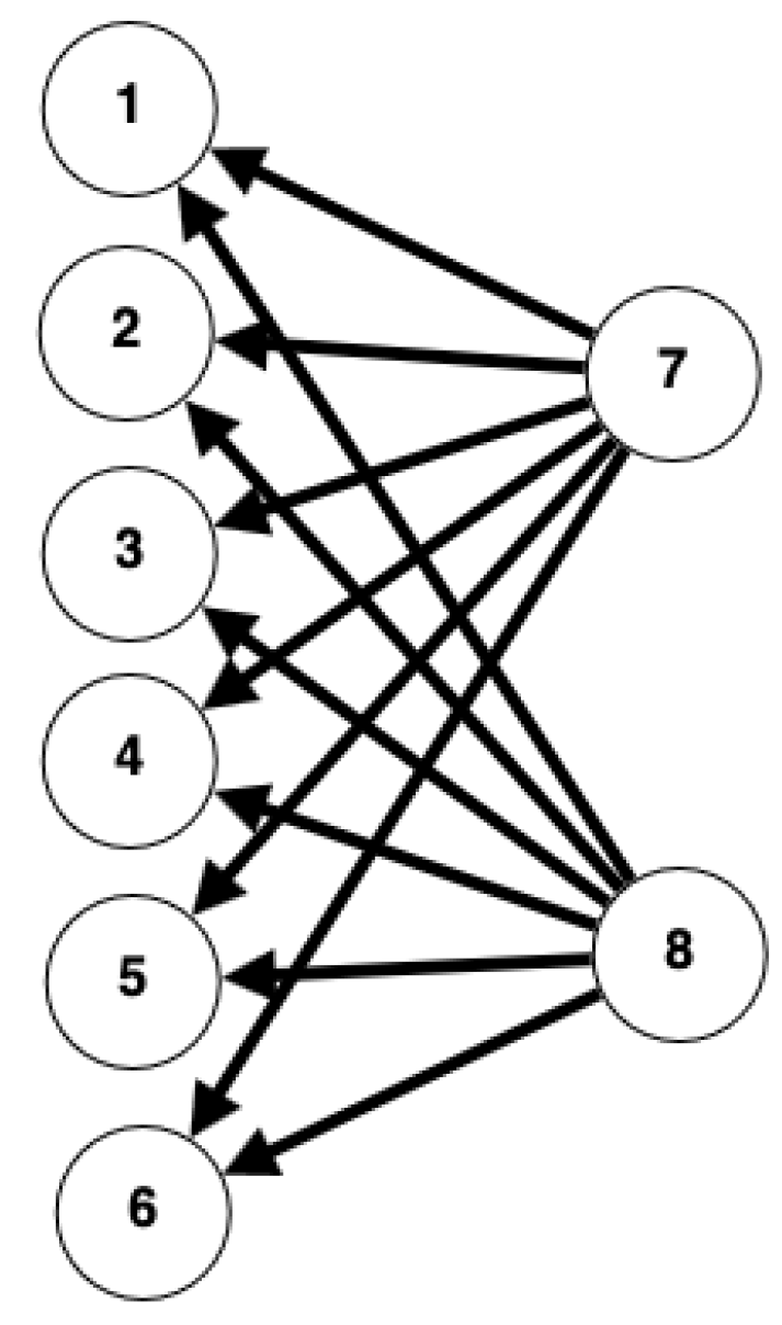
In short, each node in the set $N_1$ is adjacent to or connected to the nodes in the set $N_2$. Similarly, a complete bipartite graph is said to exist as long as there is adjacency or connectivity between all the nodes (Figure 3).

2.5. Optimization with the Simplex Algorithm

The Simplex algorithm is used to solve the energy allocation optimization problem, which is posed as a linear programming problem. Figure 4 presents a flowchart corresponding to Algorithm 1.

Algorithm 1 Optimal resource allocation

1: Start and initialize all modules  2: Input: Technical data from generators, Generators $U=\{g_1,g_2,...,g_m\}$, Consumers $V=\{c_1,c_2,...,c_n\}$  3: Input parameters: $C_{ij}$, $P_i^{\mathrm{gen}}$, $D_j^{\mathrm{load}}$, ${\lambda }_j$, ${\beta }_j$  4: Initialize variables: Dataset  5: Create bipartite graph $G=(U,V,E)$  6: Datase=data([GEN],[POT],[RD],[DEM])  7: define number of time intervals for the assignment:  8: for $i=1$ to 24 step $0.05$ do  9:     Generate empty graph 10:     Grafo=nx.Graph() 11:     Search for nodes in dataset to establish generation and demand 12:     Dataset[’s’]=Required generation 13:     Dataset[’l’]=Required Demand 14:     For each generator $g_i$ and each consumer $c_j$:     - Define edge $(g_i,c_j)$     - Assign cost $C_{ij}$ and capacity $x_{ij}^{max}$     - $x_{ij}\ge 0$: energy from $g_i$ to $c_j$     - ${\delta }_j\in [0,{\beta }_j]$: demand reduction at $c_j$ 15:     Minimize: ${\sum }_{(i,j)\in E}{C}_{ij}·x_{ij}-{\sum }_{j=1}^n{\lambda }_j·{\delta }_j·D_j^{\mathrm{load}}$ 16:     ${\sum }_{j=1}^n{x}_{ij}\le P_i^{\mathrm{gen}}$ for all i ${\sum }_{i=1}^m{x}_{ij}\ge D_j^{\mathrm{load}}(1-{\delta }_j)$ for all j $0\le {\delta }_j\le {\beta }_j$ 17:     Solve the linear program using Simplex or LP solver 18:     Store optimal values: $[x_{ij}^{*},{\delta }_j^{*}]\leftarrow$ Optimize(G, objective, constraints) 19: end for 20: Fill network with all remaining dataset information 21: for $i=1$ to $dataset$ step $0.05$ do 22:     add.edge(Gen1(i),Load1(i),Weight(i),Capacity(i)) 23: end for 24: Add links to complete the flow network 25: add.edge(Requerid-Generation,Generator) 26: add.edge(Generator,Requerid-Demand) 27: Execute Simplex network method: 28: FlowDict=nx.network simplex(Grafo) 29: Create an empty network storing the step response 17 30: GrafoN=nx.Graph(flowDict) 31: remove required generation and demand nodes 32: GrafoN=GrafoN.drop($Nod{e}_s,Nod{e}_l$) 33: generation of results in a network 34: Results graph 35: End

2.6. Reproducibility and Implementation Details

To ensure the reproducibility of this study, all simulations were developed using Python 3.9 with the NetworkX library (v2.8.4) for graph modeling, coupled with SciPy’s linear programming solver for Simplex optimization. The time-series data for load and generation profiles were sourced from public datasets and simulated with hourly resolution across a 24 h horizon, with a temporal granularity of 0.05 h per iteration.

The IoT integration is emulated using a virtual MQTT broker (Eclipse Mosquitto) for communication between demand-side devices and the central optimizer. Additionally, energy source parameters (efficiency, price, availability) are parameterized based on empirical references [21,22,23].

All scripts, data sources, and simulation setups have been organized in an open-access repository (link will be provided upon publication) to facilitate full methodological transparency.

Objective Function and Constraints

For this description, the example of maximizing generated power and minimizing losses in the microgrid will be used (Equation (8)).

$$max\sum _{(i,j)\in A}{C}_{i,j}{x}_{i,j}$$

(8)

where:

• $x_{i,j}\to$ Weight of each generator.
• $C_{i,j}\to$ Power of each generator.
• Constraints:
• Power balance: Generation must match demand.
• Transmission capacity: Each connection has a capacity limit.
• Generation costs: Energy costs are minimized by prioritizing renewable sources [5].

$$\sum _{(i,j)\in A}{x}_{i,j}-\sum _{(i,j)\in A}{x}_{j,i}=b\left(i\right)\forall i$$

(9)

$$l_{i,j}\le x_{i,j}\le u_{i,j}\forall (i,j)\in A$$

(10)

The method is implemented in an iterative process, ensuring that the solution is improved at each step until the optimal distribution of energy resources within the microgrid is achieved [24,25].

$$\overrightarrow{C_{i,j}}=C_{i,j}-\pi \left(i\right)-\pi \left(j\right)$$

(11)

$$\overrightarrow{C_{i,j}}=0\forall (i,j)\in B$$

(12)

$$\overrightarrow{C_{i,j}}\ge 0\forall (i,j)\in L$$

(13)

$$\overrightarrow{C_{i,j}}\le 0\forall (i,j)\in C$$

(14)

2.7. Demand Response

Demand response is a key strategy for reducing consumption during times of high demand and improving system efficiency.

Load ranking: An algorithm that classifies loads according to their priority and the possibility of being disconnected or shifted over time is implemented. Consumption reduction: Response levels of 5%, 10%, 15%, and 20% are applied to evaluate the impact on the demand curve. Impact assessment: An analysis is made of how demand redistribution affects the share of the external grid and the energy efficiency of the microgrid, as shown in Algorithm 2.

User engagement is a critical factor in the success of demand response strategies. In this model, participation is simulated algorithmically; however, practical deployment requires behavioral incentives and user-friendly interfaces. Studies have shown that combining dynamic pricing with feedback systems, such as mobile applications that visualize energy savings, can significantly improve user responsiveness [26]. Additionally, gamified demand reduction targets and financial rewards can increase sustained engagement, especially when coupled with IoT automation that minimizes manual user intervention.

Algorithm 2 Demand Response Algorithm

1: Start and initialize all modules  2: Input: Technical data from generators  3: Initialize variables: data, dat1, d1, d2  4: Generate ranking: Dataset ← data.rank(method="min")  5: Classify ranking into two groups:  6: if data.rank ≤ 10 then  7:     Dataset1 ← data  8: else  9:     Dataset2 ← data 10: end if 11: if Dataset1 > 10 then 12:     data.rank ← 0 13: else if Dataset1 ≤ 10 then 14:     data.rank ← 0 15: end if 16: Define percentage steps for demand response: 17: for $i=0.05$ to $0.20$ step $0.05$ do 18:     Estimate average: 19:     $s1\leftarrow \mathtt{sum}\left(d1\right[’Demand’\left]\right)$ 20:     $s1\leftarrow s1/\#\mathtt{of data points}$ 21:     if ranking data > 0 then 22:         $d1\leftarrow d1+s1$ 23:     else 24:         $d1\leftarrow 0$ 25:     end if 26: end for 27: Generate result dataset for Simplex algorithm: 28: Dataset.results← RD[’DEM’] 29: Generate result graph 30: End

2.8. Integration of the Internet of Things (IoT) in Energy Management

The Internet of Things (IoT) enables real-time communication between electrical devices and the microgrid management system.

Use of smart sensors: Sensors are used to monitor the energy consumption of residential devices. MQTT communication protocol: This protocol enables the connection between devices and the control platform [19]. Demand response automation: The system automatically adjusts device consumption in response to energy availability and changing electricity prices. The deployment architecture of the proposed microgrid management system follows a modular edge-cloud hybrid design. At the local (edge) level, smart meters and actuators communicate with a central controller using the MQTT protocol. This controller executes the optimization algorithm and manages load prioritization. Optionally, cloud-based dashboards collect usage statistics and optimization results to facilitate system monitoring and updates. This decentralized deployment enhances resilience and reduces latency in decision-making, aligning with best practices in modern distributed energy systems [26].

2.9. Comparative Perspective on Demand Management Strategies

In contrast to heuristic, rule-based, or agent-based demand management techniques, the bipartite graph-based optimization proposed in this work offers a mathematically rigorous and scalable framework. For example, heuristic approaches such as fuzzy logic controllers or neural networks excel in pattern learning but often lack transparency and convergence guarantees [27]. Agent-based strategies offer decentralized decision-making but may require extensive coordination overhead [28]. In our model, the Simplex algorithm ensures optimality under linear constraints, while the bipartite structure provides an explicit mapping between sources and loads, allowing for real-time and interpretable decision-making. This integration enables practical deployment in residential settings where system explainability, computational speed, and adaptability to IoT environments are paramount.

3. Study Problem

An exact method based on linear graph programming, known as the Simplex network solution method, is proposed to optimize resource allocation in generation and demand management, as illustrated in Figure 5 and Table 1. This approach maximizes the power delivered without waste while maintaining user comfort. Additionally, a ranking-based model is introduced as input for the load management algorithm, enabling devices or loads to be selected according to an optimal curve. The implementation is based on a broker where the Simplex algorithm manages the loads through MQTT communication, in line with the Internet of Things trend. For greater accuracy in modeling generation sources, georeferenced data for photovoltaic energy [23] and real datasets for wind energy [22] are utilized, while other sources employ equation-based models. The network solution is implemented with the NetworkX library [29].

To define the generation prices, we base ourselves on [21], so we have the following table.

Table 1. Parameters of the thermal generator park.

Generation Type	Price [cUSD/kWh]
Wind	9.13
Photovoltaic	40.03
Biogas	13.21
Geothermal	9.28
Hydroelectric	7.17

Table 1. Parameters of the thermal generator park.

Generation Type	Price [cUSD/kWh]
Wind	9.13
Photovoltaic	40.03
Biogas	13.21
Geothermal	9.28
Hydroelectric	7.17

An estimated load will be calculated, and, as mentioned, the resources available in the microgrid will be modeled on a given day. This is illustrated in Figure 6, which shows the availability of the grid under both conventional and non-conventional renewable energy sources, as well as the charging and discharging of the storage system.

Additionally, you can see the concentration of resources more clearly in Figure 7, along with Figure 6, which is a heat map, to see what type of resource has the most significant presence that day.

3.1. Case Study Analysis

The constant increase in greenhouse gases, industrial growth, the development of new technologies, and population growth—these sets of parameters will be reflected in the continuous expansion of residential electricity demand, which requires an ever-increasing increase in generation. However, the economic aspect will always be involved, which is why an analysis is proposed with and without an electricity market.

3.1.1. Analysis with an Electricity Market

This refers to predefining the weights and prices within the algorithm to find the most optimal generation from both economic and environmental perspectives, that is, generating at the lowest possible cost, taking into account the external grid.

3.1.2. Analysis Without an Electricity Market

When leaving the electricity market, the goal is to extract the maximum power flow from all generation sources in the microgrid. Therefore, the weights defined in the algorithm are small, forcing the model to allocate all resources within the microgrid to meet the single demand and attempt to exclude the external grid. In the event of surpluses in the microgrid, they can be evacuated to the grid.

3.1.3. Typical Daily Demand Curve

It is essential to note that the residential demand curve exhibits variations throughout the year; however, the model, when executed at each time interval, will adapt to the new condition each time. This means that weather disturbances will not affect demand. Therefore, an optimal demand response is proposed, based on demand behavior, to adjust demand through load management.

3.1.4. Analysis with Demand Response

It is necessary to utilize microgrid resources more effectively, thereby avoiding dependence on the external grid and recovering the investment made in a microgrid. Therefore, it is proposed to introduce the response to demand, which is varied in this analysis by 5%, 10%, 15%, and 20%.

4. Analysis of Results

Five analysis scenarios are carried out to evaluate the effectiveness of the proposed methodology:

To simulate a realistic residential environment, this methodology is conceptually applied to a suburban neighborhood based on the average characteristics of the “Valle de los Chillos” settlement near Quito, Ecuador, which consists of approximately 120 residential units per neighborhood. The typical daily load profiles used in the simulation reflect the aggregated consumption patterns of communities of similar size, allowing for the practical validation of demand response dynamics on a representative urban scale [31].

4.1. Scenario I

In Scenario I, the response to demand is implemented based on percentages. These are varied in 5% steps, starting from the typical demand, until a response to demand of 20%. Under these conditions, it can be seen that small peaks are generated during certain off-peak hours, of course, not at the level of the initial peak demand, because what is obtained is a redistribution of demand; as a ranking method used, this will project demand in a better way, thus saving resources for the end user’s network, without generating greater discomfort to the user. In this scenario, there is still no intervention with the different sources of generation or allocation of resources. The result is presented in Figure 8.

Based on the application of demand response, four additional scenarios are generated, which will examine how demand response influences resource allocation.

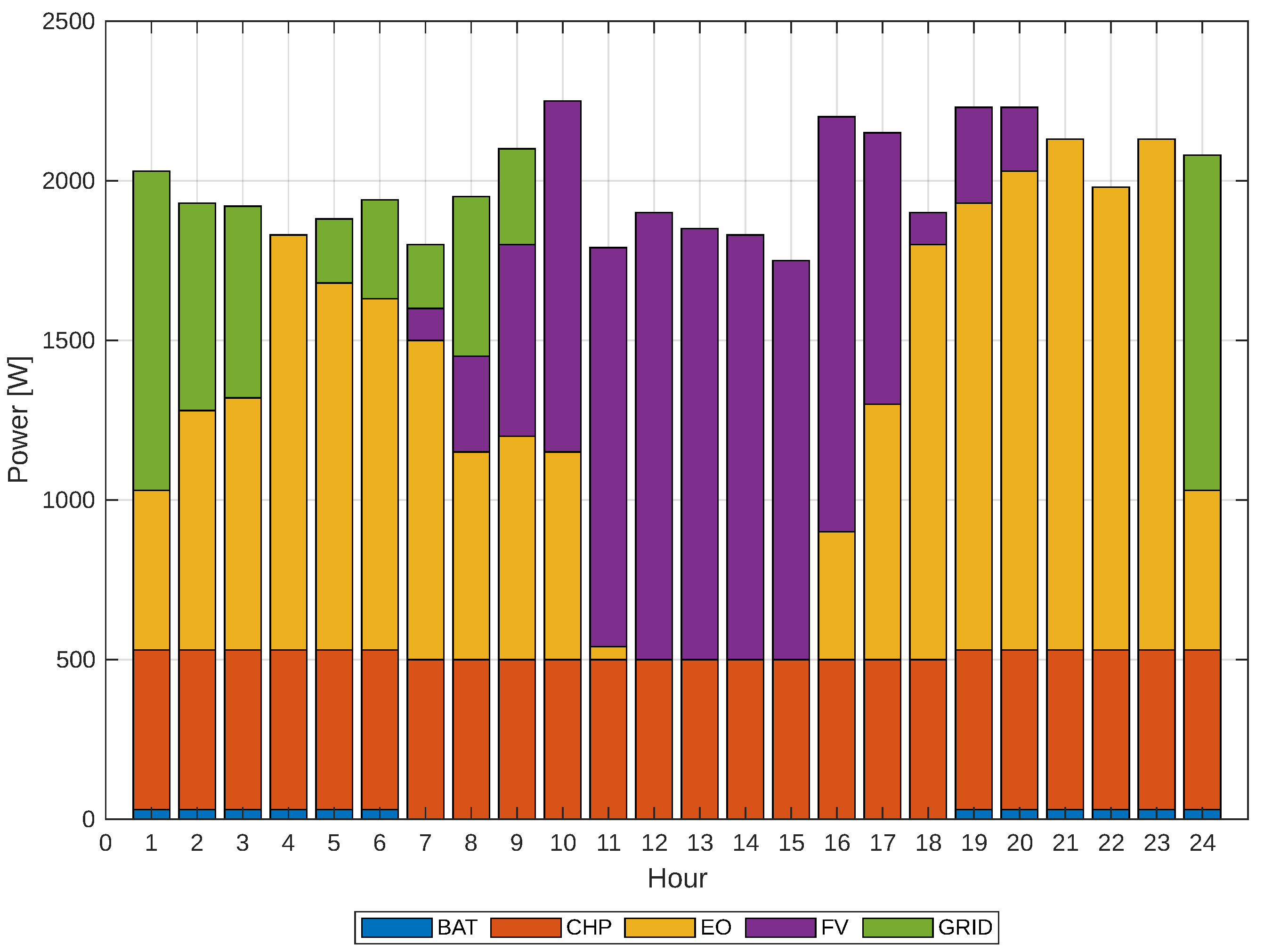
4.2. Scenario II

Scenario II will be generated based on a 5% demand response injection. In addition, based on this scenario, resource allocation will begin with the conventional and non-conventional power plants that comprise the microgrid, as well as storage systems. Their behavior is also taken into account when they are loaded and consumed from the microgrid, as well as when they are discharged and contribute to the microgrid. This is presented in the order of allocation, which is graphically represented in Figure 9. In general, a transition can be observed throughout the day with a greater presence of wind and photovoltaic energy. Furthermore, in this scenario, the algorithm allocates a smaller proportion of the external grid to supply the load, which is optimal in this context.

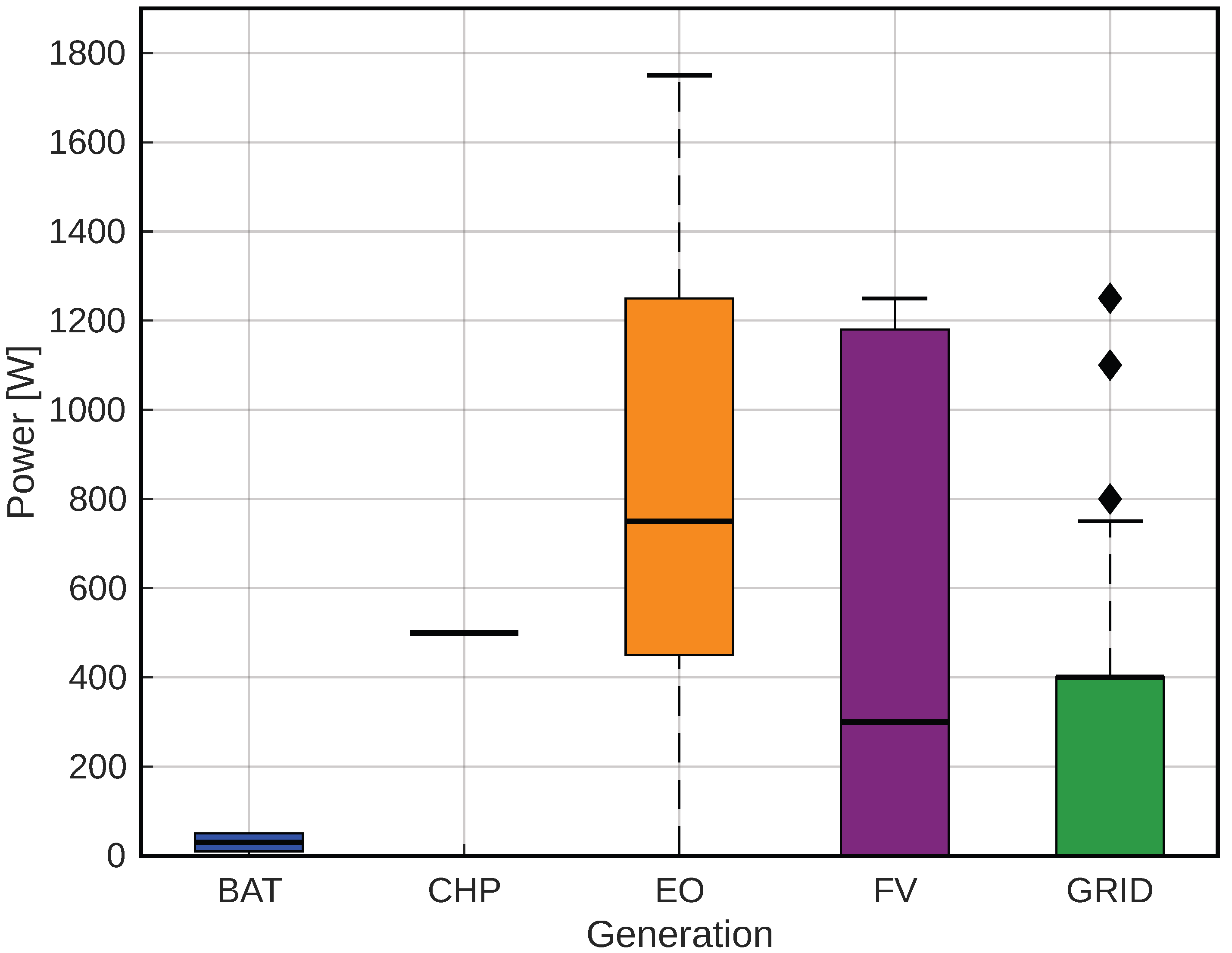
On the other hand, a more exhaustive analysis is carried out for each type of demand response, which involves generating box diagrams to observe the minimum and maximum contributions of each generation source and determine how much the external grid intervenes in each demand response.

It can be seen in Figure 10, which corresponds to a response to a demand of 5%, that there is still a considerable presence of the external grid supplying the loads, compared to the remaining generation sources; its presence is quite substantial.

4.3. Scenario III

In Scenario III, resource allocation is carried out in the same way, so the same amount of resources is used as in Scenario II, and an increasing demand response from 5% to 10% will be considered. The solution is presented graphically in Figure 11.

From this result, it follows that as demand response increases, the demand points in each interval begin to equalize, implying a flattening of the demand curve rather than exaggeration, which is necessary to adjust to reality. Furthermore, in interval 11, it is no longer possible to allocate wind energy in certain time intervals, since the demand response is greater, as seen in Figure 12.

Regarding the share of generation sources in the current scenario, the demand response is 10% (Figure 13). It can be observed that there is a slight decrease in the grid’s share compared to scenario II.

4.4. Scenario IV

A similar scenario is presented to the previous one, but the response to demand increases from 10% to 15%, as can be seen in the following graphical representation (Figure 13).

We can see that the demand points are no longer equal, so we can say that the flattening of the demand curve will tentatively occur at a 10% rate. Everything will depend on what is observed in Scenario V. In the current scenario, the share of generation sources in responding to demand is 15.

4.5. Scenario V

There is a scenario where a 20% response to the demand is injected, which will be determined in this case study as maximum and feasible; the solution is presented in Figure 14.

As in Scenario III, wind power is not assigned in four intervals (12, 13, 14, 15), and the same happens in the other scenarios, except the second scenario, which means that by increasing the response to demand, the load will be less dependent on generation, as well as on the external grid, so that surplus can be delivered instead of consumed in that time interval.

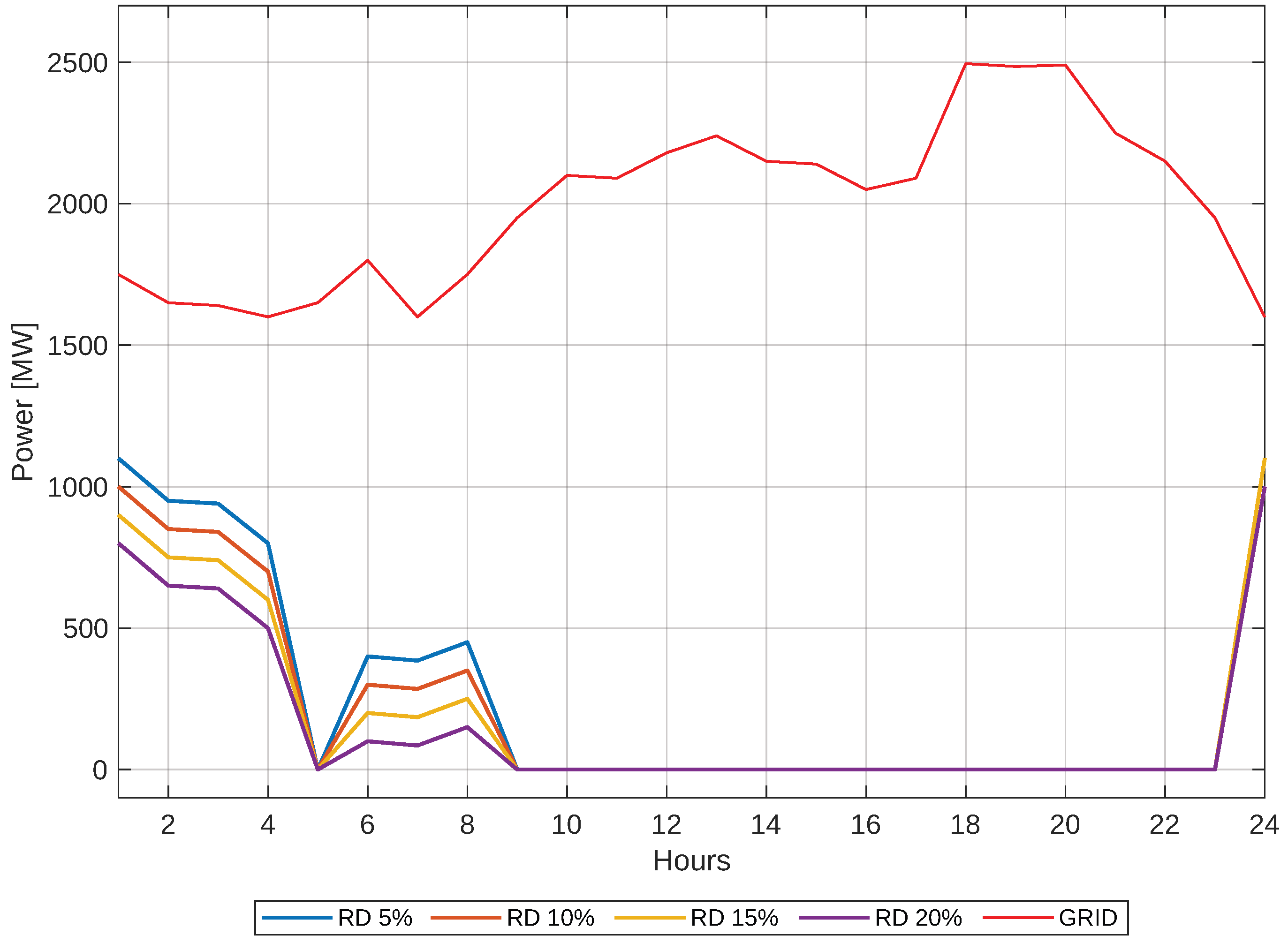
Finally, given the previous cases, it can be observed that the share of the grid decreases as the response to demand increases. The solution with a 20% demand response is shown in Figure 15. It is essential to understand how far our solution deviates from the typical demand curve, specifically whether we will be drawing power from the external grid or not, and whether the implemented model is optimal. Therefore, the comparison described above is presented in Figure 16.

4.6. Renewable Intermittency and Self-Sufficiency Considerations

Due to the inherent intermittency of renewable energy sources such as wind and solar, achieving consistent self-sufficiency at all hours of the day presents a significant challenge. In this study, the optimization model incorporates storage systems and dynamic load shifting to mitigate the intermittency of energy sources. Battery systems are modeled with variable charge/discharge cycles, which allows the system to store surplus energy during periods of excess generation and utilize it during demand peaks or low renewable output intervals. In addition, the demand response mechanism introduces flexibility by reshaping consumption patterns in real time, reducing stress on the system during declines in renewable generation. Although full 24 h autonomy is not guaranteed under all weather conditions, simulations show that with moderate storage capacity and a demand response level above 15%, the microgrid can reach near-complete self-sufficiency during 70–85% of the operating period. Future enhancements may include predictive models for generation forecasting to improve allocation efficiency and reliability of autonomy [5,32].

We can see that the solutions for the different demand response percentages and resource allocations are optimal, in some cases exceeding expectations, as when these curves approach zero, it means that there will be no consumption from the external grid. The point is reached where the energy produced can be contributed to the external grid and, in this way, recover the investment involved in a microgrid in less time. It’s essential to note that, despite demand response and management, there are periods when the grid is necessary, as energy sources are not constant.

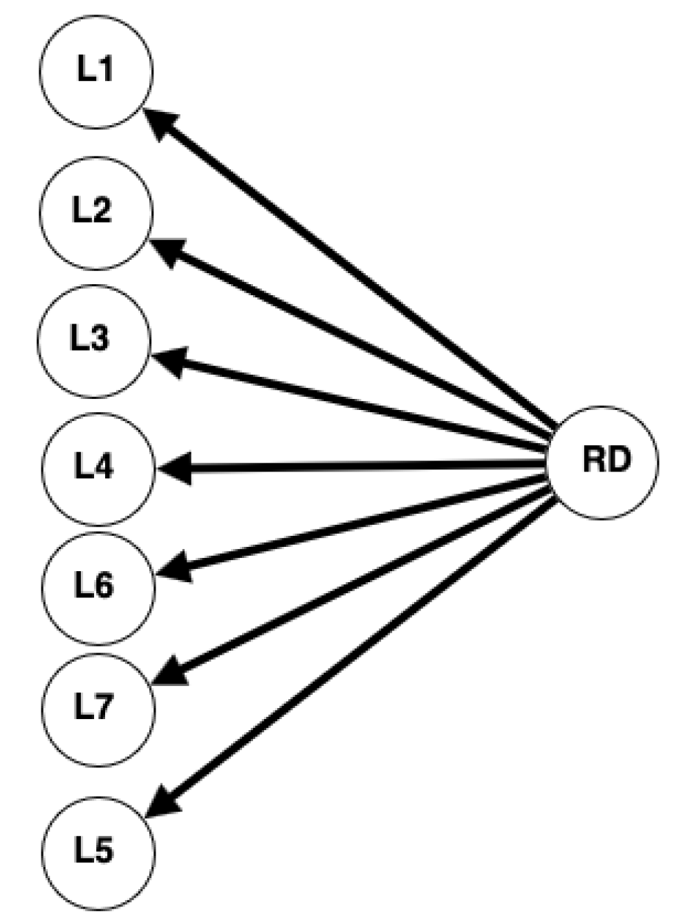
The energy that the user can save (Figure 15) is achieved by up to 100% over specific time intervals. On the other hand, we can observe the load management solution, represented by the graph (Figure 17), in a time interval. A scenario with several loads is proposed, and Simplex will assign the least important loads. L1, L2, L3, L4, L5, L6, and L7 are a set of loads, resulting in load L3 being unusable during that interval, unable to respond to the demand at that time.

4.7. Discussion

The results presented in this study confirm the effectiveness of bipartite graph models in improving the efficiency of demand response strategies within residential microgrids. As shown in Scenarios I–V, increased participation in responding to demand (from 5% to 20%) led to progressive reductions in dependence on the external grid, demonstrating a clear trend toward local energy autonomy. The optimal assignment of energy through the Simplex algorithm aligns with the findings of [5,24], which suggest that linear optimization frameworks are practical for managing energy demand. However, the novelty in this study lies in the integration of bipartite structures, which enable real-time energy allocation decisions, particularly when combined with IoT-based control systems, as supported by [19,23]. 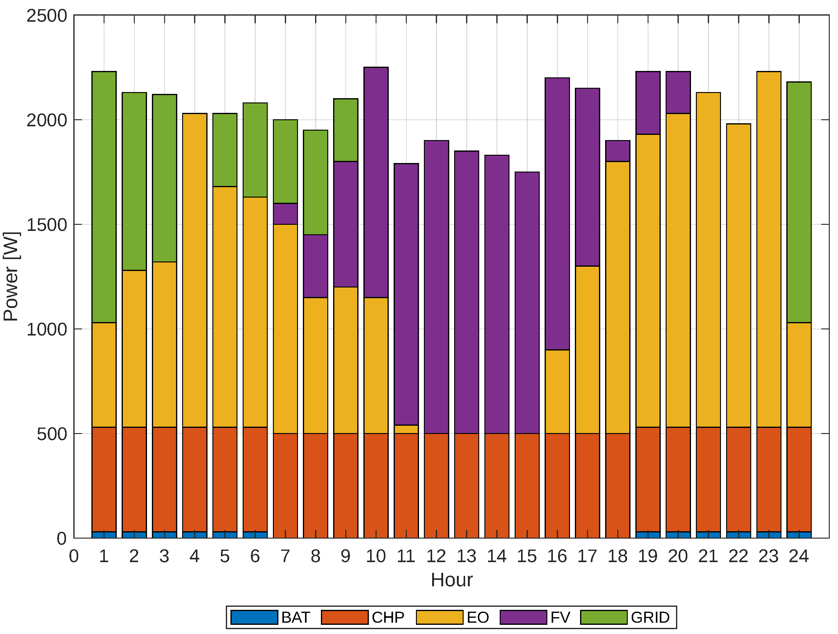Moreover, results suggest that grid independence peaks at around 20% demand response, validating theoretical claims in [25] about self-sufficiency through bi-level optimization. The implication is that microgrids with dynamic load flexibility can not only serve to reduce peak demand but also act as net contributors to the grid during surplus periods, as shown in Figure 18 and Figure 19. This approach bridges optimization and topology modeling, offering a dual benefit:

• a mathematically tractable allocation mechanism, and
• an intuitive network structure capable of supporting adaptive energy distribution in real-world applications.

Figure 18. Resource allocation based on demand response at 20%.

Figure 18. Resource allocation based on demand response at 20%.

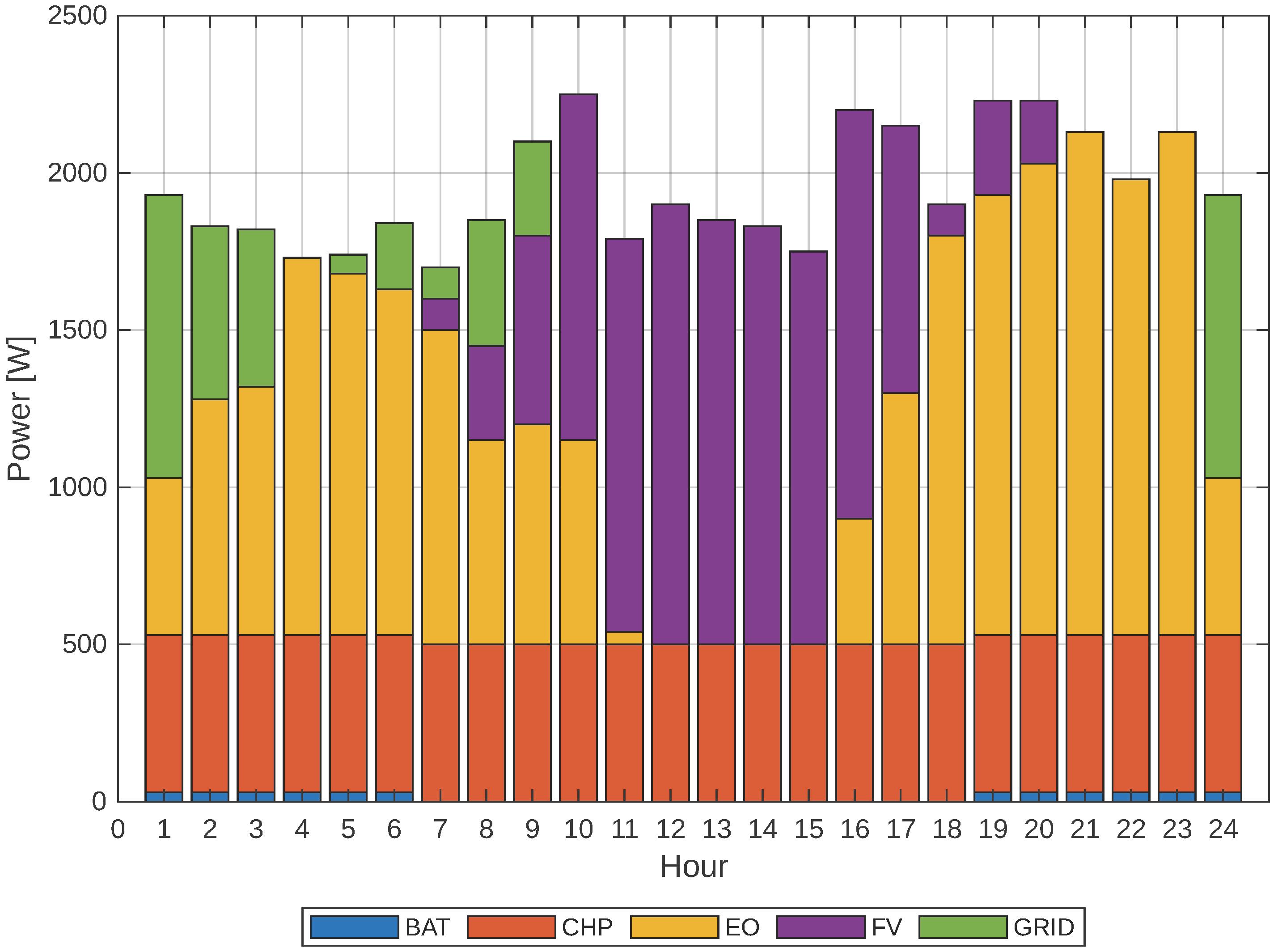
Figure 19. Presence of different types of generation, demand response at 20%.

Figure 19. Presence of different types of generation, demand response at 20%.

5. Conclusions

This study presents an optimized energy management strategy for residential microgrids using bipartite models and the Simplex algorithm to enhance demand response efficiency. The results demonstrate that implementing optimal resource allocation and demand response mechanisms can lead to significant improvements in energy consumption distribution and a reduction in reliance on non-renewable sources.

The proposed method effectively reduces dependency on the external grid, achieving up to 100% self-sufficiency in specific time intervals.

Demand response programs help flatten the load curve, redistributing consumption more efficiently and reducing peak loads.

The application of IoT-based energy management enables real-time control of electrical loads, optimizing energy use without compromising user comfort.

The Simplex-based optimization model ensures that power generation is maximized while minimizing losses and costs.

Limitations:

The variability of renewable energy sources affects the ability to maintain consistent self-sufficiency, necessitating the need for additional energy storage solutions.

The implementation of IoT infrastructure may require initial investments and technological adaptations.

The effectiveness of demand response depends on user participation and the availability of controllable loads.

An important direction for future work is the quantification of synergies between environmental and economic outcomes. Although the model minimizes energy costs and external grid dependency, it implicitly contributes to CO₂ emission reductions by maximizing renewable resource usage. By incorporating emissions factors and carbon pricing metrics into the objective function, future models could simultaneously optimize financial cost and environmental impact.

6. Future Work

Integration of artificial intelligence algorithms to predict demand and optimize energy distribution dynamically. Expansion of the model to include electric vehicles as additional storage and energy sources. Implementation of a real-world pilot project to validate the proposed methodology under practical conditions.

References

- Wei, H.; Wenbin, L.; Liangliang, H. An Optimization Model for Residential Participation in Demand Response. In Proceedings of the 2020 5th Asia Conference on Power and Electrical Engineering (ACPEE), Chengdu, China, 4–7 June 2020; pp. 876–880. [Google Scholar] [CrossRef]
- Dou, X.; Bai, Y.; Li, Y.; Zhu, L. Optimal energy scheduling for residential consumers with demand management strategies. Smart Sci. 2024, 12, 474–483. [Google Scholar] [CrossRef]
- Shen, M.; Lu, Y.; Wei, K.H.; Cui, Q. Prediction of household electricity consumption and effectiveness of concerted intervention strategies based on occupant behaviour and personality traits. Renew. Sustain. Energy Rev. 2020, 127, 109839. [Google Scholar] [CrossRef]
- Wang, Z.; Paranjape, R.; Chen, Z.; Zeng, K. Multi-Agent Optimization for Residential Demand Response under Real-Time Pricing. Energies 2019, 12, 2867. [Google Scholar] [CrossRef]
- Mahmoudi, M.; Afsharchi, M.; Khodayifar, S. Demand Response Management in Smart Homes Using Robust Optimization. Electr. Power Components Syst. 2020, 48, 817–832. [Google Scholar] [CrossRef]
- Ghosh, S.; Sun, X.A.; Zhang, X. Consumer profiling for demand response programs in smart grids. In Proceedings of the IEEE PES Innovative Smart Grid Technologies, Tianjin, China, 21–24 May 2012; pp. 1–6. [Google Scholar] [CrossRef]
- Wang, Z.; Munawar, U.; Paranjape, R. Stochastic Optimization for Residential Demand Response with Unit Commitment and Time of Use. IEEE Trans. Ind. Appl. 2021, 57, 1767–1778. [Google Scholar] [CrossRef]
- Zahr, S.A.; Doumith, E.A.; Forestier, P. Smart Energy: A Collaborative Demand Response Solution for Smart Neighborhood. In Smart Cities: A Data Analytics Perspective; Springer: Cham, Switzerland, 2021; pp. 43–62. [Google Scholar] [CrossRef]
- Ma, T.; Pei, W.; Xiao, H.; Zhang, G.; Ma, S. The Energy Management Strategies of Residential Integrated Energy System Considering Integrated Demand Response. In Proceedings of the 2021 IEEE/IAS Industrial and Commercial Power System Asia (I&CPS Asia), Chengdu, China, 18–21 July 2021; pp. 188–193. [Google Scholar] [CrossRef]
- The European Green Deal. European Commission Communication, COM(2019) 640 Final. 2019. Available online: https://eur-lex.europa.eu/legal-content/EN/TXT/?uri=CELEX:52019DC0640 (accessed on 14 July 2025).
- Sustainable Development Goal 7: Ensure Access to Affordable, Reliable, Sustainable and Modern Energy. United Nations Sustainable Development Goals. 2023. Available online: https://sdgs.un.org/goals/goal7 (accessed on 14 July 2025).
- IEEE Standard 1547; IEEE Standard for Interconnection and Interoperability of Distributed Energy Resources with Associated Electric Power Systems Interfaces. IEEE: New York, NY, USA, 2018. Available online: https://standards.ieee.org/ieee/1547/5915/ (accessed on 16 July 2025).
- Brunner, C. IEC 61850 for Power System Communication. In Proceedings of the 2008 IEEE/PES Transmission and Distribution Conference and Exposition, Chicago, IL, USA, 21–24 April 2008; pp. 1–6. [Google Scholar] [CrossRef]
- Zhou, Y.; Ngai-Man Ho, C. A review on Microgrid architectures and control methods. In Proceedings of the 2016 IEEE 8th International Power Electronics and Motion Control Conference (IPEMC-ECCE Asia), Hefei, China, 22–26 May 2016; pp. 3149–3156. [Google Scholar] [CrossRef]
- Erickson, L.E.; Brase, G. Net Zero+: Climate and Society in a Warming World; UCL Press: London, UK, 2024; Available online: https://library.oapen.org/bitstream/handle/20.500.12657/94142/9781040259153.pdf (accessed on 14 July 2025).
- Williams, B.L.M.; Hooper, R.J.; Gnoth, D.; Chase, J.G. Residential Electricity Demand Modelling: Validation of a Behavioural Agent-Based Approach. Energies 2025, 18, 1314. [Google Scholar] [CrossRef]
- Reddy, K.; Kumar, M.; Mallick, T.; Sharon, H.; Lokeswaran, S. A review of Integration, Control, Communication and Metering (ICCM) of renewable energy based smart grid. Renew. Sustain. Energy Rev. 2014, 38, 180–192. [Google Scholar] [CrossRef]
- Assad, U.; Hassan, M.A.S.; Farooq, U.; Kabir, A.; Khan, M.Z.; Bukhari, S.S.H.; Jaffri, Z.u.A.; Oláh, J.; Popp, J. Smart Grid, Demand Response and Optimization: A Critical Review of Computational Methods. Energies 2022, 15, 2003. [Google Scholar] [CrossRef]
- Reka, S.S.; Venugopal, P.; Ravi, V.; Dragicevic, T. Privacy-Based Demand Response Modeling for Residential Consumers Using Machine Learning with a Cloud–Fog-Based Smart Grid Environment. Energies 2023, 16, 1655. [Google Scholar] [CrossRef]
- Correa López, J.R. Optimal Allocation of Energy Resources Through the Hungarian Algorithm and Bipartite Matching for Demand Response in Microgrids. Bachelor’s Thesis, Universidad Politécnica Salesiana, Quito, Ecuador, 2019. [Google Scholar]
- Consejo Nacional de Electricidad (CONELEC). Regulación No. CONELEC—004/11. 2011. Available online: https://www.codesolar.com/Energia-Solar/Solar_Noticias_News/2011/110414-Conelec-Regulacion-004-11.html (accessed on 22 May 2024).
- Lin, W.H.; Wang, P.; Chao, K.M.; Lin, H.C.; Yang, Z.Y.; Lai, Y.H. Wind Power Forecasting with Deep Learning Networks: Time-Series Forecasting. Appl. Sci. 2021, 11, 10335. [Google Scholar] [CrossRef]
- Holmgren, W.F.; Hansen, C.W.; Mikofski, M.A. pvlib python: A python package for modeling solar energy systems. J. Open Source Softw. 2018, 3, 884. [Google Scholar] [CrossRef]
- Urrutia, L.Z.; Schumann, M.; Febres, J. Optimization of electric demand response based on users’ preferences. Energy 2025, 324, 135893. [Google Scholar] [CrossRef]
- Nizami, M.S.H.; Hossain, M.J.; Amin, B.M.R.; Fernandez, E. A residential energy management system with bi-level optimization-based bidding strategy for day-ahead bi-directional electricity trading. Appl. Energy 2020, 261, 114322. [Google Scholar] [CrossRef]
- Raju, L.; Adhil, M.; Logeshwaran, S.; Sanjana, M.; Praveena, V.K. IOT based Advanced building automation and Energy Management. In Proceedings of the 2022 IEEE World Conference on Applied Intelligence and Computing (AIC), Sonbhadra, India, 17–19 June 2022; pp. 478–481. [Google Scholar] [CrossRef]
- Hosseini, S.M.; Carli, R.; Dotoli, M. Robust Optimal Energy Management of a Residential Microgrid Under Uncertainties on Demand and Renewable Power Generation. IEEE Trans. Autom. Sci. Eng. 2021, 18, 618–637. [Google Scholar] [CrossRef]
- Zhang, N.; Yan, J.; Hu, C.; Sun, Q.; Yang, L.; Gao, D.W.; Guerrero, J.M.; Li, Y. Price-Matching-Based Regional Energy Market with Hierarchical Reinforcement Learning Algorithm. IEEE Trans. Ind. Inform. 2024, 20, 11103–11114. [Google Scholar] [CrossRef]
- Hagberg, A.A.; Schult, D.A.; Swart, P.J. Exploring Network Structure, Dynamics, and Function using NetworkX. In Proceedings of the 7th Python in Science Conference, Pasadena, CA, USA, 19–24 August 2008; pp. 11–15. [Google Scholar]
- Karimianfard, H.; Haghighat, H. Generic Resource Allocation in Distribution Grid. IEEE Trans. Power Syst. 2019, 34, 810–813. [Google Scholar] [CrossRef]
- Agency for the Regulation and Control of Energy and Non-Renewable Natural Resources (ARCONEL). Electricity Sector Statistics. 2025. Available online: https://arconel.gob.ec/estadistica-del-sector-electrico/ (accessed on 15 June 2025).
- Li, T.; Xiao, Y.; Song, L. Deep Reinforcement Learning Based Residential Demand Side Management with Edge Computing. In Proceedings of the 2019 IEEE International Conference on Communications, Control, and Computing Technologies for Smart Grids (SmartGridComm), Beijing, China, 21–23 October 2019; pp. 1–6. [Google Scholar] [CrossRef]