Abstract
Current–voltage (I–V) characteristics are an important measure of photovoltaic (PV) generators, corresponding to environmental conditions regarding solar irradiance and temperature. The I–V curve tracer is a widely used instrument in power engineering to evaluate system performance and detect fault conditions in PV power systems. Several technologies have been applied to develop the device and trace I–V characteristics, improving accuracy, speed, and portability. Focusing on the outdoor environment, this paper presents an in-depth analysis and comparison of the system design and dynamics to identify the I–V tracing performance based on different power conversion topologies and data acquisition methods. This is a valuable reference for industry and academia to further the technology and promote sustainable power generation.
1. Introduction
Current–voltage (I–V) characteristics are important for classifying and specifying semiconductor devices such as diodes, FETs, IGBTs, LEDs, etc. The I–V curve is also an important measure of the output of solar photovoltaic (PV) power for characterization and classification [1]. The acquisition of I–V curves of PV power output is based on an instrument called the I–V curve tracer. Significant research has aimed to reduce the device cost and improve the tracing speed and accuracy [2]. The technology is commonly classified according to the application: indoor or outdoor.
Photovoltaic cells and modules are typically specified in an indoor test environment, using a chamber with controlled solar irradiance and temperature [3]. The standard test condition (STC) defines the standardized parameters, which can be maintained using artificial light and air conditioning. The performance of different products and technologies is evaluated and compared under the same benchmark. I–V curve tracers are used to acquire the output characteristics of PV generators in terms of current and voltage. Various I–V curves can be acquired and plotted following regulated solar irradiance and temperature to illustrate PV output characteristics.
The I–V curve trace for the outdoors is based on natural sunlight and temperature, which can rapidly vary under environmental conditions. The STC cannot be repeatedly produced or maintained for tests due to unpredictable irradiance and temperature. The instrument is commonly used in an existing power field for performance evaluation and fault detection [4]. The tracer is a powerful tool to identify unbalanced generation, device degradation, and aging cells in an existing system. Thus, development should consider its portability, trace speed, data accuracy, power supply, and harsh environments [5]. Commercial I–V tracers generally show the cons of high costs and slow tracking speed, requiring significant improvement [6]. This paper focuses mainly on outdoor applications and identifies key technologies to improve the tracking performance. The structure of this paper is organized as follows.
After the introduction, Section 2 reviews the PV output characteristics and the I–V curve tracer technology. Section 3 focuses on feasible DC/DC converters for the application. The design and modeling are discussed in Section 4. Section 5 describes the technology for data acquisition and data logging. The advanced tracing algorithm is discussed in Section 6. The paper ends with the conclusions in Section 7.
2. Background
This section describes the background of PV output characteristics and I–V curve tracers.
2.1. Photovoltaic Output Characteristics
A PV generator cannot be treated as a voltage or current source [7]. The output characteristics are nonlinear, represented by the I–V curve, as illustrated in Figure 1a. When the I–V data sets are ready, the power–voltage (P-V) curve can also be recovered and plotted, as shown in Figure 1b. The P-V curve indicates a peak, the maximum power point (MPP), which represents the highest power output, , under a certain environmental condition. The curves are important for performance evaluation and fault detection.
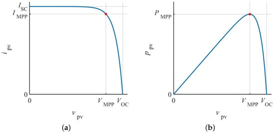
Figure 1.
PV generator output characteristics: (a) I–V curve; (b) P–V curve.
A PV generator is typically characterized by four important measures as indicated in Figure 1: , , , and . The MPP is represented by the values of and since the multiple is equal to the maximum power value . The is the open-circuit voltage that represents the highest PV output voltage under certain environmental conditions. The is the short-circuit current that represents the highest current of the PV output. Such parameters are widely used to design a safe and efficient PV system.
The curves and four parameters change with environmental conditions and the corresponding solar irradiance and temperature. An I–V curve tracer is expected to acquire a data set to recover the I–V and P-V curves under variable conditions. The deviation from the true values of , , , and is a critical measure of I–V tracing precision.
2.2. I–V Curve Tracer
The technology of I–V tracing should not be confused with the maximum power point tracker (MPPT), even though both share a common interest in the optimal operating point. The I–V curve tracer is often used for an offline test to diagnose faults and acquire characteristics of a PV generator’s output. I–V tracing needs to capture a whole range of operating points, from the open circuit to the short circuit. The MPPT operates in real-time generation to find the MPP and control the system at the optimal point, or within a narrow range, for the highest power output [8]. Thus, I–V tracing and MPPT are different technologies in terms of software algorithms, power conversion topologies, and performance indices.
The I–V curve of the PV generators should be acquired and plotted from open circuit to short circuit, as shown in Figure 1. The principle of I–V curve tracers can be illustrated by an equivalent circuit, as demonstrated in Figure 2a. The load resistance, R, is expected to vary smoothly from ∞ to 0 , namely, the active load, representing the open-voltage and short-circuit conditions of the PV generator, respectively [9]. A sensing system is required to acquire and record the paired variable ( and ), synchronized with the variation in R. The recorded data set should be sufficient to plot the V curve and capture the MPP with high resolution. Thus, the tracer design includes two major subsystems: the data acquisition and the dynamic load.
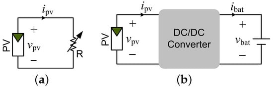
Figure 2.
Principle of I–V curve tracers: (a) equivalent circuit; (b) DC/DC-based solution.
One challenge lies on the load side, since the resistance is required to range from ∞ to 0 to produce a smooth plot of the V curves. A previous study summarized that the load can be produced by five approaches: variable resistive loads, capacitive loads, electronic loads, four-quadrant power supplies, and DC-DC converters [10,11,12,13]. Figure 3 shows the structure of the classification. Variable resistive loads follow the tracing principle, as shown in Figure 2a, but are difficult to implement in terms of physical constraints and high speed. Thus, the first four methods are commonly considered indoor solutions, regardless of speed, size, and cost, and are not suitable for outdoor tracers.
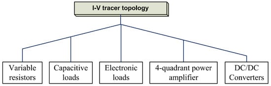
Figure 3.
Technologies for I–V curve tracers.
For outdoor applications, I–V curve tracers are typically portable and battery-powered. Previous studies have shown that the DC-DC converter method is superior to others for outdoor applications in terms of controllability, tracing speed, size, and cost [11,14]. Furthermore, the approach has the potential to recycle solar energy during the test when rechargeable batteries are applied as the power supply and load [12]. The block diagram, as shown in Figure 2b, demonstrates the concept of a battery-powered tracer using DC/DC converters for outdoor applications. The battery load and converter should produce the same effect as a variable load resistance, as demonstrated in Figure 2a. The question is which DC/DC topology is the best for this application.
3. DC/DC Topologies
Figure 2b shows the system construction for I–V curve tracers based on DC/DC converters. A prior study revealed that boost converters are ideal for PV power interfaces because of their simplicity and dynamic performance. However, either the buck or boost converter shows constraints in acquiring enough data sets to plot the complete I–V curve [11]. An investigation on buck–boost, Ćuk, SEPIC, and ZETA has been presented in the past; a comparison of the results is summarized in Table 1. The Ćuk and single-ended primary-inductor converter (SEPIC) show significant component counts, but the circuits favor fast dynamics for I–V traces. Thus, ref. [5] utilizes the Ćuk as the power interface, as it avoids impulsive current in both the input and output sections. ZETA is not an option due to its disadvantages.

Table 1.
Converter comparison for I–V curve tracers.
In the past, saving power switches was a trend in power converter development to save system costs. One example is the buck–boost converter developed from the cascade of a buck and a boost converter. The voltage inversion and shunt connection of the inductor saves one passive switch and one active switch, which was significant in the past. Similarly, the concept of the boost–buck converter evolved into the Ćuk topology by inverting the output voltage and connecting the interlink capacitor in series. The SEPIC was further developed to avoid voltage inversion between the input and output by the shunt connection of the output inductor. This development of Ćuk and SEPIC is based on the same cost-saving concept, using only one active switch and one passive switch for non-isolated DC/DC conversion.
Modern power electronics are developing increasingly high-performance, low-cost, and reliable-power semiconductors. Thus, the boost–buck converter can also be considered in developing I–V curve tracers for PV power systems, as shown in Figure 4a. The Ćuk and SEPIC can be considered as derivations from the boost–buck converter, as shown in Figure 4b and Figure 4c, respectively, for I–V curve tracing applications.
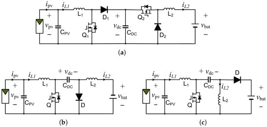
Figure 4.
DC/DC converters used for I–V curve tracing and battery loads: (a) boost–buck; (b) Ćuk; (c) SEPIC.
The interlinking capacitor is changed from a shunt connection in the boost–buck to a series connection in the Ćuk converter. This leads to the inversion of the voltage polarity from the input to the output, where . Thus, the active and passive switches in the series connection of the non-inverting topology can be removed. The diode in the boost–buck converter shunt connection needs to be changed to accommodate the negative voltage of the output in the Ćuk. The SEPIC was developed to correct the output voltage polarity and to recover the common ground. Again, it changes the output inductor from a series connection to a shunt connection to correct the voltage polarity. Therefore, the diode is applied in a series connection and rectifies the output voltage; .
4. Design and Modeling
This section introduces the design and a dynamic analysis of the three DC/DC topologies applied for I–V curve tracing applications.
4.1. Circuit Parameters
The passive components determine the system dynamics of in the front end, including and , as shown in Figure 4. The steady-state analysis leads to the parameters of and for all three DC/DC topologies, expressed by (1) and (3), respectively.
where represents the switching frequency and is the on-state duty ratio of the active switch that is determined by
where and are the steady-state values of and , where is in continuous conduction mode (CCM). The input capacitance is determined by
where and refer to the peak-to-peak ripples of the inductor current and PV voltage, respectively. Following the identical specifications of , , , , and , the ratings of and are the same for three topologies. The specified ripple levels in the nominal steady state can determine the parameters of and . For the boost–buck and Ćuk converters, the design of the output section can refer to the buck topology. For the SEPIC, the same design can be applied as a buck–boost converter for the 2nd stage.
4.2. Dynamic Analysis
One common advantage of the three topologies, as shown in Figure 4, lies in the input inductor, . With the , the capacitor-inductor (CL) circuit leads to a fast response at the PV side. The three topologies follow the same concept, assigning the boost topology at the input port. Thus, the response time should be the same among the three topologies if the parameters and are the same, which is determined by the ripple specifications of and . The averaging technique is commonly applied to derive system dynamics in power converters. Based on the CL circuit at the PV side, the averaged models are derived as (4) and (5). The current () is expressed as a function of in (6), which is typically represented by a single-diode model.
where , , , and represent the averaged values of , , , and , respectively. symbolizes the duty ratio for pulse-width modulation (PWM) when the active switch is turned on. The single-diode model for PV generators is nonlinear, representing the characteristics between and , as shown in Figure 1. Thus, the averaged models represented by the state variables and are nonlinear.
Dynamic resistance () is a way to linearize the relation between the output voltage and current of a PV generator [15], as shown in Figure 5. The resistance value shows the linearized relation between the PV voltage and current at the small-signal level, as expressed in (7). Although varies with the operating point along the I–V curve, the value can be considered a constant when an equilibrium is defined for a small-signal model, such as the MPP. Figure 5 also defines three important regions of PV output in terms of current source, power region, and voltage source, indicating the trend in . The resistance of is low in the voltage source region but high in the current source region.
where and represent the small-signal variations in and , as shown in Figure 5. A negative value of indicates that an increase in leads to a drop in , reflecting the I–V characteristics of PV generators.
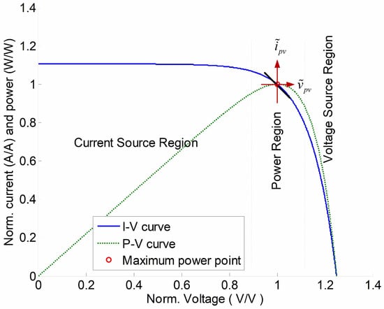
Figure 5.
Operational zones and small-signal definitions regarding , , and .
The small-signal model is written in the state-space format as (8), which includes two state variables: and . It is transferred to a single-input single-output (SISO) transfer function in (9).
where represents the small-signal perturbation of the duty ratio for PWM. symbolizes the small signal of the PV voltage, . In the SISO transfer function (9), the undamped natural frequency and damping ratio in (9) are derived as (10) and (11), respectively. The undamped natural frequency () is that at which a dynamic system oscillates freely without any energy dissipation or damping. Reflecting the response speed, a high indicates a fast system. The damping ratio () is an important parameter that describes how oscillations decay in a dynamic system. Both parameters are crucial for identifying and analyzing system dynamics.
where and refer to the capacitance and inductance, respectively, as indicated in Figure 4. is the dynamic resistance, as defined in (7). The DC gain () in (9) is expressed in (12), which is a negative value. A negative indicates that the increase in leads to a decrease in .
where refers to the averaged value of at steady state, which is considered a constant. Thus, the three topologies should demonstrate the same dynamic performance at the front end for the same PV generator in terms of speed and damping for I–V curve tracing.
5. Acquisition of Voltage and Current
Figure 6 shows a typical data acquisition structure that includes the sensing and conditioning steps. PV voltage and current are analog signals that are captured by sensing transducers. The acquired signal for transmission should be robust against electromagnetic interference, noise, and other disturbances. Therefore, signal conditioners are required to reduce the output impedance to output signals that are robust against noise and signal distortion. The frequency bandwidth in the sensing and signal-conditioning stages is high enough to capture all essential dynamics. The analog signals are sampled and converted to numerical values by analog-to-digital (A/D) units and recorded in a microcontroller. A portable device requires auxiliary power supplies (APSs) to source power from the battery and provide a regulated voltage to its microprocessor, signal conditioners, and communication devices.
Figure 6.
Block diagram of data acquisition for I–V curve tracers.
5.1. Sensing
The detection of the PV voltage, , can be achieved using a resistor divider to scale the voltage to a low level to match the voltage standard of the microcontrollers. The two resistors are marked as and in Figure 7. The sensing circuit is simple and low-cost.
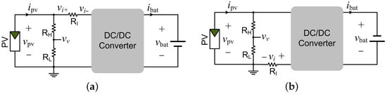
Figure 7.
Circuit for sensing voltage and current based on (a) common ground and (b) non-common ground.
There are two ways to measure DC current: Resistive current sensing (RCS) and a Hall effect transducer (HET). RCS is ideal for I–V curve tracers because of its accuracy and low cost. An accurate and high-bandwidth HET is relatively expensive. Another reason lies in the fact that outdoor I–V tracing takes only a very short time, milliseconds or microseconds; therefore, the concern of system efficiencies is a low priority. The implementations of RCS can be classified as low-side and high-side configurations.
In Figure 7 the shunt resistor is marked as in the series connection in the circuit to measure the PV output current, . The flowing current creates a differential voltage crossing , which is sensed to represent the current level according to Ohm’s law. When the sensing resistor is installed at the high side, the voltage potentials are measured as & , as shown in Figure 7a. The voltage difference between and is detected to represent . The advantage of high-side sensing is that the solution maintains a common ground between the input, output, signal conditioner, and microcontroller, and minimizes the ground disturbance.
Low-side current measurement places in the ground path. The advantage is clear: one signal, , is enough to represent the PV current when the PV negative terminal is treated as the common ground, as shown in Figure 7b. The drawback is that the system loses the common ground due to the placement of . In many cases, this makes ground-fault detection difficult, but this is not a concern for hand-held devices.
5.2. Signal Conditioning
Signal conditioners are required to amplify and strengthen sensing signals against noise; they are based on operational amplifiers. A simple signal conditioner is a voltage follower with high input impedance but low output impedance. It typically serves the purpose of the sensed signal, , which reflects , as shown in Figure 8. is transmitted through the signal conditioner to the analog-to-digital (A/D) unit for digital acquisition and recording.
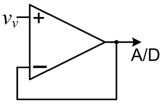
Figure 8.
Voltage follower for sensing PV generator voltage.
Signal amplification is typically required for RCS since is low in resistance and crossing voltage. Figure 9a demonstrates a typical high-side current-sensing circuit using operational amplifiers. The amplifier adopts a differential voltage between and and amplifies it to a higher level according to the gain setting resistors, and , which are equal in value to and , respectively. This is expressed in (13), where the single-end voltage, , is representative and proportional to . The voltage level of should be high to match the A/D unit and minimize noise during signal transmission.
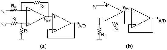
Figure 9.
Signal conditioning for sensing PV generator current using (a) differential amplifier and (b) voltage amplifier.
5.3. Auxiliary Power Supply
Auxiliary power supplies (APSs) regulate voltage to power a microprocessor, which is a common application, widely used in portable devices. The major consideration is the ground configuration for the signal conditioners to acquire the PV voltage and current.
The non-inverted output of the boost–buck and SEPIC is advantageous, where the batteries share a common ground through the negative terminals of the batteries, converter, and PV generator, as shown in Figure 4a,c. Such systems adopt the construction shown in Figure 7a for the acquisition of and . The RCS is based on the high-side configuration to maintain an equal ground. The power supply for the signal-conditioning circuit can be sourced directly from the battery or via a non-isolated power converter.
For Ćuk, the negative terminals of the PV generator and battery do not share a common ground due to the inverted voltage. An isolated power converter is required to share the same ground as the PV generator and supply power to the signal-conditioning circuits. High-side or low-side current sensing can be used to acquire thanks to the isolated power supply.
5.4. Comparison and Discussion on Converters
Table 2 summarizes the design and analysis based on the three topologies.
Table 2.
Topology comparison of I–V curve tracers.
The cascade configuration of the boost–buck makes the circuit complex, with a greater component count than the others. However, the topology provides flexibility to modulate the two active switches separately.
The difference between the Ćuk and SEPIC lies in the APS. The Ćuk relies on an isolated APS to deal with the polarity difference between the input and output. The SEPIC is flexible to adopt either non-isolated or isolated topologies for the APS. Where the battery-charging current is concerned, the Ćuk and boost–buck converters are superior to the SEPIC thanks to the inductor configuration for smoothing currents, as shown in Figure 4.
Regarding the system dynamics, all three are the same based on the analysis and modeling expressed in (9). The sensing and signal-conditioning circuits can be the same as well.
6. Tracing Algorithm
Section 3 discussed and analyzed that the three proposed topologies can support a fast response. The development of the control algorithm should support the hardware topology and enhance the performance. Thus, this section starts with the discussion of the tracing performance.
6.1. Tracing Performance
The tracing accuracy can be measured by three important points in the I–V curve. Table 3 defines the indices to measure tracing performance.
Table 3.
Tracing accuracy indices.
The open-circuit voltage of PV generators is the reference for the DC voltage rating in photovoltaic power systems. The deviation between the measured voltage and the actual value () is shown as in Table 3, where is the measured value of the open-circuit voltage. The short-circuit current provides the reference of the upper current limit for rating the over-current protective devices, cable, and DC disconnects. is defined as the performance index to indicate the precision of the measured value () compared to the actual current ().
The tracing accuracy of the maximum power point (MPP) is the most important since it represents the output power level. The concerns lie in the value and location of the MPP compared to the actual outputs. is defined as the precision index of the measured values in the terms and , compared to the actual MPP.
6.2. Control Operation and Strategy
The I–V curve trace can be achieved by varying the duty ratio from 0 to 100%, which causes the input impedance of an applied converter to range from ∞ to 0. There is a tradeoff, in that a large step size in the duty ratio leads to fast tracing but inaccuracy. On the other hand, a small step size results in slow tracing but better accuracy.
The dynamic analysis discovers the damping ratio (), expressed in (11). Studying the I–V curve reveals that shows high values when the operation is in the current region, as illustrated in Figure 5. The system damping ratio () is low in value, which leads to significant oscillation and increases the transient time. Thus, an optimal algorithm should be adaptive to follow the I–V curve and focus on performance indices.
The fixed step size (FSS) of the duty ratio is replaced by an adaptive step size (ASS) algorithm in the study of [5]. The sampling is intensified at the regions of the power and voltage source, as defined in Figure 5. This is achieved by assigning a small step size to the duty ratio. On the other hand, the step size is automatically tuned to be big to reduce the sampling points at the current source region, which is less important. The ASS approach improves the tracing accuracy, especially in the area around the MPP, which is the most important. It also avoids transient oscillations and makes the trace faster.
6.3. Evaluation and Comparison
The test is based on a 60-cell PV module with V, A, V, and A. A case study is conducted to demonstrate the tracing performance and is based on the standard test condition (STC). The STC is defined as a solar irradiance of 1000 W/m 2 and temperature of 25 ∘ C. Figure 10 illustrates the result of the proposed tracing algorithm compared to the fixed step size (FSS) method. The proposed algorithm intensifies the sampling points in the power and voltage regions, which are more important than the accuracy of the tracing in the current source region. The deviations in the open-circuit voltage and short-circuit current are the same between the FSS and ASS tracing algorithms. However, the deviation in the MPP is greatly reduced. Furthermore, the tracing time is significantly minimized since over sampling at the current source region is neglected.
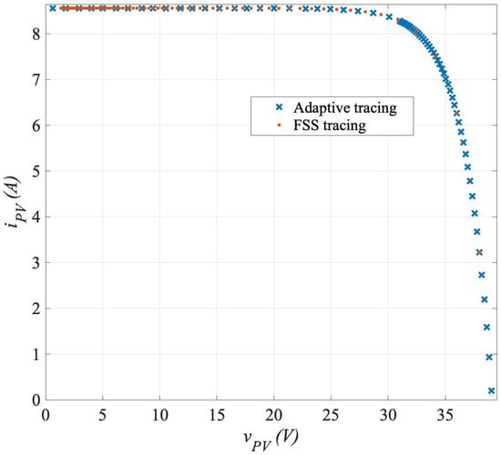
Figure 10.
Comparison of I–V curves at the STC traced by the traditional FSS (orange) and ASS algorithms (blue).
7. Conclusions
This paper provides an in-depth analysis and comparison study of I–V tracer technologies for PV power systems. Aiming for an outdoor test with natural sunlight, the instrument is defined as a portable and battery-powered device. The goal of the development includes fast tracing, accurate measurement, and energy recycling.
First, the article discusses three converter topologies that are suitable for the power interfaces to meet the requirements of this specific application. This reveals that the tracing dynamics are the same among the boost–buck, Ćuk, and SEPIC due to the CL circuit at the front end. The CL circuit design is based on the ripple specification and switching frequency. The advantages of the boost–buck and SEPIC lie in the non-inverted voltage polarity between the input and output. Ćuk wins for its output inductor configuration, which smoothens the current injected to the battery.
Second, a comprehensive study is presented including the sensing, signal conditioning, and ancillary power supplies (APSs). RCS technologies fit the current tracing application thanks to their low cost and accurate features. The signal conditioning is designed to amplify the sensing signal and make it robust against noise. The use of an isolated or non-isolated APS can be decided by the device requirements and the applied converter topology.
Third, the study recommends the ASS tracing method that is based on the nonlinear I–V curve of the PV output and performance indices. This technology is superior to the traditional FSS method in terms of speed and accuracy, especially for the most important point, MPP.
In summary, I–V tracers are important for diagnosing the degradation and malfunction of PV generators under various environmental conditions. This article is a valuable guide for academic research and industrial development.
Funding
This research received no external funding.
Data Availability Statement
No new data were created or analyzed in this study.
Conflicts of Interest
The authors declare no conflicts of interest.
References
- Spataru, S.; Sera, D.; Kerekes, T.; Teodorescu, R. Diagnostic method for photovoltaic systems based on light I–V measurements. Sol. Energy 2015, 119, 29–44. [Google Scholar] [CrossRef]
- Tavakoli, N.; Koelblin, P.; Saliba, M. Design and Development of a New Smart Portable I–V Tracer. IEEE J. Photovoltaics 2024, 14, 951–959. [Google Scholar] [CrossRef]
- Xiao, W. Photovoltaic Power System: Modeling, Design and Control; Wiley: Hoboken, NJ, USA, 2017. [Google Scholar]
- Triki-Lahiani, A.; Abdelghani, A.B.B.; Slama-Belkhodja, I. Fault detection and monitoring systems for photovoltaic installations: A review. Renew. Sustain. Energy Rev. 2018, 82, 2680–2692. [Google Scholar] [CrossRef]
- Zhu, Y. An Adaptive IV Curve Detecting Method for Photovoltaic Modules. In Proceedings of the 2018 IEEE International Power Electronics and Application Conference and Exposition (PEAC), Guangzhou, China,, 4–7 November 2022; IEEE: Piscataway, NJ, USA, 2018; pp. 1–6. [Google Scholar]
- Zhu, Y.; Xiao, W. Improved I–V Tracer for Detecting and Analyzing Photovoltaic Power Generators. In Proceedings of the 47th Annual Conference of the IEEE Industrial Electronics Society (IECON), Toronto, ON, Canada, 13–16 October 2021; pp. 1–7. [Google Scholar] [CrossRef]
- Huang, P.H.; Xiao, W.; Peng, J.C.H.; Kirtley, J.L. Comprehensive parameterization of solar cell: Improved accuracy with simulation efficiency. IEEE Trans. Ind. Electron. 2016, 63, 1549–1560. [Google Scholar] [CrossRef]
- Xiao, W.; Zeineldin, H.H.; Zhang, P. Statistic and Parallel Testing Procedure for Evaluating Maximum Power Point Tracking Algorithms of Photovoltaic Power Systems. IEEE J. Photovoltaics 2013, 3, 1062–1069. [Google Scholar] [CrossRef]
- De Riso, M.; Hassan, S.; Guerriero, P.; Dhimish, M.; Daliento, S. Enhanced Photovoltaic Panel Diagnostics: Advancing a High-Precision and Low-Cost I – V Curve Tracer. IEEE Trans. Instrum. Meas. 2024, 73, 1–10. [Google Scholar] [CrossRef]
- Sayyad, J.; Nasikkar, P. Design and Development of Low Cost, Portable, On-Field I–V Curve Tracer Based on Capacitor Loading for High Power Rated Solar Photovoltaic Modules. IEEE Access 2021, 9, 70715–70731. [Google Scholar] [CrossRef]
- Zhu, Y.; Xiao, W. A comprehensive review of topologies for photovoltaic I–V curve tracer. Sol. Energy 2020, 196, 346–357. [Google Scholar] [CrossRef]
- De Riso, M.; Matacena, I.; Guerriero, P.; Daliento, S. A Wireless Self-Powered I–V Curve Tracer for On-Line Characterization of Individual PV Panels. IEEE Trans. Ind. Electron. 2024, 71, 11508–11518. [Google Scholar] [CrossRef]
- Suresh, A.N.; Naveen, B.; Dusarlapudi, K. Design and Implementation of Cost-Effective PV String I–V and P-V curve tracer by using IGBT as a Power Electronic Load. In Proceedings of the 2024 6th International Conference on Energy, Power and Environment (ICEPE), Shillong, India, 20–22 June 2024; pp. 1–7. [Google Scholar] [CrossRef]
- Pereira, T.A.; Schmitz, L.; dos Santos, W.M.; Martins, D.C.; Coelho, R.F. Design of a Portable Photovoltaic I–V Curve Tracer Based on the DC–DC Converter Method. IEEE J. Photovoltaics 2021, 11, 552–560. [Google Scholar] [CrossRef]
- Xiao, W.; Dunford, W.G.; Palmer, P.R.; Capel, A. Regulation of photovoltaic voltage. IEEE Trans. Ind. Electron. 2007, 54, 1365–1374. [Google Scholar] [CrossRef]
Disclaimer/Publisher’s Note: The statements, opinions and data contained in all publications are solely those of the individual author(s) and contributor(s) and not of MDPI and/or the editor(s). MDPI and/or the editor(s) disclaim responsibility for any injury to people or property resulting from any ideas, methods, instructions or products referred to in the content. |
© 2025 by the author. Licensee MDPI, Basel, Switzerland. This article is an open access article distributed under the terms and conditions of the Creative Commons Attribution (CC BY) license (https://creativecommons.org/licenses/by/4.0/).