Hydroelectric Unit Fault Diagnosis Based on Modified Fractional Hierarchical Fluctuation Dispersion Entropy and AdaBoost-SCN

Abstract

The hydropower unit is the core of the hydropower station, and maintaining the safety and stability of the hydropower unit is the first essential priority of the operation of the hydropower station. However, the complex environment increases the probability of the failure of hydropower units. Therefore, aiming at the complex diversity of hydropower unit faults and the imbalance of fault data, this paper proposes a fault identification method based on modified fractional-order hierarchical fluctuation dispersion entropy (MFHFDE) and AdaBoost-stochastic configuration networks (AdaBoost-SCN). First, the modified hierarchical entropy and fractional-order theory are incorporated into the multiscale fluctuation dispersion entropy (MFDE) to enhance the responsiveness of MFDE to various fault signals and address its limitation of overlooking the high-frequency components of signals. Subsequently, the Euclidean distance is used to select the fractional order. Then, a novel method for evaluating the complexity of time-series signals, called MFHFDE, is presented. In addition, the AdaBoost algorithm is used to integrate stochastic configuration networks (SCN) to establish the AdaBoost-SCN strong classifier, which overcomes the problem of the weak generalization ability of SCN under the condition of an unbalanced number of signal samples. Finally, the features extracted via MFHFDE are fed into the classifier to accomplish pattern recognition. The results show that this method is more robust and effective compared with other methods in the anti-noise experiment and the feature extraction experiment. In the six kinds of imbalanced experimental data, the recognition rate reaches more than 98%.

1. Introduction

As the most stable and efficient green energy power generation method, hydropower generation is the key for countries to save energy and reduce emissions. Nevertheless, the rapid development of hydropower energy brings difficulties to maintaining its reliable operation. Hydroelectric generator units are the core of hydroelectric energy, and maintaining the security and stability of hydropower units is the primary principle. However, the complex environment and frequent switching conditions increase the probability of the failure of hydropower units. Therefore, finding a rapid and effective fault diagnosis method for hydroelectric generating units that utilizes vibration signals is of great practical significance for ensuring the safety and long-term operation of the equipment [1].

Existing research on fault diagnosis of hydroelectric generator units can be roughly summarized into two steps: feature extraction and pattern recognition. Feature extraction serves as the cornerstone of fault diagnosis, and the quality of extracted features significantly impacts the diagnostic outcomes. As a crucial metric for quantifying signal irregularity and complexity, entropy has been extensively utilized in mechanical system fault diagnosis [2,3,4]. Rajabi et al. successfully utilized permutation entropy to realize the fault diagnosis of rotating machinery [2]. However, multiscale permutation entropy (MPE) fails to account for the amplitude information in time series data, resulting in the loss of valuable information [5]. Lebreton et al. utilized multiscale dispersion entropy to quantify the complexity of signals from photovoltaic plant mechanical equipment, taking advantage of its sensitivity to signal complexity [4]. Multiscale dispersion entropy (MDE) overcomes the drawback of MPE in neglecting amplitude information but does not sufficiently consider the fluctuation of signals. Therefore, Azami proposed the multiscale fluctuation dispersion entropy (MFDE). MFDE considers the differences between adjacent signals and has the advantages of high stability, excellent detrending performance, and strong anti-interference ability [6]. However, the multiscale entropy method primarily focuses on fault information within the low-frequency segments of time series data, overlooking the high-frequency components [7]. Subsequently, the coarse process of MFDE is not sufficiently complete, and its capacity to adapt to high-noise environments is suboptimal [8]. Li et al. [9] utilized moving-average and moving-difference techniques to perform hierarchical decomposition of the raw time series, accounting for both high-frequency and low-frequency components at the same time. Compared to a single entropy value, fractional entropy exhibits higher sensitivity to signal evolution and stronger anti-noise performance, enabling the revelation of more details and information about the underlying system [10]. Otherwise, to address the issue of selecting the fractional order, inspired by the concept of Euclidean distance [11], this paper utilizes the Euclidean distance algorithm to optimize the order. Inspired by the aforementioned work, the modified fractional hierarchical fluctuation dispersion entropy (MFHFDE) is proposed.

Pattern recognition is a vital stage in diagnosing faults in hydroelectric generator units, essentially involving inputting fault data into a classifier to distinguish various fault categories. In recent years, artificial intelligence, founded on machine learning, has found application in hydroelectric generator unit fault diagnosis. References [12,13] have separately accomplished fault diagnosis in hydroelectric generator units utilizing convolutional neural networks and support vector machines. However, these models are limited in practical application for hydroelectric generator unit fault diagnosis due to their over-reliance on hyperparameters and long training times. As the latest model of stochastic parameter neural networks, the stochastic configuration network (SCN) has the advantages of few artificial parameters, short training times, and rapid convergence speed in disposing large-scale and high-dimensional data by virtue of its unique supervision mechanism and incremental network model [14]. However, SCN has weak generalization ability in situations with imbalanced signal quantities. In practical engineering scenarios, the amount of fault data for hydroelectric generator units is much less than normal data, resulting in an imbalance issue in the training data used for intelligent fault diagnosis. Accordingly, Freund proposed the AdaBoost ensemble classifier algorithm, which improves the accuracy of classifiers on imbalanced datasets by continuously updating the training sample weights and classifier weights, exhibiting advantages of simplicity and strong portability [15]. Based on the above theory, this paper uses SCN as the weak classifier and employs the AdaBoost ensemble algorithm to establish the AdaBoost-SCN strong classifier, overcoming the weak generalization ability of SCN under-imbalanced signal sample quantities.

In summary, targeting the multifaceted diversity of hydropower unit faults and the data imbalance issue, this paper introduces a hydropower unit fault diagnosis framework grounded in MFHFDE and AdaBoost-SCN. The key advancements and novel aspects are outlined below:

• The modified hierarchical entropy and fractional-order theory are incorporated into MFDE to boost its responsiveness to diverse fault signals and address the oversight of neglecting the high-frequency component of signals.
• Addressing the challenge of selecting the fractional order, the Euclidean distance is utilized to optimize the order, and a novel method for quantifying the complexity of time-series signals, termed MFHFDE, is introduced. The anti-noise performance and feature extraction capability of MFHFDE are analyzed, and it is demonstrated that MFHFDE surpasses traditional feature extraction methods such as HFDE, MFDE, and MDE.
• Utilizing the AdaBoost algorithm to assemble stochastic configuration networks, the AdaBoost-SCN strong classifier is established, which overcomes the problem of the weak generalization ability of SCN in the case of an unbalanced number of signal samples.
• The features extracted by MFHFDE are fed into the AdaBoost-SCN classifier. A novel fault diagnosis approach for hydroelectric units is proposed. The stability and superiority of this approach are confirmed via simulation experiments and contrasted against seven alternative models, such as HFDE-AdaBoost-SCN.

2. Related Theories

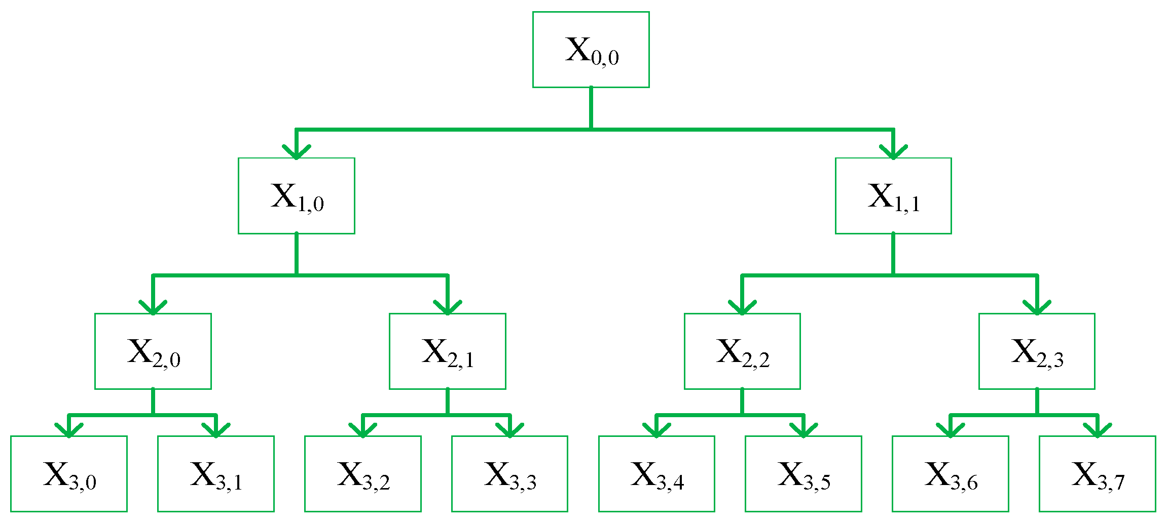
2.1. Hierarchical Fluctuation Dispersion Entropy

Hierarchical fluctuation dispersion entropy (HFDE) is a combination of fluctuation dispersion entropy and hierarchical entropy theory. It applies the moving-average and moving-difference methods to perform hierarchical decomposition on the original time series. The main steps for calculating the HFDE of a given time series $X=\{X(i),i=1,2,\dots N\}$ are as follows [16,17]:

Step 1:

For the original time series $X$, defines the operators $Q_0(x)$ and $Q_1(x)$ as:

$$\left\{\begin{array}{l}{Q}_0(x)={\displaystyle \frac{x_i+x_{i+1}}{2}}\\ Q_1(x)={\displaystyle \frac{x_i-x_{i+1}}{2}},i\in [1,N-1]\end{array}\right.$$

(1)

where N is the length of the time series; $Q_0(x)$ and $Q_1(x)$ represent the low-frequency and high-frequency components of the time series, respectively.

Step 2:

The matrix form of the operator $Q_l^k(l=0,1)$ for the k-th level can be represented as:

$$Q_l^k={\left[\begin{array}{l}{\displaystyle \frac{1}{2}} 0\mathrm{...0}{\displaystyle \frac{{(-1)}^l}{2}} 0\dots 0 0 0\\ 0{\displaystyle \frac{1}{2}} 0\mathrm{...0}{\displaystyle \frac{{(-1)}^l}{2}}\dots 0 0 0\\ \dots \\ 0 0 0 0 \dots {\displaystyle \frac{1}{2}} 0\mathrm{...0}{\displaystyle \frac{{(-1)}^l}{2}}\end{array}\right]}_{(N-2^k+1)\times (N-2^{k-1}+1)}$$

(2)

where k is the decomposition level. If k is too small, the frequency band division of the time series will not be detailed enough to obtain sufficient low-frequency and high-frequency components. If k is too large, the computational efficiency will be low. According to Ref. [18], we set k to 4.

Step 3:

Construct vectors $[v_1,v_2,\dots ,v_k]$ to represent non-negative integers:

$$e={\displaystyle \sum _{m=1}^k{2}^{k-m}{v}_m}$$

(3)

It can be observed that for a given integer e, there exists a unique $[v_1,v_2,\dots ,v_k]$ corresponding to it.

Step 4:

The hierarchical component $X_{k,e}$ at e-th node in the k-th level can be obtained as:

$$X_{k,e}=Q_{v_k}^k•Q_{v_{k-1}}^{k-1}\dots Q_{v1}^1•X$$

(4)

When the decomposition level is 3, the hierarchical decomposition process of the time series is illustrated in the Figure 1.

Step 5:

Map $X_{k,e}$ to $f=\{f(t),t=1,2,\dots ,2^k\}$ using the normal distribution function:

$$f(t)={\displaystyle \frac{1}{\partial \sqrt{2\pi }}}{\displaystyle \underset{-\infty }{\overset{X_{k,e}}{\int }}{e}^{\frac{-{(t-\mu )}^2}{2{\partial }^2}}dt}$$

(5)

where $f(t)\in (0,1)$, $\partial$, and $\mu$ represent the standard deviation and mean of the time series, respectively.

Step 6:

Each $f(t)$ is assigned to an integer within the range of 1 to c using a linear transformation, as shown below:

$$z(t)=R(c·f(t)+0.5)$$

(6)

where $z(t)$ represents the t-th element of the classified time series $Z=Z\{z(t),t=1,2,\dots ,2^k\}$, c denotes the number of categories, and $R(•)$ represents the integer part.

Step 7:

The embedding vector $Z_i^{m,c}$ is calculated according to the embedding dimension m and the delay d.

$$Z_i^{m,c}=[Z_i^c,Z_{i+d}^c,\dots Z_{i+(m-1)d}^{m,c}],i=1,2,\dots ,2^k-(m-1)d$$

(7)

Each embedding vector $Z_i^{m,c}$ is mapped to a fluctuation-based dispersion pattern ${\pi }_{v_0{v}_1\dots v_{m-2}}$.

Step 8:

The probability of each possible dispersion pattern ${\pi }_{v_0{v}_1\dots v_{m-2}}$ is calculated as follows:

$$p({\pi }_{v_0{v}_1\dots v_{m-2}})={\displaystyle \frac{N_{um}({\pi }_{v_0{v}_1\dots v_{m-2}})}{2^k-(m-1)\mathrm{d}}}$$

(8)

where $N_{um}({\pi }_{v_0{v}_1\dots v_{m-2}})$ represents the number of times the embedding vector $Z_i^{m,c}$ is mapped to each dispersion pattern ${\pi }_{v_0{v}_1\dots v_{m-2}}$.

Step 9:

The entropy value of the hierarchical fluctuation dispersion entropy can be obtained as:

$$HFDE(X,k,c,m,\mathrm{d})=-{\displaystyle \sum _{\pi =1}^{{(2c-1)}^{m-1}}p({\pi }_{v_0{v}_1\dots v_{m-2}})\cdot \ln (p({\pi }_{v_0{v}_1\dots v_{m-2}})})$$

(9)

2.2. Modified Fractional Hierarchical Fluctuation Dispersion Entropy

In 2014, Machado introduced Shannon entropy $I(p_i)=-\ln p_i$ as a zero-order function within the range of $D^{-1}I(p_i)=p_i(1-\ln p_i)$ and $D^{-1}I(p_i)=-1/p_i$ [19]. Inspired by this idea, HFDE was extended to the fractional domain, called FHFDE. The fractional hierarchical fluctuation dispersion entropy of a time series $X=\{X(i),i=1,2,\dots N\}$. can be calculated as:

$$FHFDE(X,k,c,m,\mathrm{d},\alpha )={\displaystyle \sum _{\pi =1}^{c^m}\left\{-\frac{p^{-\alpha }}{\Gamma (\alpha +1)}[\ln (p)+\psi (1)-\psi (1-\alpha )]\right\}}·p$$

(10)

where $\alpha$ represents the fractional order. When $\alpha$= 0, Equation (10) reduces to the hierarchical fluctuation dispersion entropy. $\Gamma$ and $\psi$ denote the gamma function and double gamma function, respectively. Currently, the selection of the order in fractional algorithms is mostly based on empirical knowledge or keeping other influencing parameters in entropy algorithms constant, discussing the impact of the order on the processing results [20,21]. However, this process is cumbersome and has limited scalability. The Euclidean distance optimization algorithm [22] has the advantages of short optimization time and strong portability. Therefore, considering these factors, the Euclidean distance is introduced to optimize the fractional order.

The Euclidean distance is the distance between two points in Euclidean space. Using this distance, Euclidean space becomes a metric space. The Euclidean distance is used to describe the spatial gap between two samples, where a larger distance indicates a greater difference in sample values and a lower similarity between the samples, while a smaller distance indicates a higher degree of similarity between the samples [23]. The Euclidean distance formula in a two-dimensional space is given by:

$$d=\sqrt{{(x_2-x_1)}^2+{(y_2-y_1)}^2}$$

(11)

where d represents the Euclidean $(x_2,y_2)$ distance between points $(x_1,y_1)$, and by using the Euclidean distance to optimize the fractional order, the Euclidean distance between two pairs of feature entropy values is calculated. A larger distance indicates a lower similarity between the two sets of features under this parameter, implying better feature extraction effectiveness. Conversely, a smaller distance indicates poorer feature extraction effectiveness under this parameter.

2.3. Stochastic Configuration Networks

SCN is a novel neural network that restricts the range of input weights, biases, and other parameters through a supervisory mechanism, giving the SCN model universal approximation properties. The specific computation process of SCN is as follows [24]:

Step 1:

Set initial input weights and biases as follows:

$$\left\{\begin{array}{c}{\omega }_s=\lambda \times (2\times rand(n,T_{\max })-1)\\ b_s=\lambda \times (2\times rand(1,T_{\max })-1)\end{array}\right.$$

(12)

where ${\omega }_s$ and $b_s$ are the input weight and bias of the s-th hidden node, respectively, and $\lambda$ is the scaling factor for ${\omega }_s$ and $b_s$. $T_{max}$ represents the maximum number of nodes in the hidden layer.

Step 2:

Use the sigmoid function to activate neurons in each layer. When the hidden layer node is S − 1, the output of SCN is given by:

$$Z_{S-1}={\displaystyle \sum _{s=1}^{S-1}{\beta }_s}\cdot g_s({\omega }_s^T\cdot W+b_s)(S=1,2,3,\dots ,Z_0=0)$$

(13)

where ${\beta }_S$ represents the output weight of the s-th hidden node, $W$ is the input vector, and the network error $e_{S-1}$ can be calculated as follows:

$$e_{S-1}=Z-Z_{S-1}=[e_{S-1,1},e_{S-1,2},\dots ,e_{S-1,D}]$$

(14)

Step 3:

Introduce a supervisory mechanism to randomly assign input weights and biases for node S as:

$${〈e_{S-1,h},g_S〉}^2\ge b_g^2(1-r-{\mu }_S)‖e_{S-1,h}‖,h=1,2,\dots ,D$$

(15)

where $-b_g\le g\le b_g$, $R^{+}∍b_g$; r is the regularization parameter ranging from 0 to 1; μ_S = (1 − r)/S + 1; D represents the output dimension; $g_S$ is the output of the Sth hidden node.

Step 4:

Utilize the least squares method to calculate the hidden layer output weights $\omega$ and biases $b$:

$$[{\beta }_1,{\beta }_2,\dots ,{\beta }_L]=\arg \min {‖Z-{\displaystyle \sum _{j=1}^L{\beta }_j{g}_j}‖}^2$$

(16)

Refer to the principles of setting SCN hyperparameters in Ref. [25]; the scaling factor for input weights and biases is set as {0.5, 1, 5, 10, 30, 50, 100, 150, 200, 250}, and the regularization parameter is set as {0.9, 0.99, 0.9999, 0.99999, 0.999999}.

2.4. AdaBoost-SCN

AdaBoost is a notable ensemble learning technique proposed by Freund et al. Its adaptability stems from the fact that the weights assigned to samples misclassified by the preceding weak classifier are enhanced, whereas the weights allocated to correctly classified samples are reduced. Then, the updated weights of all training samples are used to train the next weak classifier. In each iteration, a new weak classifier is added, and the weak classifier is evaluated based on the training results. By setting the number of iterations or a sufficiently small error rate, the result is integrated into a strong classifier.

In this paper, SCN is used as the weak classifier to integrate the ensemble learning technique of AdaBoost. The steps of the AdaBoost-SCN algorithm are as follows:

①

Initialize the weights of training samples $D_1$ according to Equation (17) and set the number of weak classifiers M. Repeat steps ② to ⑤ for each round:

$$D_1=1/N$$

(17)

②

Train the training samples based on the current weights $D_m$ of training samples to obtain the current weak classifier $SC{N}_m$.

③

Use the weak classifier to classify the training samples and obtain the classification $SC{N}_m$ error $e_m$.

④

Calculate the weight coefficient ${\alpha }_m$ of $SC{N}_m$ based on the classification error $e_m$ as follows:

$${\alpha }_m={\displaystyle \frac{1}{2}}\ln {\displaystyle \frac{1-e_m}{e_m}}$$

(18)

⑤

Update the weights of the training samples $D_m$ based on the classification result of $SC{N}_m$.

⑥

Stop training after reaching the predetermined number of iterations. Generate the strong classifier by combining according to Equation (19):

$$f(x)={\displaystyle \sum _{m=1}^M{\alpha }_{m}SC{N}_m(x)}$$

(19)

where $f(x)$ is the strong classifier function.

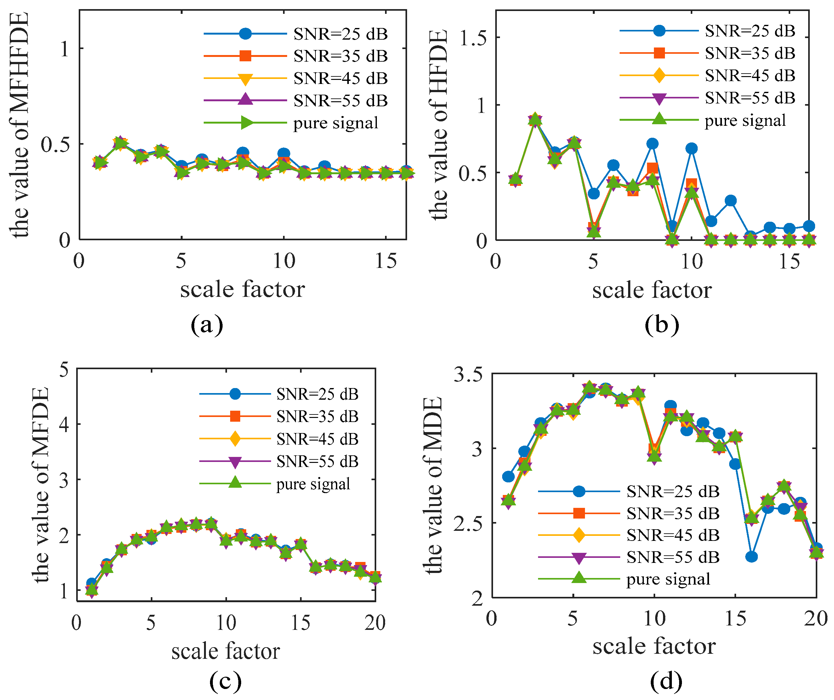
3. MFHFDE Performance Analysis

This paper comprehensively examines the performance of MFHFDE from two aspects: its noise immunity and ability to recognize different types of signals.

3.1. Analysis of MFHFDE’s Noise Immunity

The complex operating environment of hydroelectric units and the frequent changes in working conditions result in a large amount of noise in vibration signals. This requires MFHFDE to have high noise immunity. In this paper, the vibration fault signal caused by uneven guide vane openings is simulated as follows [26]:

$$\begin{array}{ll}S(t)=& 0.15\sin (\pi t)+0.21\sin (4.2\pi t)+\mathrm{0.0.9}\sin (33.4\pi t)+0.11\sin (58.4\pi t)\\ & +0.37\sin (100\pi t)+0.07\sin (200\pi t)+Z(t)\end{array}$$

(20)

where $S(t)$ is the simulated noisy vibration fault signal, and $Z(t)$ is Gaussian white noise; we used noise levels of 25 dB, 35 dB, 45 dB, and 55 dB. This paper compares and analyzes the distribution of the modified fractional-order hierarchical fluctuation dispersion entropy (MFHFDE), hierarchical fluctuation dispersion entropy (HFDE), multiscale fluctuation dispersion entropy (MFDE), and multiscale dispersion entropy (MDE) under different levels of noise. The results are shown in Figure 2.

From Figure 2, it can be observed that the HFDE, MFDE, and MDE of the vibration signals exhibit significant fluctuations, indicating that these three entropy models are more affected by noise and have weaker noise immunity. On the other hand, the MFHFDE shows relatively smaller and more stable fluctuations in the overall distribution of the vibration signals at any scale, indicating better noise immunity. The advantages, disadvantages, noise resistance and computing time of MPE, MDE, MFDE and MFHFDE are summarized in

Table 1. Performance comparison of entropy methods in fault diagnosis.

Method	Advantages	Limitations	Noise Robustness	Computational Cost	Reference
MPE	Simple computation	Ignores amplitude information	Low	1.0 s	[2]
MDE	Captures amplitude information	Neglects signal fluctuations	Medium	1.2 s	[4]
MFDE	Strong anti-interference, high stability	poor high-frequency adaptation	High	2.5 s	[6]
MFHFDE (Proposed)	Combines hierarchical decomposition and fractional entropy	Higher computational cost	Best	2.7 s

.

3.2. MFHFDE Feature Extraction Capability

As a feature extraction tool, a significant indicator for evaluating the performance of MFHFDE is its ability to effectively identify different types of signals. This paper evaluates the recognition performance of MFHFDE, HFDE, MFDE, and MDE on different datasets to assess their capabilities in recognizing different types of signals.

(1) 

Simulation Experiment 1

This section uses the rolling bearing fault data set of the bearing data center of Case Western Reserve University. The dataset consists of 10 types of bearing operating conditions: normal state, ball fault state, outer race fault state, and inner race fault state, with fault diameters of 0.1778 mm, 0.3556 mm, and 0.5334 mm, respectively (referred to as “NOR”, “BE1”, “OR1”, “IR1”, “BE2”,” OR2”, “IR2”, “BE3”, “OR3”, and “IR3”). The data is collected using two accelerometers installed at the drive end and fan end, with a sampling frequency of 12 kHz.

This article utilizes T-SNE (T-distributed Stochastic Neighbor Embedding, T-SNE) for visual analysis of the feature information extracted through MFHFDE, HFDE, MFDE, and MDE. The specific results are shown in Figure 3. It can be observed that the HFDE feature extraction results exhibit a significant overlap between the “BE2” state and the “IR2” state, as well as between the “Nor” state and the “OR1” state. The MFDE and MDE feature extraction results show many crossovers between ten fault states. For another thing, the MFHFDE-extracted features of the bearings show no overlap or confusion among different states, effectively distinguishing between the ten operational states of the bearings. Therefore, it can be inferred that MFHFDE demonstrates a feature extraction capability that surpasses the other three models. To replicate the real-world engineering settings and further explore the robustness and feature extraction capacity of the proposed method, white noise with a signal-to-noise ratio of 50 dB was introduced to the signals. As shown in Figure 3, even after the addition of noise, MFHFDE does not exhibit mixed or overlapping state features. In contrast, the HFDE, MFDE, and MDE algorithms yield more chaotic feature extraction results due to the presence of noise. This suggests that the MFHFDE algorithm still retains remarkable feature extraction capacities within high-noise settings.

(2) 

Simulation Experiment 2

In this subsection, the gear fault dataset from the University of Connecticut is used. The dataset consists of nine gear operating states: normal state, missing tooth fault, root crack fault, spalling fault, and five different degrees of sharpening faults (referred to as “NOR”, “MT”, “RC”, “Sp”, “Sh1”, “Sh2”, “Sh3”, “Sh4”, and “Sh5”). The sampling frequency is 12 kHz. Similarly, the MFHFDE, HFDE, MFDE, and MDE models are employed to extract features from the original dataset as well as the noisy dataset (SNR = 50 dB). T-SNE is utilized for the visual analysis of the extracted feature information, and the specific results are shown in Figure 4. It can be observed that, for both the original and noisy datasets, the MFHFDE extracts distinct features of confusion. It effectively distinguishes the nine gear operating states. On the other hand, the other three entropy algorithms exhibit overlapping state features in both cases and fail to completely differentiate the nine different gear operating states. This further confirms the excellent noise immunity and feature extraction capability of MFHFDE.

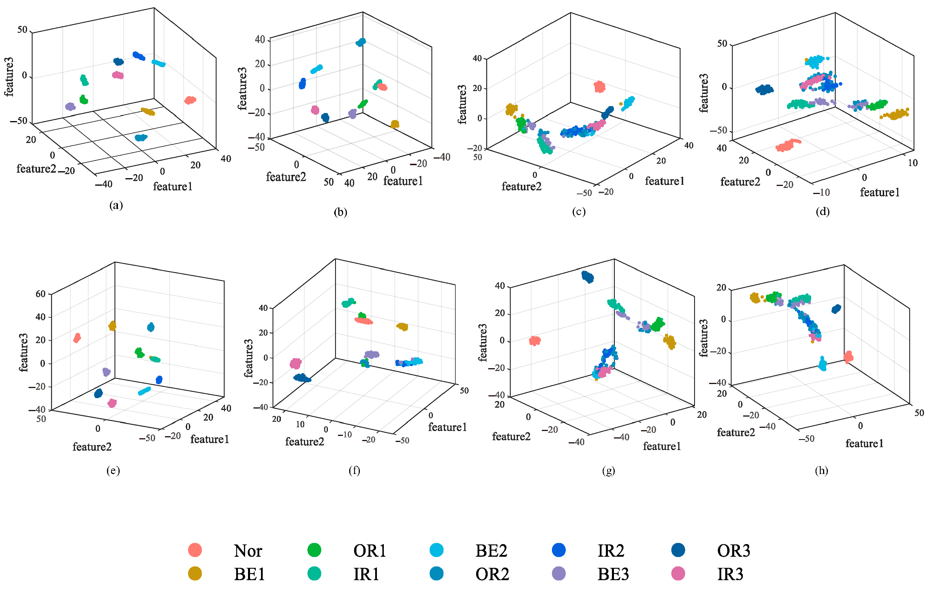
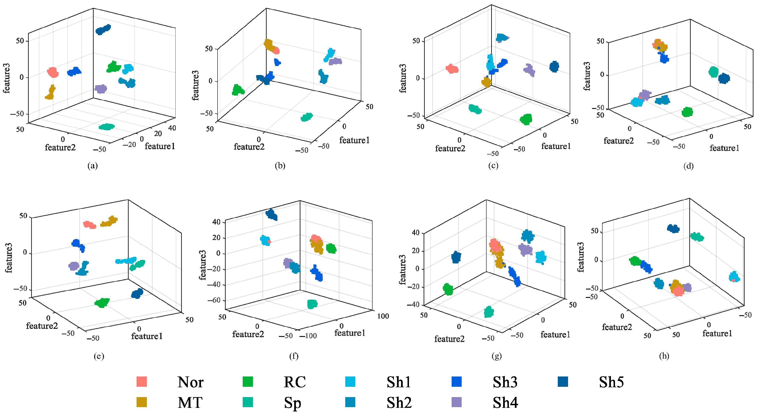
4. Experimental Analysis

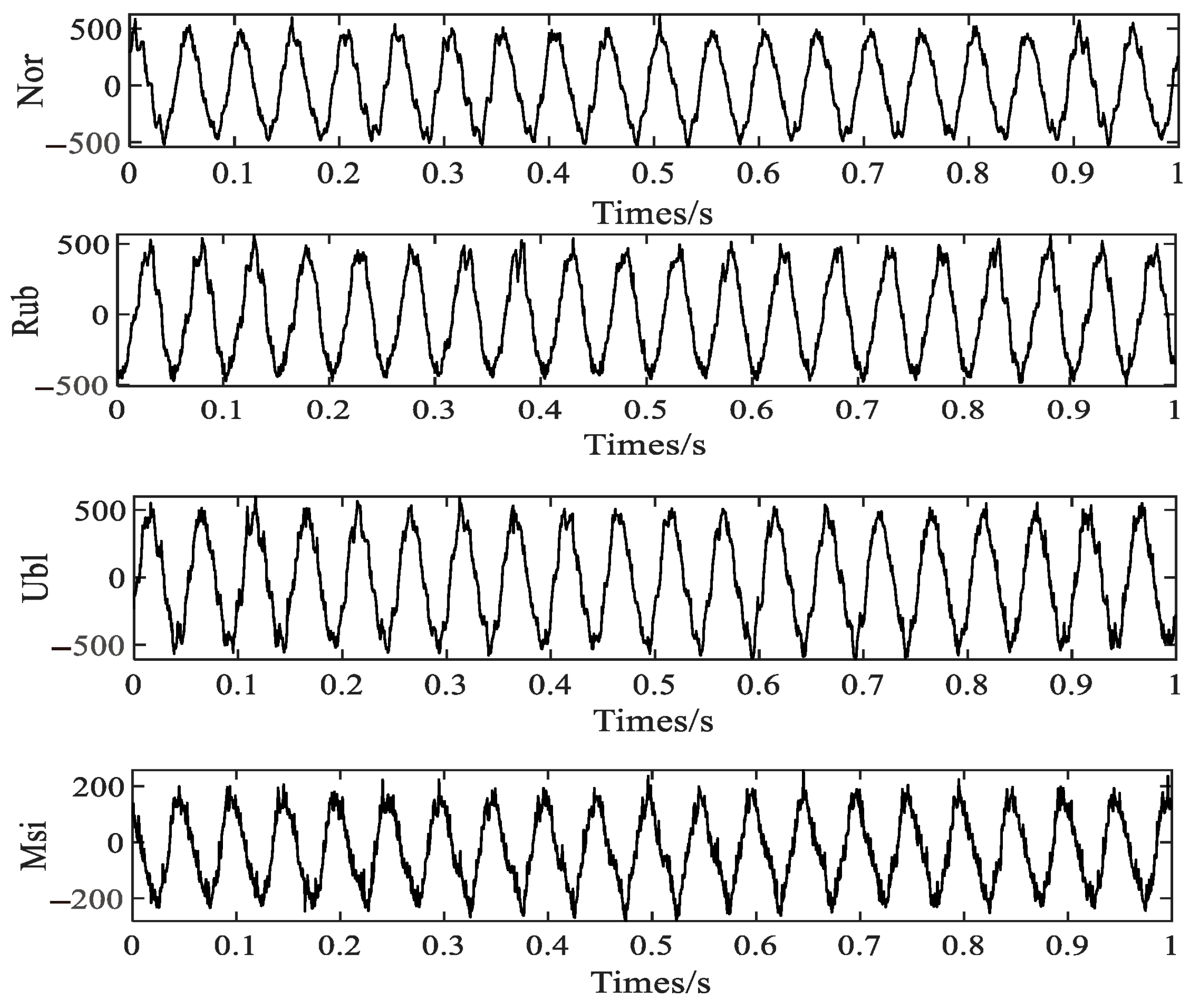
4.1. Vibration Data Acquisition on Rotor Test Bench

The test bench is made up of an HZXT-008H rotor rolling-bearing comprehensive fault simulation setup. It primarily consists of an electric motor, coupling, transmission shaft, data acquisition system, and computer, as depicted in Figure 5. By replicating varying degrees of damage faults at critical points, vibration signals are generated to mimic normal conditions and four common local damage faults: normal, unbalance, misalignment, and rubbing (abbreviated as “Nor”, “Rub”, “Ubl”, and “Msi”). The sampling rate is 2000 Hz, and a total of 600 datasets were gathered, each comprising 2048 sampling points, as illustrated in Figure 6.

Each set of collected data is sampled and divided into six imbalanced datasets using the sliding window sampling method for experimental analysis, as shown in

Table 2. Properties of a dataset.

Index	Dataset Abbreviation	Number of Faults Imbalance	Imbalance Ratio
1	Data1	12	10
2	Data2	24	5
3	Data3	36	3.33
4	Data4	72	2
5	Data5	90	1.33
6	Data6	120	1.00

. Table 2 displays the main characteristics of each dataset, including dataset abbreviation, number of faults, and imbalance ratio. The imbalance ratio represents the ratio of majority class samples to minority class samples, which in this experiment is the ratio of healthy samples to faulty samples.

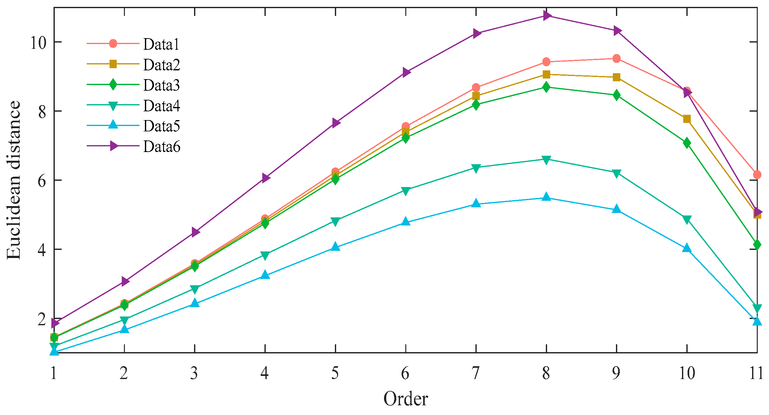
4.2. Selection of Euclidean Distance Optimization Algorithm Parameters

The selection of the fractional-order parameter α directly affects the MFHFDE feature extraction results. To determine the optimal value of α, the Euclidean distance optimization algorithm is used to optimize the parameters of MFHFDE during feature extraction for the six datasets. The results are shown in Figure 7. It can be observed that for all six datasets, the Euclidean distance is maximized when the fractional order is set to 0.3, 0.2, 0.2, 0.2, 0.2, and 0.2, respectively. This indicates that the best feature extraction performance is achieved at these fractional-order values. Therefore, the corresponding fractional-order values are selected for the six datasets to facilitate subsequent feature extraction and fault diagnosis.

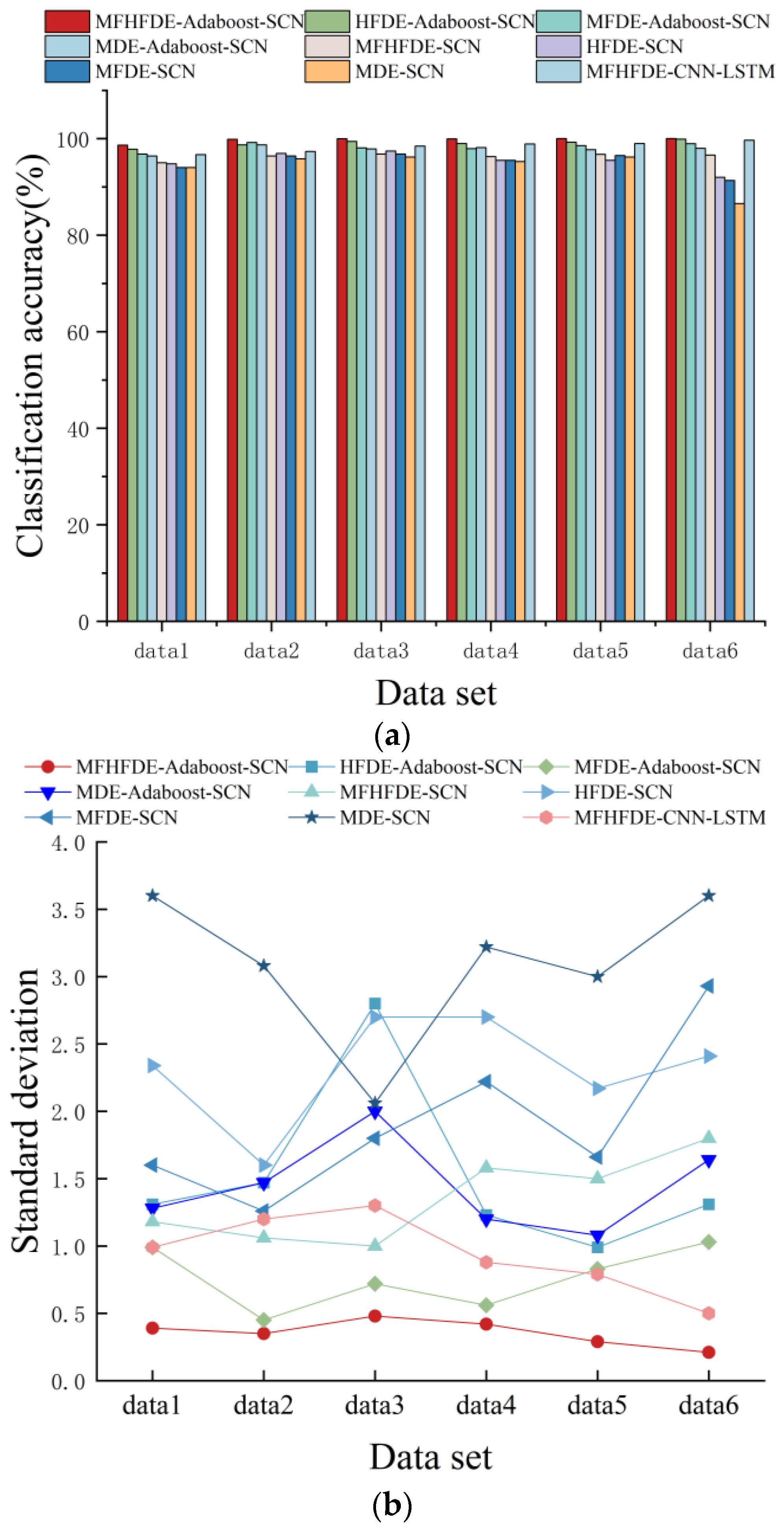
4.3. MFHFDE-AdaBoost-SCN Fault Recognition

We proportionally divide the sample data in each dataset into training and testing sets and input them into the fault diagnosis model based on MFHFDE-AdaBoost-SCN for fault recognition. We also introduce different fault diagnosis models for comparison. To eliminate the impact of random experiments on the final outcomes and assess the generalization capability of the proposed method, this study implemented five-fold cross-validation to evaluate the models. Each experiment was repeated 10 times, and the specific results are shown in Figure 8 and

Table 3. The diagnostic accuracy of the model. Emphasize the model proposed in this article in bold.

Model	Data1	Data2	Data3	Data4	Data5	Data6	Average Diagnosis Rate
MFHFDE-Adaboost-SCN	98.63	99.85	99.98	99.95	100	100	99.735	1
HFDE-Adaboost-SCN	97.8	98.7	99.43	99	99.28	99.88	99.015	2
MFDE-Adaboost-SCN	96.8	99.2	98.1	97.93	98.55	98.97	98.258	4
MDE-Adaboost-SCN	96.4	98.7	97.88	98.14	97.72	98	97.806	5
MFHFDE-SCN	95	96.42	96.8	96.28	96.75	96.6	96.308	6
HFDE-SCN	94.8	96.93	97.43	95.5	95.5	92	95.36	7
MFDE-SCN	94	96.42	96.8	95.5	96.5	91.33	95.092	8
MDE-SCN	94	95.8	96.2	95.25	96.2	86.55	94	9
MFHFDE-CNN-LSTM	96.67	97.33	98.45	98.88	99	99.68	98.335	3

. Compared to the other seven diagnostic models, the proposed model achieved the highest mean accuracy and the lowest standard deviation on all datasets. These results indicate that the proposed method has significant advantages in both diagnostic accuracy and algorithm stability. Furthermore, when comparing the feature extraction methods, the recognition rate of fault signals after using MFHFDE feature extraction exceeded that of the remaining three feature extraction techniques across all datasets. This indicates that the utilization of the fractional-order theory and the Euclidean distance optimization algorithm can better utilize fault information, addressing the issues of low sensitivity to signal evolution and difficult parameter selection in traditional entropy-based methods, thereby enhancing the diagnostic performance of the model. When comparing the classification methods, the AdaBoost-SCN diagnostic model outperformed the traditional SCN model in terms of diagnostic accuracy, indicating that the AdaBoost optimization algorithm effectively addresses the weak generalization capability of the SCN model in the case of imbalanced signal samples and improves the classification accuracy of the model. Moreover, among all the diagnostic results on the datasets, the MFHFDE-AdaBoost-SCN model exhibited better stability overall compared to the other seven models. This indicates that the proposed model can effectively learn the distribution characteristics of the signals, thereby improving the overall classification accuracy of imbalanced data.

5. Conclusions

This paper presents a hydroelectric unit fault diagnostic approach that integrates modified fractional hierarchical fluctuation dispersion entropy with AdaBoost-SCN. Firstly, based on the theories of hierarchical entropy, fractional order, and Euclidean distance, a new feature extraction tool called modified fractional hierarchical fluctuation dispersion entropy is introduced. Compared to traditional feature extraction methods, it has a higher noise immunity, superior feature extraction capability, and a better characterization of signal variations. Secondly, addressing the issue of data imbalance in hydroelectric unit fault diagnosis, the AdaBoost algorithm is used to integrate stochastic configuration networks and establish an AdaBoost-SCN strong classifier. The features extracted by MFHFDE are fed into the AdaBoost-SCN classifier, offering a novel fault diagnosis approach for hydroelectric units. Through simulation experiments and comparison with seven other models, including HFDE-AdaBoost-SCN, it is found that the proposed model achieves the highest diagnostic accuracy in six imbalanced datasets, with accuracies of 98.63%, 99.85%, 99.98%, 99.95%, 100%, and 100%. This validates that the MFHFDE-AdaBoost-SCN model is an effective hydroelectric unit fault diagnosis model with high diagnostic accuracy, providing a new approach for hydroelectric unit fault diagnosis and having practical significance.

References

1. Chen, F.; Zhao, Z.; Hu, X.; Liu, D.; Kang, Z.; Ma, Z.; Xiao, P.; Yin, X.; Yang, J. Enhancing the safety of hydroelectric power generation systems: An intelligent identification of axis orbits based on a nonlinear dynamics method. Energy 2025, 324, 135864. [Google Scholar] [CrossRef]
2. Rajabi, S.; Azari, M.S.; Santini, S.; Flammini, F. Fault diagnosis in industrial rotating equipment based on permutation entropy, signal processing and multi-output neuro-fuzzy classifier. Expert Syst. Appl. 2022, 06, 117754. [Google Scholar] [CrossRef]
3. Sun, Y.; Cao, Y.; Li, P.; Xie, G.; Wen, T.; Su, S. Vibration-based fault diagnosis for railway point machines using VMD and multiscale fluctuation-based dispersion entropy. Chin. J. Electron. 2024, 33, 803–813. [Google Scholar] [CrossRef]
4. Zhou, J.; Li, S.; Guo, J.; Wang, L.; Liu, Z.; Jin, T. Continuous hierarchical symbolic deviation entropy: A more robust entropy and its application to rolling bearing fault diagnosis. Mech. Syst. Signal Process 2025, 227, 112409. [Google Scholar] [CrossRef]
5. Li, Y.; Mu, L.; Gao, P. Particle swarm optimization fractional slope entropy: A new time series complexity indicator for bearing fault diagnosis. Fractal Fract. 2022, 6, 345. [Google Scholar] [CrossRef]
6. Azami, H.; Fernández, A.; Escudero, J. Multivariate multiscale dispersion entropy of biomedical times series. Entropy 2019, 21, 913. [Google Scholar] [CrossRef]
7. Chawla, P.; Rana, S.B.; Kaur, H.; Singh, K. Diagnosis of autism spectrum disorder using EEMD and multiscale fluctuation based dispersion entropy with Bayesian optimized light GBM. Multimed. Tools Appl. 2024, 83, 65341–65362. [Google Scholar] [CrossRef]
8. Tan, H.; Xie, S.; Liu, R.; Ma, W. Bearing fault identification based on stacking modified composite multiscale dispersion entropy and optimised support vector machine. Measurement 2021, 186, 110180. [Google Scholar] [CrossRef]
9. Li, Y.; Li, G.; Yang, Y.; Liang, X.; Xu, M. A fault diagnosis scheme for planetary gearboxes using adaptive multi-scale morphology filter and modified hierarchical permutation entropy. Mech. Syst. Signal Process 2018, 105, 319–337. [Google Scholar] [CrossRef]
10. Zheng, J.D.; Pan, H.Y. Use of generalized refined composite multiscale fractional dispersion entropy to diagnose the faults of rolling bearing. Nonlinear Dyn. 2020, 101, 1417–1440. [Google Scholar] [CrossRef]
11. Liberti, L.; Lavor, C.; Maculan, N.; Mucherino, A. Euclidean distance geometry and applications. SIAM Rev. 2014, 56, 3–69. [Google Scholar] [CrossRef]
12. Liao, G.-P.; Gao, W.; Yang, G.-J.; Guo, M.-F. Hydroelectric generating unit fault diagnosis using 1-D convolutional neural network and gated recurrent unit in small hydro. IEEE Sens. J. 2019, 19, 9352–9363. [Google Scholar] [CrossRef]
13. Reza, H.B.; Dragan, M.; Srete, N.; Dragicevic, T. Support vector machine-based islanding and grid fault detection in active distribution networks. IEEE J. Emerg. Sel. Top. Power Electron. 2019, 8, 2385–2403. [Google Scholar] [CrossRef]
14. Zhang, C.; Ding, S.; Zhang, J.; Jia, W. Parallel stochastic configuration networks for large-scale data regression. Appl. Soft Comput. 2021, 103, 107143. [Google Scholar] [CrossRef]
15. Wang, W.Y.; Sun, C.D. The improved AdaBoost algorithms for imbalanced data classification. Inf. Sci. 2021, 563, 358–374. [Google Scholar] [CrossRef]
16. Ma, J.; Li, S.; Qin, H.; Hao, A. Adaptive appearance modeling via hierarchical entropy analysis over multi-type features. Pattern Recognit 2020, 98, 107059. [Google Scholar] [CrossRef]
17. Zhou, F.; Gong, J.; Yang, X.; Han, T.; Yu, Z. A new gear intelligent fault diagnosis method based on refined composite hierarchical fluctuation dispersion entropy and manifold learning. Measurement 2021, 186, 110136. [Google Scholar] [CrossRef]
18. Li, W.; Shen, X.; Li, Y. A comparative study of multiscale sample entropy and hierarchical entropy and its application in feature extraction for ship-radiated noise. Entropy 2019, 21, 793. [Google Scholar] [CrossRef]
19. Machado, J.T. Fractional order generalized information. Entropy 2014, 16, 2350–2361. [Google Scholar] [CrossRef]
20. Wang, Y.; Shang, P. Complexity analysis of time series based on generalized fractional order dual-embedded dimensional multivariate multiscale dispersion entropy. Fractals 2021, 29, 2150048. [Google Scholar] [CrossRef]
21. Li, Y.; Tang, B.; Geng, B.; Jiao, S. Fractional order fuzzy dispersion entropy and its application in bearing fault diagnosis. Fractal Fract. 2022, 6, 544. [Google Scholar] [CrossRef]
22. Mesquita, D.P.; Gomes, J.P.; Junior, A.H.S.; Nobre, J.S. Euclidean distance estimation in incomplete datasets. Neurocomputing 2017, 248, 11–18. [Google Scholar] [CrossRef]
23. Zhou, R.; Wang, X.; Wan, J.; Xiong, N. EDM-fuzzy: An Euclidean distance based multiscale fuzzy entropy technology for diagnosing faults of industrial systems. IEEE Trans. Ind. Inform. 2022, 17, 4046–4054. [Google Scholar] [CrossRef]
24. Wang, D.; Li, M. Stochastic configuration networks: Fundamentals and algorithms. IEEE Trans. Cybern. 2017, 47, 3466–3479. [Google Scholar] [CrossRef]
25. Yang, S.; Ding, L.; Li, W.; Sun, W. Fishing risky behavior recognition based on adaptive transformer, reinforcement learning and stochastic configuration networks. Inf. Sci. 2024, 659, 120074. [Google Scholar] [CrossRef]
26. Xiao, H.; Zhihuai, X.; Dong, L.; Wenli, Z.; Hai, W.; Wenjun, J. Vibration fault identification method of hydropower unit based on EEMD-SDCC Ⅰ-HMM. Vib. Shock. 2022, 41, 165–175+230. [Google Scholar]
Figure 1. Hierarchical decomposition process when k = 3.
Energies 18 03798 g001
Figure 2. Entropy distribution under different signal-to-noise ratios: (a) MFHFDE; (b) HFDE; (c) MFDE; (d) MDE.
Energies 18 03798 g002
Figure 3. Visualization results of feature extraction of different entropy models under bearing data set: (a) MFHFDE (without adding noise); (b) HFDE (without adding noise); (c) MFDE (without adding noise); (d) MDE (without adding noise); (e) MFHFDE (SNR = 50); (f) HFDE (SNR = 50); (g) MFDE (SNR = 50); (h) MDE (SNR = 50).
Energies 18 03798 g003
Figure 4. Visualization results of feature extraction of different entropy models under bearing data set: (a) MFHFDE (without adding noise); (b) HFDE (without adding noise); (c) MFDE (without adding noise); (d) MDE (without adding noise); (e) MFHFDE (SNR = 50); (f) HFDE (SNR = 50); (g) MFDE (SNR = 50); (h) MDE (SNR = 50).
Energies 18 03798 g004
Figure 5. HZXT-008H sliding bearing comprehensive fault simulation test bench: (a) Test bench; (b) unbalance adjustment parts; (c) rubbing parts; (d) mass block; (e) sensor installation; (f) 16 channel data collector; (g) eddy current signal conditioner.
Energies 18 03798 g005
Figure 6. Different state signals collected by the simulation experiment platform.
Energies 18 03798 g006
Figure 7. Euclidean distance of various datasets at different orders.
Energies 18 03798 g007
Figure 8. The diagnostic results of different models under different datasets: (a) diagnostic rates (mean) for different models at different datasets; (b) diagnostic rates (standard deviation) for different models at different datasets.
Energies 18 03798 g008