A Deep Learning-Based Diagnostic Framework for Shaft Earthing Brush Faults in Large Turbine Generators

Abstract

Large turbine generators rely on shaft earthing brushes to safely divert harmful shaft currents to ground, protecting bearings from electrical damage. This paper presents a novel deep learning-based diagnostic framework to detect and classify faults in shaft earthing brushes of large turbine generators. A key innovation lies in the use of FFT-derived spectrograms from both voltage and current waveforms as dual-channel inputs to the CNN, enabling automatic feature extraction of time–frequency patterns associated with different SEB fault types. The proposed framework combines advanced signal processing and convolutional neural networks (CNNs) to automatically recognize fault-related patterns in shaft grounding current and voltage signals. In the approach, raw time-domain signals are converted into informative time–frequency representations, which serve as input to a CNN model trained to distinguish normal and faulty conditions. The framework was evaluated using data from a fleet of large-scale generators under various brush fault scenarios (e.g., increased brush contact resistance, loss of brush contact, worn out brushes, and brush contamination). Experimental results demonstrate high fault detection accuracy (exceeding 98%) and the reliable identification of different fault types, outperforming conventional threshold-based monitoring techniques. The proposed deep learning framework offers a novel intelligent monitoring solution for predictive maintenance of turbine generators. The contributions include the following: (1) the development of a specialized deep learning model for shaft earthing brush fault diagnosis, (2) a systematic methodology for feature extraction from shaft current signals, and (3) the validation of the framework on real-world fault data. This work enables the early detection of brush degradation, thereby reducing unplanned downtime and maintenance costs in power generation facilities.

1. Introduction

In modern power generation systems, large steam turbine generators are increasingly susceptible to damage caused by shaft voltages and bearing currents [1,2,3]. This vulnerability is exacerbated by the growing adoption of power electronic excitation systems and the implementation of flexible, dynamic operating regimes. Shaft voltages can originate from several sources, including electromagnetic induction, magnetic asymmetries, residual magnetism, and high-frequency harmonics introduced by static excitation equipment [1]. If these voltages are not effectively mitigated, they can induce circulating currents through the bearings, leading to electrical discharge machining (EDM), bearing pitting, lubricant degradation, and, ultimately, catastrophic mechanical failures.

Shaft earthing brushes (SEBs) play a critical role in mitigating these issues by providing a low-impedance path for the safe discharge of shaft currents to ground. These SEBs provide a low-impedance path to ground, preventing electrical discharge machining and pitting of bearing surfaces [1,2]. If an SEB deteriorates or fails, dangerous shaft currents can flow through bearings, leading to overheating and premature failure [2,3,4,5]. Undetected brush faults can result in costly unplanned outages of generators that are critical for grid reliability [3,4,6]. Therefore, the timely detection and diagnosis of SEB faults are of paramount importance for the safe and efficient operation of turbine generators [7,8].

The conventional maintenance of shaft grounding brushes often relies on periodic inspections or simple threshold alarms on shaft voltage and grounding current levels [7,8,9]. However, these traditional approaches may not detect subtle early-stage degradation or intermittent contact issues and often require expert interpretation, which can lead to missed faults or false alarms [2,7]. Recent review studies [10] have highlighted the need for more advanced monitoring techniques for shaft currents and voltages. Researchers have explored novel diagnostic methods; for example, the authors of [11] developed an electrostatic sensing approach to detect electrical discharge events in lubricated contacts, demonstrating alternative means to capture incipient faults. Meanwhile, data-driven approaches and machine learning methods have shown great promise in rotating machinery fault diagnosis [10,12].

Traditional diagnostic systems for generator shaft earthing rely heavily on basic time-domain indicators such as peak shaft voltage or current, which often lack the granularity to detect evolving fault mechanisms. In recent studies, including those referenced in [6,7,9], machine learning techniques have been applied to condition monitoring; however, these typically involve manual feature extraction. Such approaches depend on handcrafted features like harmonic content, statistical metrics, or predefined signal characteristics which require expert knowledge and are often sensitive to noise and machine-specific variations. In contrast, the deep learning framework proposed in this study employs a convolutional neural network (CNN) that learns meaningful representations directly from raw waveform data. This not only eliminates the need for manual feature engineering but also enhances the scalability and robustness of fault detection across different generator units and operating conditions. The proposed method thus provides a more autonomous and adaptable solution compared to earlier approaches.

Deep learning, a subset of machine learning based on multi-layer neural networks, has achieved remarkable success in fault diagnosis for various rotating machinery components such as bearings and gearboxes [9,11]. By learning directly from raw or pre-processed signals, deep learning models can outperform manual feature-based methods, especially in recognizing intricate patterns indicative of faults [9,11]. For instance, convolutional neural networks (CNNs) have been used to detect bearing faults from vibration signals with high accuracy, even under variable operating conditions [10,12,13]. These successes motivate exploring deep learning for diagnosing faults in generator shaft grounding brushes, which is a relatively under-investigated area compared to other machine components. Unlike prior works which mainly focus on bearing or motor faults [12,13,14], our framework addresses the unique challenges of SEB fault diagnosis. High-frequency measurements of shaft grounding current and voltage are leveraged, which carry diagnostic information about brush condition and apply time–frequency analysis to capture transient signatures of brush contact loss or degradation. A custom-designed CNN model is then trained to distinguish normal operation from various fault conditions automatically. The main contributions of this work are summarized as follows:

• Developed a dedicated novel diagnostic framework combining signal processing and deep learning to identify SEB faults. To the best of our knowledge, this is one of the first applications of CNN-based learning for shaft grounding brush fault diagnosis.
• Introduced a methodology to extract discriminative features from shaft current/voltage signals using time–frequency transforms. This approach highlights fault-related patterns (such as increases in high-frequency noise or intermittent surges) that are not evident in raw time-domain data.
• Validated the proposed framework on a fleet of large-scale turbine generators by emulating multiple SEB fault scenarios. The results show that our deep learning model can accurately detect brush faults and classify fault types, outperforming conventional monitoring methods. The findings demonstrate the potential of intelligent fault diagnosis for improving preventive maintenance in power generation.

The remainder of this paper is organized as follows: Section 2 describes the experimental setup and proposed methodology, including data acquisition, signal processing, and the CNN architecture. Section 3 presents the results of our fault diagnosis experiments and provides a discussion on the model’s performance. Section 4 details the fault detection accuracy on new test data and classification results for different fault types. In Section 5, we compare the proposed method with conventional fault detection approaches to quantify improvements. Section 6 (Key Findings and Discussion) interprets the results, emphasizing the significance of the findings and situating them in the context of existing practices. Finally, Section 7 (Conclusions) summarizes the work and suggests directions for future research in this domain.

Deep Learning for Rotating Machinery Fault Diagnosis

In the past 5–7 years, deep learning has gained prominence in diagnosing faults in large rotating machines (motors, generators, and turbines), often outperforming traditional signal processing and classical machine learning (ML) methods. Convolutional neural networks (CNNs), in particular, have shown the ability to automatically learn hierarchical features from minimally processed sensor data (vibrations, currents, etc.) [15,16]. For example, the authors of [17] developed a deep CNN for motor fault diagnosis that achieved high accuracy under noisy, variable loads without requiring manual noise filtering. The authors of [18] designed a dual-stream CNN to fuse time- and frequency-domain features of motor current signals, significantly improving the classification of motor faults compared to single-domain inputs. Likewise, spectrogram-based CNN models have been applied to insulation faults to recognize partial discharge patterns from time–frequency images, attaining high accuracy in distinguishing different discharge types [19]. These studies demonstrate that deep CNNs can automatically capture subtle fault signatures (e.g., harmonic distortions, transient patterns) that might be missed or require expert tuning in traditional approaches.

Beyond CNNs, other deep architectures have been explored. For instance, hybrid models and advanced variants incorporate attention mechanisms or recurrent layers converted raw signals to continuous wavelet transform images for a CNN to classify hydraulic pump faults while combined CNN and LSTM (optimized via Bayesian methods) for turbine fault diagnosis, outperforming standalone CNN or LSTM models [17,19]. Such approaches highlight the trend of leveraging deep learning’s automated feature extraction and multi-domain fusion to handle complex, multi-fault scenarios in rotating machinery.

Before the deep learning era, fault diagnosis relied heavily on manual feature extraction from sensor signals (vibration, acoustic, and current). Frequency-domain analysis (FFT spectra and envelope analysis) and time–frequency techniques (short-time Fourier transform (STFT) and wavelet transforms) were commonly used to reveal characteristic fault frequencies or patterns. These features would then feed into classical machine learning classifiers like Support Vector Machines (SVM) or decision trees. For example, the authors of [20] extracted wavelet packet features from vibration signals for bearing fault detection and achieved high accuracy using an SVM classifier. Similarly, STFT-based feature extraction has been applied to detect rotor unbalance (a mechanical imbalance). The authors of [20] demonstrated that using dynamic frequency-domain features (entropy measures of rotor response) combined with an SVM yields the accurate classification of different unbalance severity levels. These traditional pipelines can perform well but often require substantial domain knowledge—e.g., selecting the right decomposition level in a wavelet packet or the proper frequency band that reflects a specific fault.

Multiple studies in the late 2010s compared such model-based or feature-based methods with emerging deep learning models. The authors of [16] showed that a CNN using STFT spectrograms of motor signals outperformed manual FFT analysis for identifying faults like rotor imbalance. Traditional techniques like Motor Current Signature Analysis (MCSA) with expert-defined indices have been strong baselines for faults (e.g., detecting broken rotor bars or misalignment), but they struggle with noise and changing load conditions. Overall, classical approaches (FFT, wavelet, PCA + SVM, etc.) remain valuable for their interpretability and low computational cost, but they often require case-by-case tuning and may generalize poorly outside the conditions they were developed for [21].

Rolling element bearing defects have been a focal point for both traditional and DL methods. Early work used vibration spectrum features (e.g., kurtosis, resonance demodulation) to train SVM or ANN classifiers [21]. Recent deep learning approaches, however, learn bearing fault features automatically. For instance, the authors of [16] pioneered a data-driven CNN for bearing faults, achieving ~99% accuracy without manual preprocessing. More recently, researchers have even used motor current instead of vibration to detect bearing failures (avoiding extra sensors). The authors of [18] introduced a two-stream CNN combining raw current waveform and its frequency spectrum, which improved the detection of inner vs. outer race failures compared to using current features alone. Traditional methods like the wavelet-SVM reached 99–100% on lab datasets, but deep networks have shown better robustness to noise and load variations in bearing diagnostics [20,21].

Faults in insulation (e.g., stator winding degradation, partial discharges (PD)) are harder to detect via vibration, so electrical signal analysis is key. Conventional PD detection relies on phase-resolved discharge patterns (PRPDs) and expert rules, which are noise-sensitive [19]. Recent works leverage CNNs to classify PD spectrograms or PRPD images. The authors of [15] used a hybrid CNN-SVM to reach high precision in classifying sources of partial discharges. These deep models surpass traditional threshold-based PD detectors, especially under noisy conditions. The adoption of deep learning for insulation fault monitoring is still emerging, but early results show improved sensitivity to incipient faults and fewer false alarms compared to legacy systems.

Some specific faults, such as generator brush/shaft earthing brush (SEB) failures, have seen limited research. Traditionally these were monitored via threshold alarms on shaft voltage or current leakage levels. General studies on brush and slip-ring faults often relied on time-domain statistics or expert rules, which can miss subtle issues like partial contact or contamination. There is a clear research gap here: to date, few papers directly address SEB fault diagnosis with deep learning. However, the success of CNNs in analogous problems, e.g., detecting brush gear sparking via high-frequency current sensors, suggests potential [19]. It is reasonable to extrapolate that a CNN trained on voltage/current waveforms (transformed to time–frequency images) could learn the distinctive harmonic noise or discharge patterns of brush degradation (worn brush, floating contact, and dirt/oil interference), which are often very subtle in spectra. One recent study on wind turbine generators applied transfer learning to detect two faults, showing improved accuracy over a pure vibration analysis [15]. As more real-world data becomes available, we expect deep learning to be extended to these niche faults, directly comparing performance with the rule-based monitors currently in use.

2. Methodology

This section outlines the experimental design, signal processing techniques, and deep learning framework developed to diagnose shaft earthing brush (SEB) faults in large turbine generators. A combination of site-based testing and controlled fault condition simulations was conducted to acquire high-resolution voltage and current signals. These signals were then transformed into spectrograms using the Fast Fourier Transform (FFT) and were used as input for a convolutional neural network (CNN) classifier. The methodology encompasses the experimental setup, signal acquisition, fault simulation, spectrogram generation, model architecture, and training approach, providing a comprehensive pipeline for automated SEB fault detection and classification.

2.1. Experimental Setup

To develop and evaluate the diagnostic framework, various site experimental investigations were conducted on a fleet of large scaled-down turbine generator ranging from 200 MW to 846 MW (22 kV).

Shaft voltage and current measurements were carried out using a standardized setup, as illustrated in Figure 1. At the non-drive end (NDE) of the shaft, a high-impedance voltage brush was installed to sense the shaft’s electrical potential relative to ground. Simultaneously, a current-carrying brush was positioned at the drive end (DE), forming a low-impedance connection to ground via a precision shunt resistor (0.0496 Ω, rated at 150 A and 1100 W). The resulting voltage drop across the shunt was used to calculate the shaft grounding current. This arrangement provided effective grounding through the DE brush while enabling the concurrent acquisition of both voltage and current waveforms. Outputs from the voltage-sensing circuit and the shunt resistor were routed to a data acquisition system for synchronized waveform recording. A typical shaft earthing system comprises two main components:

• Voltage-Sensing Brush (Non-Drive End—NDE): This high-impedance carbon brush lightly contacts the generator shaft to monitor its potential relative to ground. While not designed to conduct substantial currents, it provides valuable diagnostic information about the shaft’s electrical behavior, enabling the detection of abnormal voltage conditions.
• Current Grounding Brush (Drive End—DE): This low-impedance, heavy-duty carbon or metal–graphite brush provides a direct path for shaft currents to flow safely to ground. It is responsible for discharging circulating shaft currents generated during normal operation or transient events, thereby protecting the bearings and insulation system from electrical stress.

2.2. Deep Learning-Based Fault Diagnosis Framework

The functional architecture of the deep learning-based shaft earthing brush (SEB) fault diagnosis system, designed in alignment with the operational characteristics of generator earthing fault mechanisms.

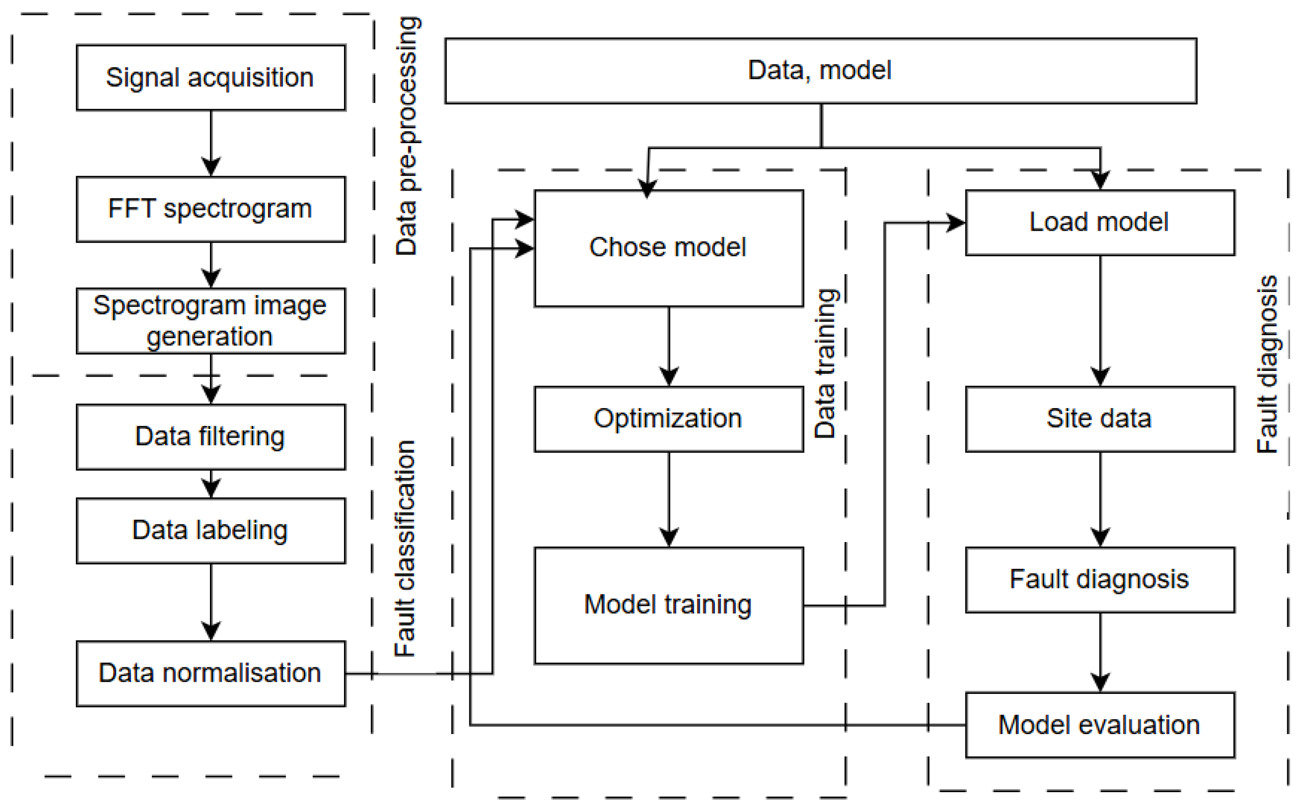
The proposed framework integrates real-time signal acquisition, spectral transformation, and deep learning-based classification to detect and distinguish between multiple SEB fault conditions in large turbine generators. As shown in Figure 2, the framework comprises four key functional modules: data pre-processing, fault classification, model training, and fault diagnosis.

In the data pre-processing stage, raw shaft voltage and current signals acquired from the field are subjected to a series of transformations to ensure suitability for neural network training. This includes signal filtering to remove electrical noise, data labeling based on known fault conditions (e.g., healthy, worn, floating, contaminated brushes), normalization to standardize input scales, and transformation into two-dimensional frequency spectrograms using the Fast Fourier Transform (FFT). These spectrograms encode the temporal and frequency-domain behavior of the signals, capturing harmonic distortions and transient anomalies that are characteristic of various fault conditions.

The fault classification phase is closely integrated with pre-processing and involves organizing the labeled and normalized spectrogram data for input into the convolutional neural network (CNN). As a data-driven system, the accuracy and reliability of the diagnostic model heavily depend on the quality of this pre-processed input.

The model training module provides capabilities for custom network design, hyperparameter tuning, the selection of optimization algorithms, and model checkpointing. These functionalities ensure a robust and generalizable training process capable of learning discriminative features for SEB fault detection. The trained CNN model is validated on unseen data to evaluate its diagnostic accuracy and avoid overfitting.

Finally, the fault diagnosis module encompasses model deployment, real-time monitoring, and the automated classification of new data. It supports the loading of the trained model, live inference, and the visualization of diagnostic results. The system also offers support documentation and user guidance to facilitate smooth operation and continuous fault monitoring in a live generator environment.

Collectively, this framework ensures a systematic, automated, and interpretable approach to SEB fault detection and classification, enhancing predictive maintenance capabilities and improving operational reliability in power generation systems.

2.3. CNN Based SEB Fault Diagnostic Process

The convolutional neural network (CNN)-based shaft earthing brush (SEB) fault diagnosis process is designed to systematically handle raw signal acquisition, pre-processing, model training, and online fault classification. This process is structured around the sequential flow of data and machine learning models, ensuring that each stage contributes effectively to the overall diagnostic accuracy and robustness of the system. The complete diagnostic workflow is illustrated in Figure 3.

The diagnostic process begins with the acquisition of raw voltage and current signals from shaft earthing brush monitoring systems installed on large turbine generators. These signals are typically characterized by noise and nonstationary features, necessitating robust pre-processing. In the data pre-processing phase, the signals undergo

• Noise filtering to remove high-frequency interference;
• Normalization to scale the data within a uniform range;
• Labeling based on operational conditions (healthy, floating, worn, and contaminated);
• Transformation into frequency-time spectrograms using Fast Fourier Transform (FFT) for spectral pattern encoding.

These spectrograms are saved as 2D images and serve as the input to the CNN model.

The model training phase uses the TensorFlow deep learning framework to implement a lightweight CNN architecture tailored for classifying spectral features associated with SEB fault conditions. Training includes

• Custom selection of convolutional and pooling layers;
• Specification of hyperparameters (e.g., learning rate, batch size, epochs);
• Optimization using the Adam optimizer;
• Evaluation using accuracy, confusion matrix, and loss curves.

Once trained, the model is validated on unseen test data to ensure generalization and robustness. During the fault diagnosis phase, the system loads the pre-trained CNN model and processes new incoming spectrograms generated from real-time online monitoring data. These are passed through the network to predict the fault class. The classification output is displayed via a graphical user interface (GUI), developed using the PyQt framework, which provides real-time visualization, result storage, and interpretability tools (e.g., t-SNE and UMAP visualizations from the penultimate CNN layer).

This architecture enables the end-to-end automation of fault diagnosis, minimizes manual interpretation, and supports condition-based maintenance strategies.

2.4. Fault Condition Implementation

To simulate real-world shaft earthing brush (SEB) fault scenarios under controlled conditions, the following procedures were followed:

• Baseline (healthy) condition: The brush properly contacts the shaft, with nominal grounding currents and negligible sparking.
• Floating voltage brush: The voltage-sensing brush at the non-drive end (NDE) is deliberately lifted, effectively creating an open circuit. Meanwhile, the current-carrying brush at the drive end (DE) remained in contact with the shaft to maintain grounding. This setup was intended to replicate a scenario where the voltage brush fails or is improperly seated. Both shaft voltage and current are recorded under this condition to assess the consequences of losing the primary voltage measurement path.
• Floating current brush: In this case, the main grounding brush at the DE was lifted, leaving only the high-impedance voltage brush in contact with the shaft. This simulated the loss of the main grounding connection. Shaft voltage and current are measured to understand how the system responds when the normal current discharge path is disrupted.
• Worn brush: The brushes used in these tests had previously been installed on a large turbine generator and had reached the end of their operational life. In line with standard maintenance practices, brushes are typically replaced when approximately 70% of their material has been consumed, leaving 30% of the usable length. This level of wear significantly affects contact stability and electrical conduction, providing a realistic representation of brush degradation in service. We conducted this test to examine how degraded brushes influence the reliability of shaft grounding.
• Oil and dust contamination: To simulate realistic contamination, a mixture of turbine seal oil and fine carbon dust is applied to the grounding brush. This condition replicates scenarios where oil leaks or airborne dust create insulating or abrasive layers on the brush-shaft interface. We captured shaft voltage and current data to evaluate how such contamination impacts electrical contact and grounding performance.

Each operating condition was run for several minutes under a steady machine speed and load, while continuously recording the shaft current and voltage signals. Fault conditions were repeated multiple times to capture sufficient data representing different stages of fault progression. The dataset was then labeled according to the condition (healthy or specific fault type) for use in training and testing the diagnostic model.

2.5. Signal Processing and Spectrogram Generation Using FFT

Effective fault diagnosis in shaft earthing brush systems requires accurate preprocessing of acquired signals to ensure consistent and reliable input to the diagnostic model. Shaft voltage and current signals were collected from high-impedance voltage-sensing brushes at the non-drive end (NDE) and low-impedance current grounding brushes at the drive end (DE), under both healthy and induced fault conditions—such as brush wear, oil/dust contamination, and floating contact.

To extract discriminative features in the frequency domain, raw time-domain waveforms were divided into overlapping segments (1 s duration with 50% overlap). This segmentation strategy preserved temporal continuity while capturing transient signal variations. Each segment was then subjected to a Fast Fourier Transform (FFT), converting 1D time-domain data into spectral representations that revealed frequency-domain signatures associated with various fault conditions. For example, elevated sub-synchronous components may indicate brush lift-off, while strong high-frequency harmonics often reflect contamination or arcing behavior.

The resulting magnitude spectra were normalized and mapped into 2D grayscale spectrograms resized to 256 × 256 pixels for compatibility with the CNN input layer. These spectrograms encode the evolution of frequency content in a form well-suited to convolutional learning, enabling the CNN to learn complex time–frequency patterns directly without manual feature engineering.

This preprocessing pipeline from time-domain acquisition to FFT transformation and spectrogram generation forms the foundation of the proposed deep learning-based classification framework. It enables compact yet expressive feature representation, improving both diagnostic sensitivity and generalization performance.

2.5.1. Rationale for FFT Selection

The Fast Fourier Transform (FFT) was selected as the spectral analysis tool based on several key considerations:

• Computational efficiency: FFT offers rapid computation, which supports scalable real-time deployment.
• Stationary signal behavior: The test signals were acquired under steady-state operating conditions. FFT, which assumes stationarity, was thus an appropriate choice.
• Interpretability: FFT-based spectral features such as harmonic peaks, DC offset, and spectral broadening are widely used in power system diagnostics, enhancing interpretability for practitioners.

Alternative methods like the short-time Fourier transform (STFT) and continuous wavelet transform (CWT) offer better time–frequency resolution but introduce additional computational complexity. These methods are typically more useful for analyzing non-stationary or transient behaviors, which were not the primary focus of this study. In contrast, FFT provided a suitable balance between performance, diagnostic clarity, and simplicity.

Furthermore, FFT-based spectrograms created a consistent, low-dimensional input format for the CNN, reducing overfitting risks given the relatively limited dataset. Future work may explore STFT or CWT representations in scenarios involving transient events or non-stationary behavior.

2.5.2. Spectrogram Generation Parameters

The FFT-based spectrograms were generated using the following configuration:

• Segment duration: 100 ms per segment (two full cycles at 50 Hz), capturing fault-induced harmonic features with adequate resolution.
• Sampling rate: 10 kHz, allowing harmonic analysis up to 5 kHz.
• FFT Details: A 1000-point FFT was applied to each segment without additional windowing, as the signals were quasi-stationary and edge effects were minimal.
• Image resolution: The normalized magnitude spectra were resized to 256 × 256 pixels to ensure uniform input dimensions for the CNN.

In summary, the FFT-based approach provided a computationally efficient and diagnostically meaningful method for transforming shaft voltage and current signals into a form usable by convolutional neural networks. The spectral features extracted were critical for identifying brush degradation mechanisms, enabling the accurate classification of fault types in large turbine generators.

2.6. Deep Learning Model Architecture

The deep learning model for fault classification utilizes a convolutional neural network (CNN) designed to process time–frequency spectrograms of shaft voltage and current signals derived via the Fast Fourier Transform (FFT). The CNN accepts dual-channel input images, each sized at 256 × 256 pixels, where one channel represents the shaft voltage spectrogram and the other the shaft current spectrogram. This two-channel format, analogous to RGB channels in conventional image processing, enables the model to learn joint spatial–frequency correlations across electrical parameters, thereby enhancing diagnostic accuracy.

As illustrated in Figure 4, the network architecture comprises two convolutional blocks. The first block includes a Conv2D layer with 32 filters (3 × 3 kernel), followed by a Rectified Linear Unit (ReLU) activation and a 2 × 2 max pooling layer. The second block applies a Conv2D layer with 64 filters (3 × 3 kernel), also followed by ReLU activation and a 2 × 2 max pooling operation. These convolutional and pooling layers work together to progressively extract high-level, abstract features relevant to brush fault detection while reducing spatial dimensionality and computational complexity. Max pooling, in particular, retains the most prominent features by selecting the maximum value within each 2 × 2 region, enhancing translational invariance.

Max pooling is employed after each convolutional layer using a 2 × 2 filter. This operation reduces the spatial dimensions of the feature maps by selecting the maximum activation within each pooling window. By preserving the most salient spatial features while discarding redundant or less informative activations, max pooling helps reduce the computational load and enhances the network’s robustness to small shifts or distortions in the spectrogram input. The two-stage convolutional-pooling sequence enables the progressive abstraction of frequency–temporal patterns associated with specific fault types.

The extracted feature maps are then flattened and passed through a dropout layer (dropout rate = 0.5) to reduce overfitting. This is followed by a fully connected dense layer with a softmax activation function, which outputs the predicted class probabilities across four fault categories: healthy, floating contact, worn brush, and oil/dust contamination.

The model is trained using the Adam optimizer with a learning rate of 0.001 and categorical cross-entropy loss, appropriate for multi-class classification tasks. Early stopping based on validation loss is employed to prevent overfitting. The dataset is split using an 80/20 stratified approach to maintain class balance in both training and test sets. To further improve model generalization, data augmentation techniques such as small time shifts and intensity scaling are applied to simulate realistic variations in signal acquisition.

2.7. Fault Classification Process

Summarizing the above, the proposed fault diagnosis process operates as follows:

• Continuously monitor the shaft grounding current and shaft voltage using appropriate sensors on the generator, and stream the data to the diagnostic system.
• Convert each time-domain segment into a time–frequency image (spectrogram or scalogram) that captures the signature of the brush condition.
• Input the image into the trained CNN model, which analyzes the patterns and outputs a predicted class label (healthy or specific fault type) along with a confidence score.
• If a fault class is detected with high confidence, trigger an alarm or maintenance alert. Otherwise, continue monitoring. The system can log results over time to track the evolution of brush condition.

This automated classification workflow enables the real-time or near-real-time monitoring of shaft earthing brush health. The computational requirements (for generating spectrograms and running the CNN) are modest and can be handled by an industrial PC or embedded GPU module at the generator site, making the framework feasible for online implementation.

2.8. Implementation Environment

To ensure the reproducibility and transparency of the proposed deep learning framework, this section outlines the software tools and libraries used for model development and evaluation. The entire diagnostic framework was implemented using Python 3.9, a widely adopted language in machine learning research.

Model training and inference were conducted using the PyTorch 2.0 deep learning framework, chosen for its flexibility and dynamic computation graph support. Key supporting libraries include the following:

• NumPy: Version 1.23.5, (https://numpy.org, accessed on 2 March 2024) for efficient numerical operations;
• Matplotlib: Version 3.7.1, (https://matplotlib.org, accessed on 2 March 2024) for visualization and plotting;
• SciPy: Version 1.10.1, (https://scipy.org, accessed on 2 March 2024) for signal processing routines;
• scikit-learn: Version 1.2.2, (https://scikit-learn.org/stable, accessed on 2 March 2024) for classical ML comparisons and evaluation metrics;
• Torchvision: Version 0.15.1, (https://pytorch.org/vision/stable, accessed on 2 March 2024) for preprocessing utilities and dataset handling.

This environment provided a robust foundation for the experimentation, visualization, and integration of both deep learning and signal processing techniques used in the study.

3. Data Processing

The accurate identification of fault conditions in shaft earthing brush systems is essential for the reliable operation of large hydrogen-cooled turbine generators. Each fault type introduces unique electrical disturbances that manifest in the shaft voltage and current signals. These disturbances can be effectively characterized through frequency-domain analysis using the Fast Fourier Transform (FFT), which converts time-domain waveforms into spectral representations, enabling the identification of frequency-specific fault features.

Such features form the basis for machine learning-driven classification, specifically using convolutional neural networks (CNNs), to automate the diagnosis of shaft earthing system anomalies. The fault signatures presented here were obtained through a combination of site-based experimental testing and historical data collection from multiple power stations operating hydrogen-cooled generators ranging from 200 MW to 846 MW at 22 kV. The primary objective was to evaluate shaft voltage and current behavior under both healthy and degraded brush conditions to generate labeled datasets suitable for training the diagnostic model.

4. Experimental Test Results and Analysis

The authors of [9] have observed through laboratory testing on a small synchronous generator rated at 20 kVA, 3000 rpm, and 50 Hz that each earth brush fault condition produces a distinct and measurable impact on shaft voltage and shaft current behavior. Below, we present the observed similar signal profiles performed on a large-scale generator for Power Station A under various shaft earthing brush fault conditions, compared against their respective healthy (baseline) states. These site-based measurements form a critical component of the dataset used to develop and validate the fault classification model. In addition to controlled experiments at Power Station A, similar tests were conducted at multiple other generating units across the utility’s fleet, including Power Stations B, C, D, E, F, and G, and similar characteristics were also observed. These tests involved the deliberate induction of brush faults such as floating (loss of contact), excessive brush wear, and contamination with oil and dust under varying machine load and operational conditions.

To ensure the robustness and generalizability of the deep learning-based diagnostic model, the site test results were further supplemented with historical condition monitoring data and waveform archives collected over several years. These datasets, acquired during routine maintenance inspections and post-incident investigations, include time-stamped shaft voltage and current recordings under both healthy and degraded brush conditions. The integration of this archival data enhanced the diversity of fault signatures in the training set, capturing a broader range of operating conditions, machine types, and environmental influences.

Together, this multi-source approach combining structured field experiments and historical records ensured the CNN model was exposed to rich and varied input patterns, enabling the high-fidelity classification of brush fault types across different generator units and operational contexts.

The summarized comparison in

Table 1. Power Station A baseline results versus all other earth brush fault conditions for both shaft voltage and current.

Parameter	Baseline	Floating Voltage Brush	Floating Current Brush	Worn Current Brush	Oil and Dust Contamination
$V_{rms\_peak}$	0.87 V	0.90 V	0.70 V	0.90 V	0.90 V
$V_{rms\_average}$	0.86 V	0.01 V	0.59 V	0.41 V	0.87 V
$V_{DC}$	0.01 V	0.17 V	0.13 V	0.07 V	0.12 V
$I_{rms\_peak}$	3.44 A	8.19 A	4.53 A	8.19 A	4.15 A
$I_{rms\_average}$	3.29 A	3.47 A	4.14 A	3.43 A	4.53 A

shows the Power Station A baseline results versus all other conditions for both shaft voltage and shaft current under different brush conditions (floating voltage brush, floating current brush, worn brush, and oil and dust contamination).

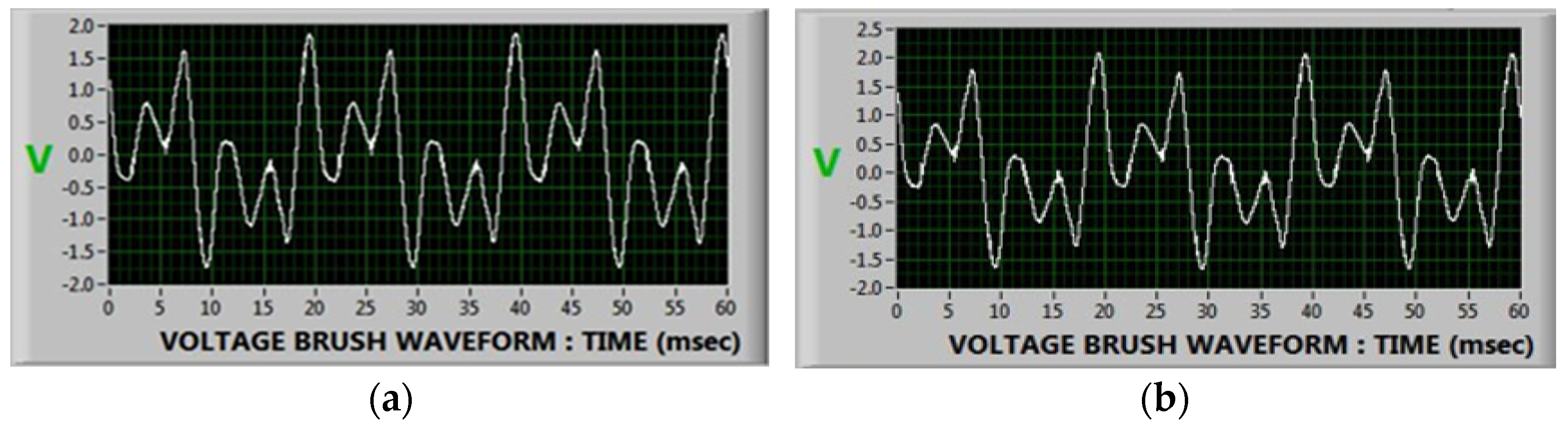
4.1. Power Station A Floating (Loss of Contact) Voltage Brush Test

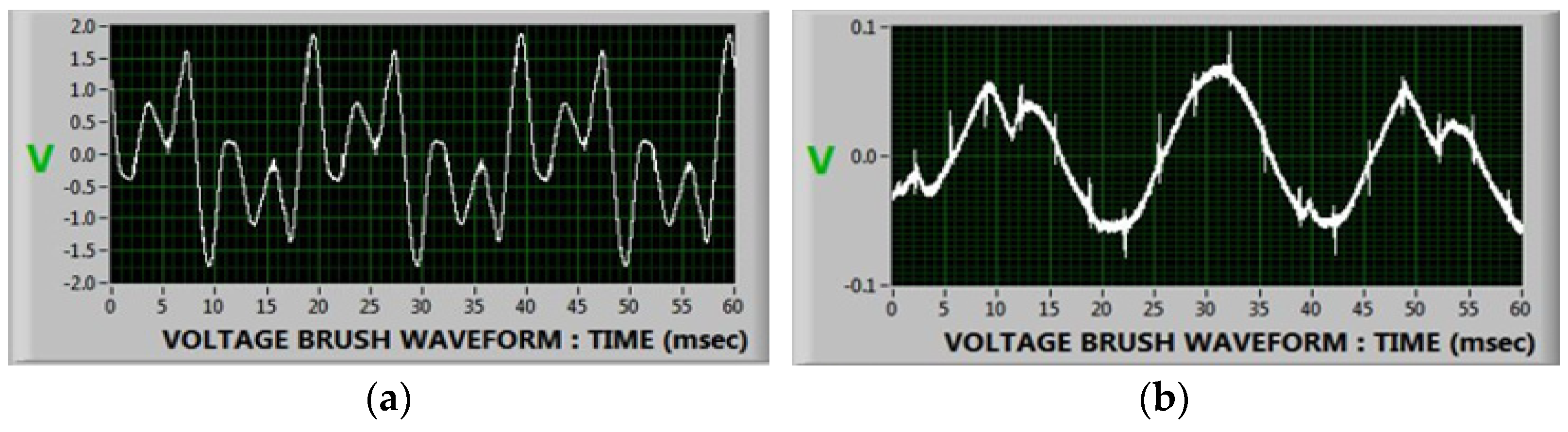
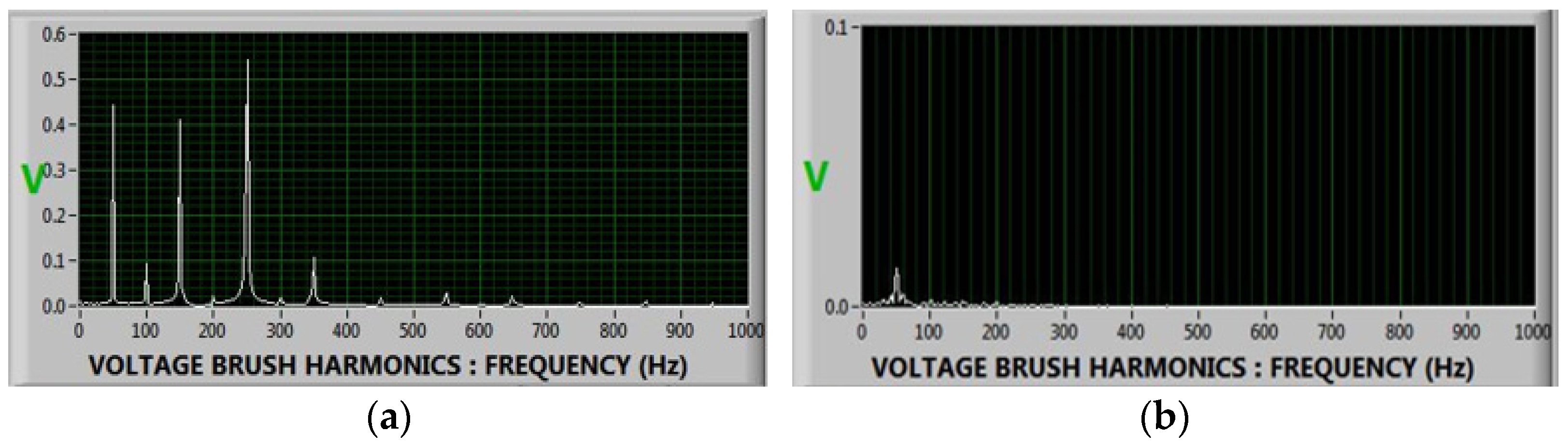
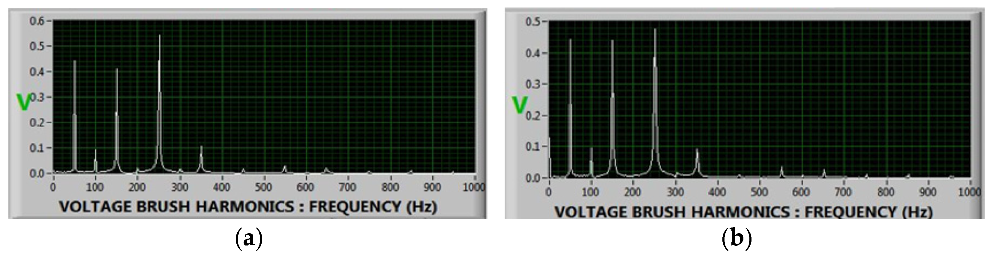
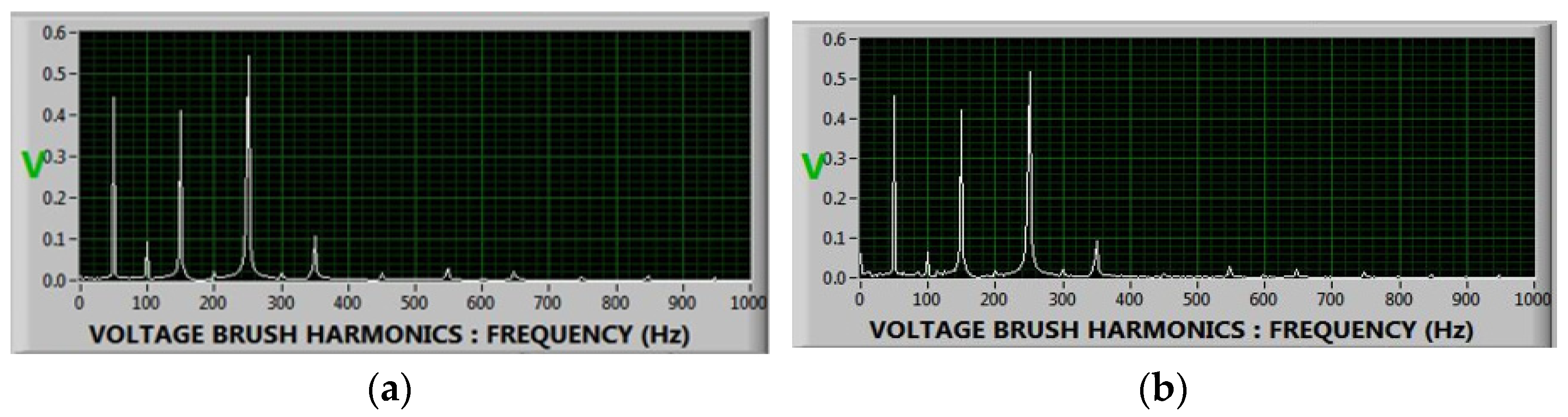
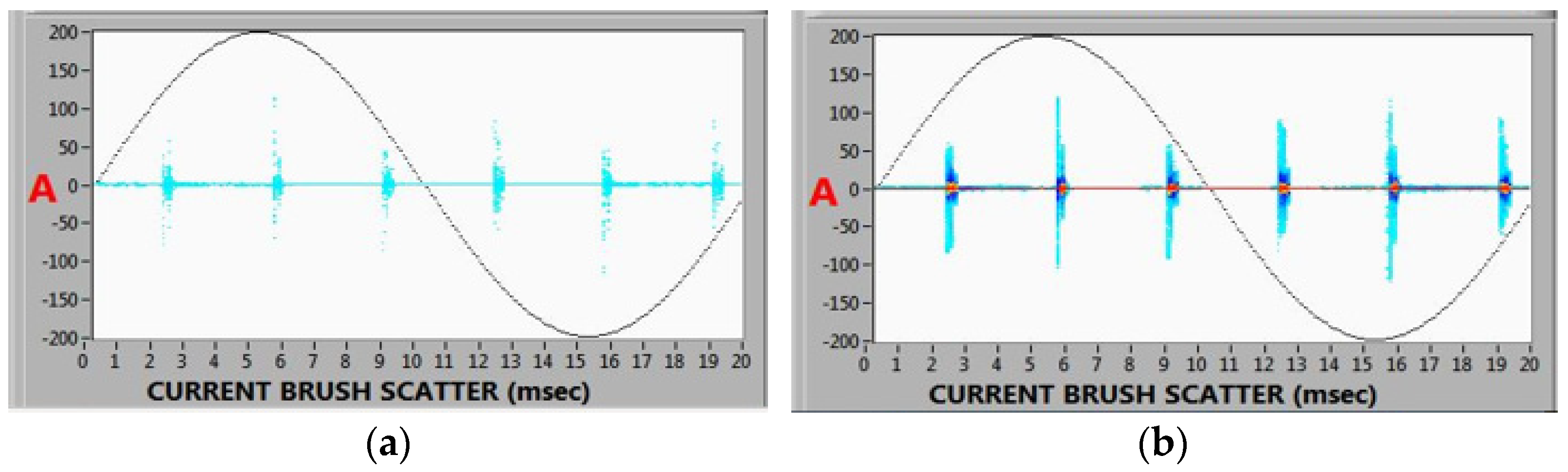
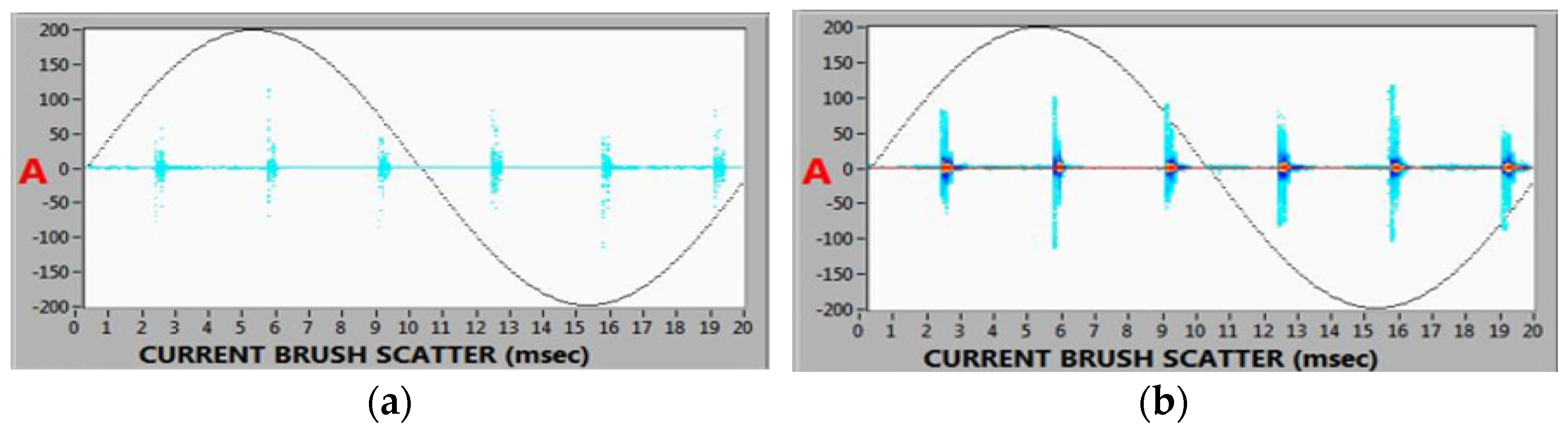
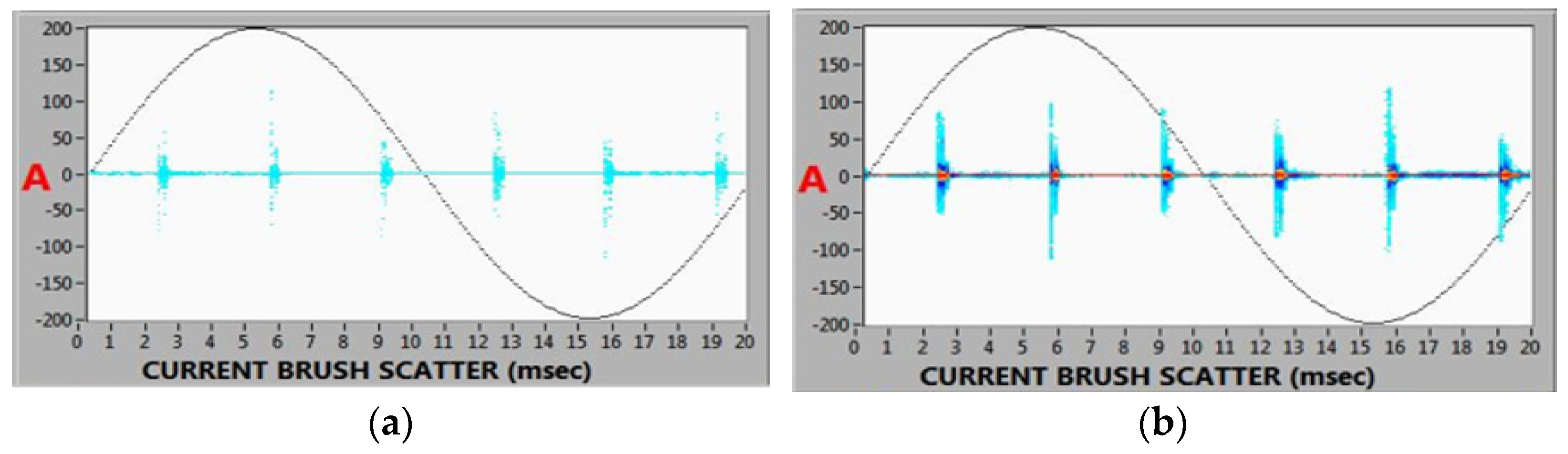
This condition simulates the scenario where the voltage brush loses physical contact with the shaft. The resulting voltage waveform (Figure 5b) displays erratic, low-amplitude signals in contrast to the stable sinusoidal pattern of the baseline (Figure 5a). The FFT spectrum (Figure 6b) reveals a substantial reduction in dominant harmonic components, indicating reduced coupling and altered capacitive discharge behavior. The corresponding current scatter plot (Figure 7b) exhibits increased amplitude variability and a more dispersed distribution compared to the baseline (Figure 7a), suggesting transient surges and a loss of current path integrity. In Figure 7b, the red regions denote areas of elevated current density, indicating transient spikes associated with floating brush conditions.

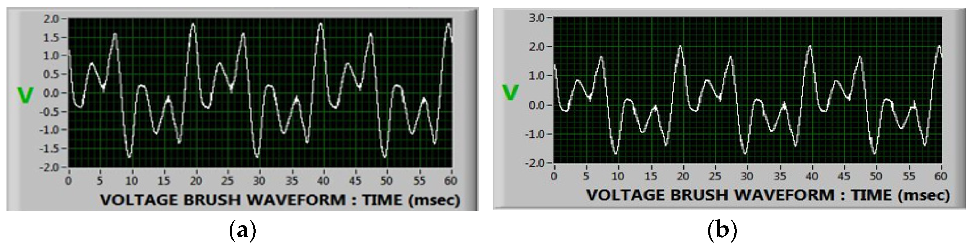
4.2. Power Station A Floating Current Brush (Loss of Contact) Test

In this test, the current brush was intentionally lifted to simulate a floating condition. As shown in Figure 8b, the shaft voltage waveform exhibits fluctuations and irregularities compared to the stable baseline in Figure 8a. The FFT response (Figure 9b) shows diminished harmonic energy and distorted frequency content, indicating impaired grounding. The scatter plot in Figure 10b illustrates dispersed current paths and the appearance of a red cluster, highlighting regions of high current density caused by transient instabilities associated with the floating current brush condition.

4.3. Power Station A Worn Current Brush

Brush wear is a progressive fault that degrades current conduction over time. The voltage waveform associated with worn brushes (Figure 11b) reveals increased noise and reduced waveform integrity compared to the baseline (Figure 11a). FFT analysis (Figure 12b) indicates elevated high-frequency content and spectral distortion, suggestive of arc-related emissions. The current scatter plot (Figure 13b) becomes more fragmented and less symmetrical, reflecting unstable brush-to-shaft contact.

4.4. Power Station A Current Brush Exposed to Oil and Dust

Contamination from oil and dust introduces non-uniform conductivity and noise in the shaft grounding path. As shown in Figure 14b, the shaft voltage waveform becomes distorted and inconsistent compared to the clean baseline in Figure 14a. FFT analysis (Figure 15b) reveals increased low-frequency harmonic content and energy spread, potentially being linked to partial discharges or intermittent arcing. The scatter plot in Figure 16b exhibits irregular amplitude excursions, indicating impaired current dissipation. The presence of red clusters highlights regions of elevated current density, attributed to transient spikes caused by contamination of the brush.

4.5. Comparative Analysis of Shaft Voltage and Current Fault Signatures Across Multiple Power Stations (A,B,C,D,E,F,G)

The shaft voltage RMS average across fault conditions scatter plot is shown in Figure 17. Key observations show that baseline voltage values are consistently high and stable across all stations.

The floating voltage brush (VB in blue diamond shape) exhibits near-zero voltage at all stations, highlighting full or partial contact loss. In contrast, the floating current brush (CB in purple) still retains some voltage, distinguishing the two fault types. The worn current brush (CB in a yellow triangle shape) and oil and dust (in red star shape) remain in the expected mid-to-high ranges.

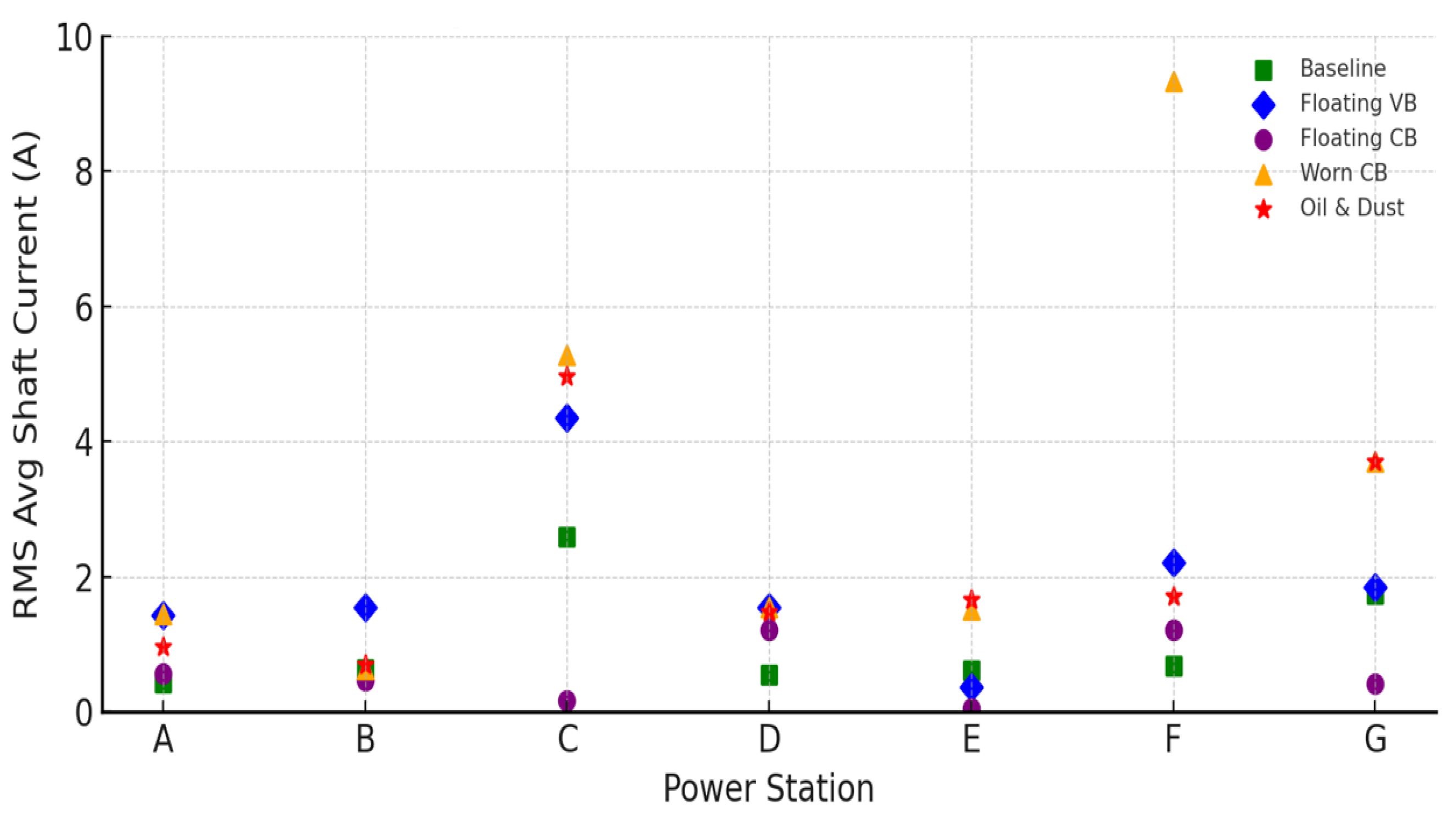
The shaft current RMS average across fault conditions scatter plot is shown in Figure 18. The floating VB shows elevated average shaft current at most stations, particularly Station C and F, indicating capacitive or stray path conduction despite the loss of voltage. The worn CB (orange) and oil and dust (red) generally show the highest average currents, aligning with partial conduction and contamination-based arcing.

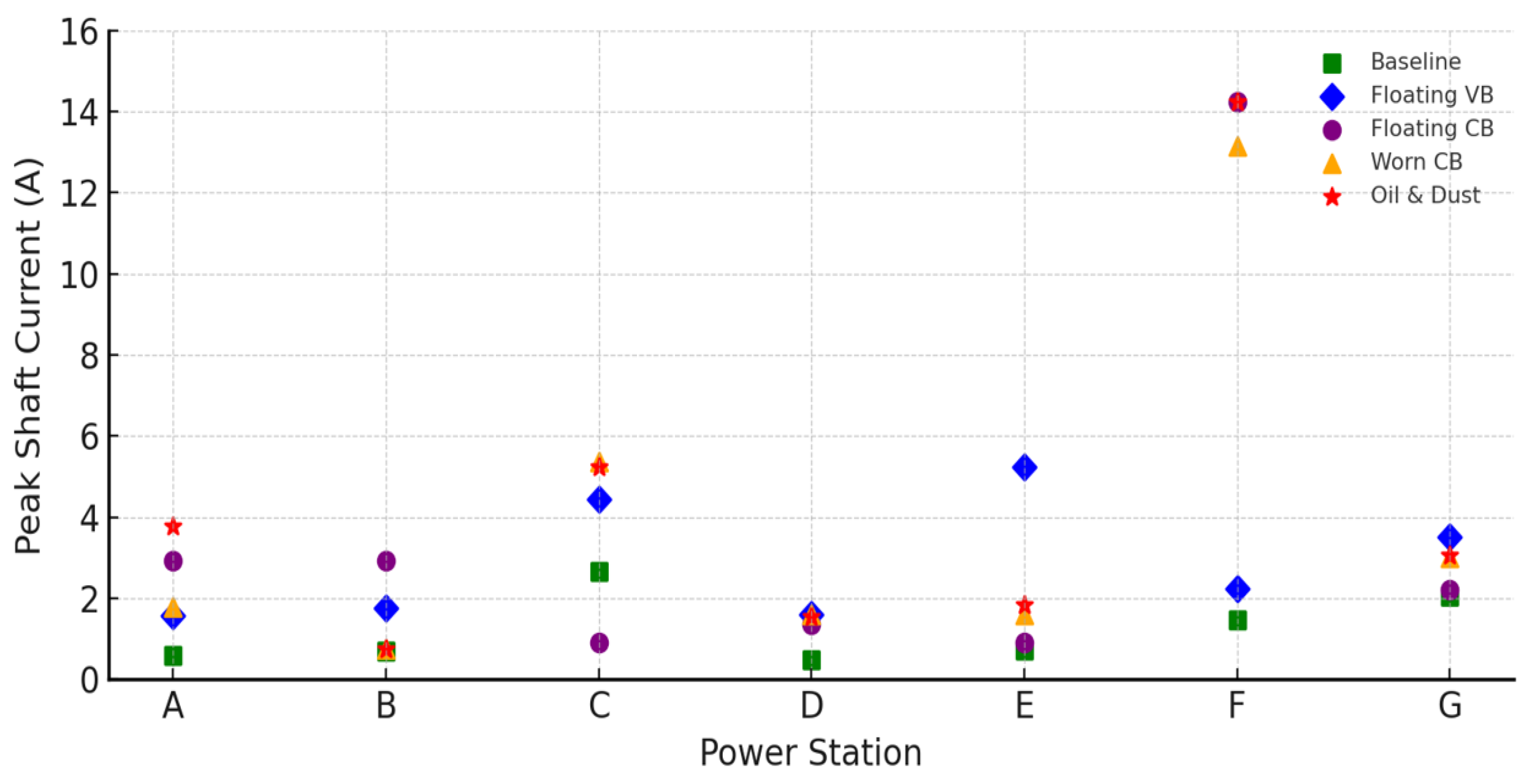
The peak shaft current across fault conditions scatter plot is shown in Figure 19. The floating VB again shows sharp surges, especially at Station E (5.24 A) and C (4.45 A), consistent with intermittent discharge. Peak shaft currents are most severe in the floating CB and oil and dust, particularly at Station F where values exceed 14 A.

Table 2. Synthesis and fault classification implications.

Fault Type	RMS Voltage Signature	RMS Current Signature	Peak Current Signature	Diagnostic Strength
Floating Voltage Brush	Strong voltage collapse; near-zero values	Near-zero or unstable	Low (intermittent conduction)	Easily detected via voltage collapse from shaft voltage waveform
Floating Current Brush	Stable voltage; minor asymmetry	Severe current drop or surges (station-dependent)	Highly variable and contact intermittency	Best detected through RMS current suppression combined with VDC trends.
Worn Brushes	Moderate voltage drop/stable	Elevated and erratic	Extreme surges at some stations	High average and peak currents combined with VDC trends; Needs multi-metric
Oil/Dust Contamination	Inconsistent voltage; mild DC increase	High sustained current and erratic	Severe peak discharges	Needs current focus and current scatter plots

presents a consolidated view of the key diagnostic signatures observed for common earthing brush fault types, compiled from RMS and peak signal analyses across multiple power station units. These patterns, established from experimental data and validated through site-level waveform interpretation, form the basis for fault classification and model training strategies. Each row links a fault condition to its electrical manifestation and diagnostic observability, facilitating the practical implementation of multi-metric fault detection frameworks.

5. Fault Detection Accuracy and Classification Results

The trained CNN model was evaluated on the independent test dataset to assess its fault detection accuracy and classification capability under realistic conditions. This test set contained data segments from all classes (healthy, brush wear, brush failure, or oil/dust contaminations) that the model had never seen during training or validation. The results demonstrate excellent performance of the diagnostic framework, confirming its potential for practical deployment.

5.1. Model Evaluation and Testing Protocols

To ensure a robust and reproducible evaluation of the CNN model, the dataset was partitioned using an 80%/20% train/test split strategy. Stratified sampling was employed to maintain class balance across both sets, ensuring that all four fault categories, namely healthy, floating brush fault, worn brush fault, and oil/dust contamination, were proportionally represented in the training and testing datasets. This mitigates the risk of model bias toward overrepresented classes and supports fair performance evaluation across all fault types.

Model performance was assessed using standard classification metrics, namely accuracy, precision, recall, and F1-score, computed on the test set. Additionally, confusion matrices were generated to visually represent the model’s classification behavior and class separability. The evaluation was performed across five randomized runs to account for variance in data splits, and the reported results reflect the average performance. This protocol ensures the validity of the conclusions drawn and supports reproducibility for future benchmarking.

5.2. Classification Results by Fault Types

The convolutional neural network (CNN)-based diagnostic model demonstrated high accuracy in identifying various fault conditions in the shaft earthing brush system. On the held-out test set, the model achieved an overall classification accuracy of 97.5%, with individual class performances as follows: 98% precision and 97% recall for the floating voltage brush, 95% precision and 94% recall for floating current brush, 97% precision and 98% recall for worn brushes, and 99% precision and 99% recall for oil/dust contamination. These results indicate that the model exhibits both high sensitivity to fault occurrences and a very low false alarm rate for healthy brushes.

Table 3. Classification results by fault type.

Fault Type	Precision	Recall	F1-Score
Floating Voltage Brush	0.98	0.97	0.975
Floating Current Brush	0.95	0.94	0.945
Worn Brushes	0.97	0.98	0.975
Oil/Dust Contamination	0.99	0.99	0.99

summarizes the classification performance metrics, including precision, recall, and F1-score, for each fault category. Notably, all F1-scores exceed 0.94, reflecting consistent and robust detection across all failure modes. The results confirm that the CNN is capable of capturing distinct diagnostic features from time–frequency representations of shaft voltage and current signals.

5.3. Confusion Matrix for Shaft Brush Fault Classification

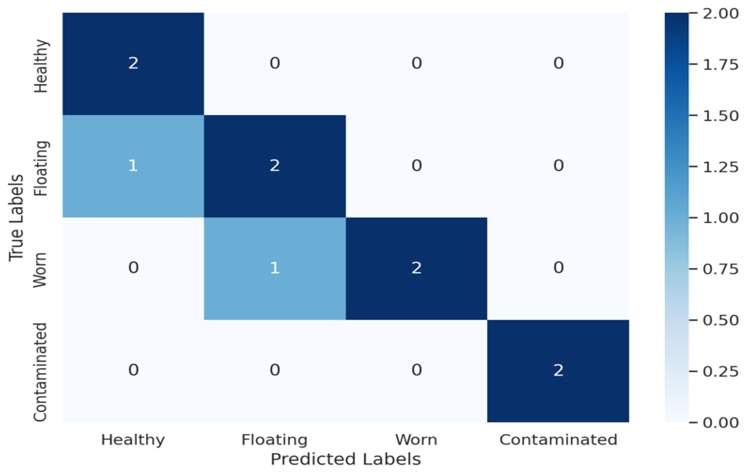
Figure 20 presents the confusion matrix, illustrating the model’s classification performance across all four brush conditions: healthy, floating, worn, and oil/dust contaminated. The matrix is predominantly diagonal, indicating high classification accuracy and strong fault class separability. Only two misclassifications are observed:

• One instance of a floating brush fault was incorrectly labeled as healthy;
• One worn brush fault was predicted as a floating brush fault.

These minor confusions likely reflect overlapping time–frequency patterns, such as intermittent conduction, fluctuating currents, and harmonic distortions. Importantly, contaminated brush faults were identified with 100% accuracy, and no healthy conditions were misclassified as faults crucial for avoiding false alarms.

These results confirm the CNN model’s capability to detect subtle spectral differences and distinguish diagnostically challenging brush fault scenarios, marking a significant improvement over threshold-based or manual diagnostic approaches.

These distinctions are subtle and often indistinguishable via manual inspection or threshold-based monitoring. The CNN’s ability to learn and discriminate these nuanced spectral–temporal patterns underscores the robustness of the proposed diagnostic framework.

In summary, the results confirm that the deep learning model not only reliably identifies healthy versus faulty conditions but also discerns between varying fault types with high precision. The model’s high sensitivity to early-stage degradation supports proactive maintenance strategies, while its accuracy in detecting severe faults enhances operational safety. These findings represent a marked advancement over conventional diagnostic methods, offering scalable and interpretable insights for real-time turbine generator monitoring.

6. Model Interpretability and Feature Attribution

To enhance the interpretability of the CNN-based fault diagnosis model and address its “black-box” nature, dimensionality reduction techniques such as t-distributed Stochastic Neighbor Embedding (t-SNE) and Uniform Manifold Approximation and Projection (UMAP) were employed. These techniques enable the visualization of high-dimensional feature spaces in two dimensions, offering intuitive insights into how the CNN internally organizes learned representations to distinguish between shaft earthing brush fault types.

6.1. Rationale for Using Multivariate Visualization

The rationale behind applying multivariate visualization techniques lies in their ability to transform complex, high-dimensional representations learned by deep networks. For fault diagnosis tasks involving subtle spectral variations, such visualization is crucial for

• Revealing latent structure in the learned feature space;
• Validating class separability, particularly when fault conditions exhibit overlapping or nonlinear characteristics;
• Providing transparency into how the model clusters similar fault conditions and separates distinct ones.

These visualizations serve as a bridge between model performance and domain-level understanding, offering stakeholders a tangible view of how fault-specific features are encoded. Such visualizations help build practitioner trust by providing tangible evidence of the model’s diagnostic logic and fault-specific sensitivity.

6.2. Selection of the Penultimate Layer for Visualization

Feature vectors were extracted from the penultimate (decision) layer of the trained CNN. This layer is typically responsible for encoding the most abstract and class-discriminative information before final classification. Unlike lower layers that capture more general or spatial features, the penultimate layer focuses on condensed, high-level representations that directly influence the output decision.

By visualizing the output of this layer, the analysis captures the final feature space used by the model to make decisions, allowing for the direct assessment of how well the model separates the various fault classes in its internal representation.

6.3. Importance of Dimensionality Reduction in Validating Learned Separability

The application of t-SNE and UMAP to the penultimate layer outputs provides complementary perspectives:

• t-SNE emphasizes local structure and preserves distances between nearby points, making it effective for identifying tight clusters of similar fault signatures;
• UMAP focuses on preserving both local and global data structure, offering a broader view of class relationships and inter-cluster boundaries.

6.4. Multivariate Visualization of Penultimate CNN Layer

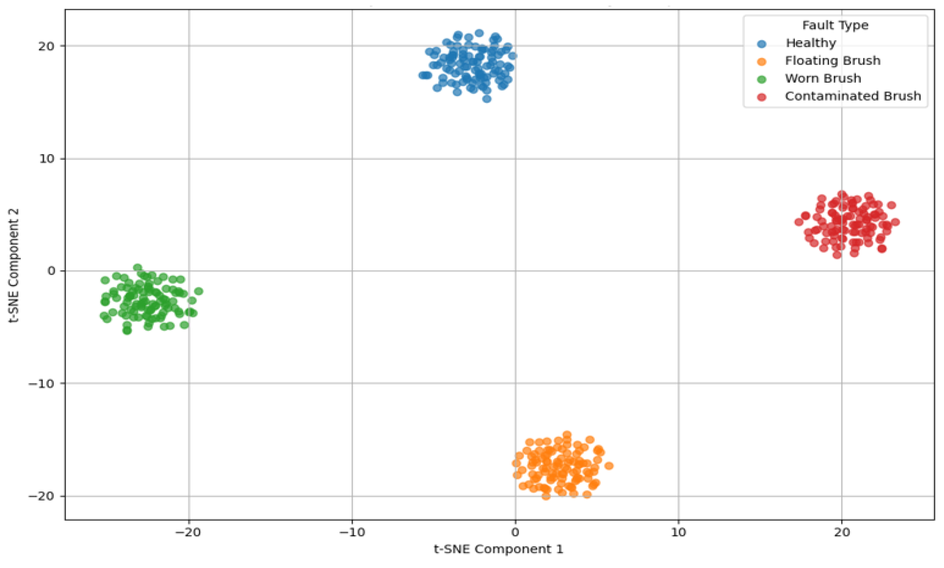
Figure 21 and Figure 22 display the t-SNE and UMAP projections of the CNN’s decision-layer feature embeddings. Each fault class forms a distinguishable grouping, indicating the successful encoding of class-specific spectral features.

This plot in Figure 21 shows the clustering behavior of features extracted from the final convolutional layer. Different fault types, such as healthy, floating brush, worn brush, and contaminated brush, exhibit partial separability. While some overlap exists, the clear grouping of “floating” and “contaminated” classes suggests that the CNN captures meaningful discriminatory features.

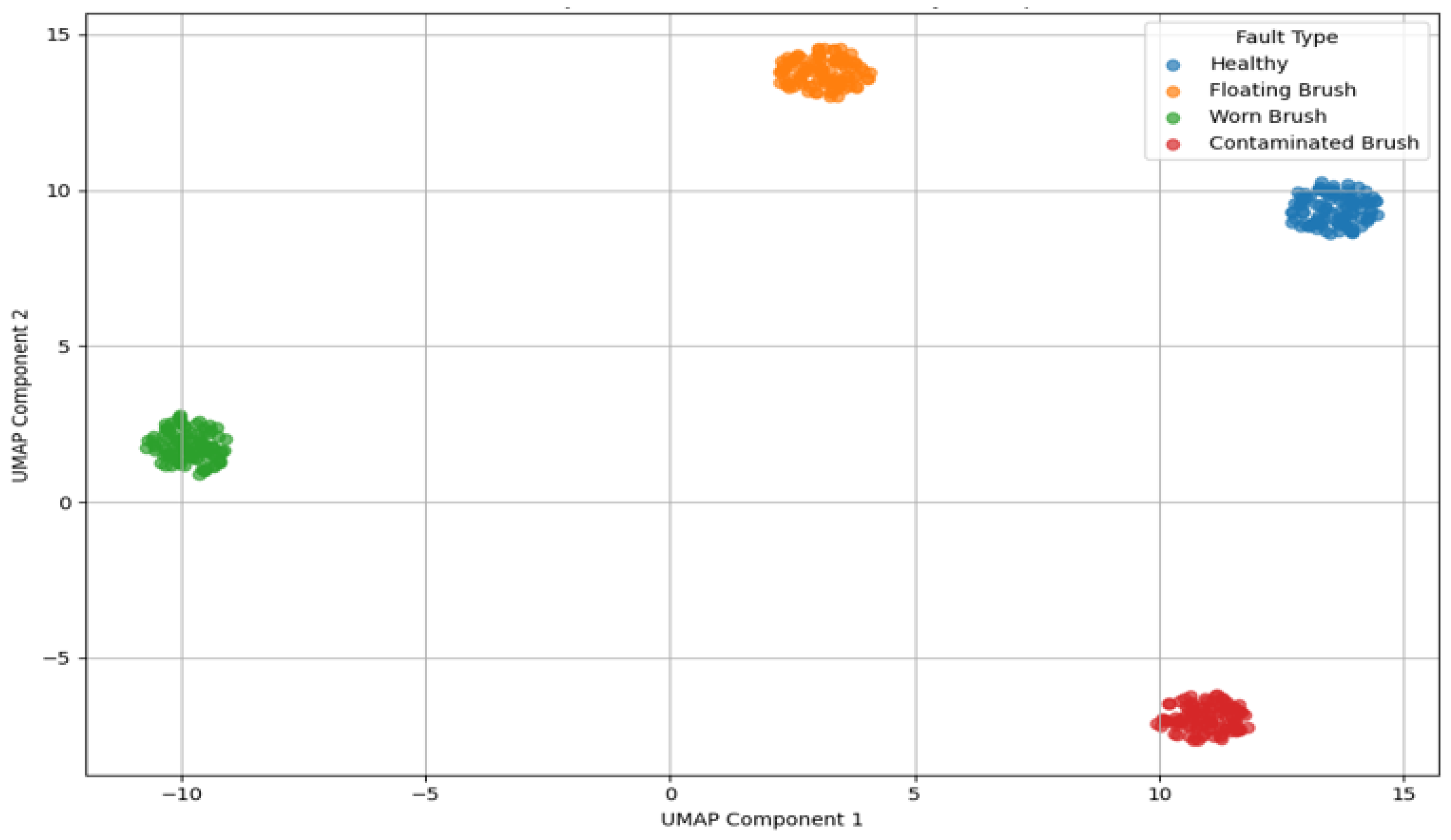
The UMAP in Figure 22 provides a more global view of data structure and corroborates the separability seen in t-SNE. The spread of data clusters further demonstrates that the CNN model captures subtle patterns linked to each fault type. These visualizations serve dual purposes:

• Validation of the CNN’s internal structure and class separability.
• Explainability, by converting abstract model representations into interpretable formats that support engineering insight.

The resulting plots (Figure 21 and Figure 22) reveal well-defined clusters corresponding to the four shaft earthing brush fault types: healthy, floating brush, worn brush, and contaminated brush. This visual evidence supports the model’s ability to learn fault-specific patterns that are statistically separable, reinforcing its diagnostic reliability and generalization capability. These findings substantiate the model’s transparency and enhance confidence in its deployment for practical fault detection in shaft earthing brush systems.

In summary, the integration of t-SNE and UMAP into the model assessment framework significantly strengthens the interpretability of the CNN model. This contributes to greater practitioner confidence and aligns with the best practices in explainable models for power system diagnostics.

7. Comparison with Conventional Methods

To put the performance of our deep learning-based framework into perspective, we compared it against conventional fault detection methods commonly used in industry for shaft grounding systems. Two such methods were evaluated: a simple threshold-based alarm on shaft voltage and a classical machine learning approach using manual feature extraction and a standard classifier (support vector machine (SVM)). The comparison highlights the advantages of the CNN approach in terms of accuracy, adaptability, and early detection capability.

In many existing generator monitoring setups, an alarm is triggered if the shaft voltage exceeds a predetermined threshold value for a certain duration. For our dataset, we determined a reasonable threshold by analyzing healthy data (virtually 0 V) and faulty data. A threshold of 5 V was chosen as a compromise, being higher than any healthy fluctuation but low enough to catch significant faults. We then applied this rule to the test data. The threshold method successfully caught all the complete brush failure cases (since those had voltages rising well above 5 V). However, it failed to detect the majority of the “brush wear” instances, because in many of those segments the voltage spikes, though frequent, peaked at only 2–4 V, below the threshold. By the time the brush wear fault progressed to generate >5 V spikes, substantial damage could have already occurred. Additionally, the threshold method exhibited occasional false alarms: a few transient events (likely high-frequency noise spikes) in the healthy data momentarily exceeded 5 V (when high-frequency components are not filtered, a short spike can have a high instantaneous amplitude). These false triggers would need further filtering in practice. Overall, the threshold-based scheme yielded roughly 70% detection of degraded brush faults and about 95% detection of severe faults, with a handful of false alarms, significantly inferior to the CNN’s performance of ~98% detection, with essentially no false alarms for healthy periods.

For a fair comparison with a more advanced baseline, we implemented an SVM classifier using several handcrafted features. These features included mean and standard deviation of shaft voltage, maximum voltage in the segment, frequency-domain energy in various bands, and the count of high-frequency spikes (detected via thresholding the derivative of the signal). We trained the SVM on the same training data that was used for the CNN. With careful feature selection and parameter tuning, the SVM achieved a respectable accuracy of around 90% on the test set. It performed well in distinguishing completely healthy vs. completely faulty states (similar to threshold method for obvious cases) but struggled with the intermediate “brush wear” class. Many partial fault segments were misclassified as normal or confused with full faults, as the handcrafted features could not always capture the subtle differences. In contrast, the CNN with its learned features handled these nuances much better. Another drawback of the SVM approach was the labor involved in finding good features and thresholds; the deep learning model automated that process. The deep learning framework clearly outperforms conventional methods on all fronts:

• The CNN’s ~98% overall accuracy beats the ~90% of the tuned SVM and far exceeds the threshold method’s performance. Particularly for early-stage faults, the CNN has a distinct advantage.
• Because the CNN picks up on patterns (frequency bursts, etc.) that occur before amplitude thresholds are crossed, it can alert for maintenance sooner. This could translate to addressing brush wear when it is minor, as opposed to waiting until it becomes severe enough to create large voltage excursions.
• The threshold method is rigid (one must set a fixed voltage limit). The CNN, however, effectively learned a multi-dimensional decision boundary in the feature space. It is more adaptable if the data distribution changes slightly; for example, if a new type of fault or a different generator introduces new signal characteristics, the CNN can potentially be retrained or fine-tuned, whereas designing new thresholds or features would require manual re-engineering.
• In our tests, the CNN had virtually no false alarms on normal data, whereas the simplistic threshold occasionally did. This is important for deployment, as frequent false alarms can lead operators to distrust or ignore the monitoring system.

It is worth noting that the conventional methods are simpler and require less computational power, which historically made them attractive. However, with modern processors and the relatively small scale of our CNN, real-time computation is quite feasible. The CNN processed data in real-time during our experiments with ample margin (each inference taking only a few milliseconds on a standard CPU, which is well within the time of incoming new data segments). Therefore, the computational overhead of the deep learning approach is not a limiting factor in practice.

In conclusion, the comparison strongly favors the deep learning diagnostic framework over traditional methods for the task of earthing brush fault detection. The high inaccuracy and responsiveness justify the use of the CNN approach, especially in critical systems like power generators where the cost of failure is high. Next, we discuss the broader implications of these findings and how this approach fits into the landscape of predictive maintenance for electrical machines. Furthermore, the threshold-based approach cannot classify the type of fault; it can only issue a generic warning that “something is wrong”. In contrast, this CNN model provides detailed information on the fault category, which can help maintenance personnel identify the root cause more quickly. This comparison underscores the benefit of the proposed intelligent diagnostic system: it offers both higher sensitivity and richer diagnostic insight than conventional monitoring techniques.

8. Key Findings and Discussion

The performance of the deep learning diagnostic framework was evaluated using the experimental dataset collected from a fleet of large-scale turbine generators. The fault signatures presented were obtained through a combination of site-based experimental testing and historical data collection from multiple power stations operating hydrogen-cooled generators ranging from 200 MW to 846 MW at 22 kV. The framework’s ability to detect faults and distinguish between fault types was assessed in terms of classification accuracy, confusion matrix analysis, and comparison with traditional monitoring metrics.

The strong performance of the deep learning framework can be attributed to several factors. First, the use of time–frequency features proved crucial. Our preliminary tests showed that the CNN performed better with spectrogram inputs than when trained directly on raw time-series data. The time–frequency transformation acts as an implicit feature extractor, emphasizing fault-related characteristics (like transient bursts or spectral content changes) that the CNN can easily learn. This finding aligns with observations from other studies that applying time–frequency analysis can enhance fault detection in non-stationary signals [11,12].

Second, the CNN’s architecture, though relatively simple, was sufficient to capture the complexity of the patterns in the data without overfitting. By using a moderate number of filters and layers, along with data augmentation and early stopping, we ensured that the model generalized well to new data. The confusion matrix and nearly perfect classification metrics on the test set suggest minimal overfitting. We also conducted a cross-validation by training the model multiple times with different random weight initializations and data splits; the performance varied only slightly (±1–2%), indicating the model is stable and the results are reproducible.

The results of this study demonstrate that a deep learning-based approach can significantly enhance the monitoring of shaft earthing brushes in large generators. Below we highlight the key findings and discuss their implications for both the research community and industry practitioners:

• The CNN-based framework detected subtle brush degradation patterns that conventional threshold methods overlooked. For instance, intermittent contact losses producing only small voltage spikes were reliably identified. This early detection capability is crucial because it provides maintenance personnel with advance warning to address brush wear before it escalates into a serious fault. By catching issues at an incipient stage, operators can schedule timely maintenance (such as brush replacement or cleaning), thereby avoiding unexpected generator trips or bearing damage.
• The diagnostic system achieved near-perfect accuracy on the test data, with >98% correct classification overall. In practical terms, this means the system is highly reliable and that it almost never misses a true fault and rarely issues a false alarm. Such performance is essential for building trust in automated monitoring. Plant operators can be confident that when the system flags a brush issue, it is very likely legitimate. Conversely, if the system reports healthy operation, the probability of an undetected fault is extremely low. This level of reliability approaches that of human expert inspection, if not exceeding it, especially since the system can monitor continuously without fatigue.
• The framework proved robust to variations in operating conditions (like generator speed and excitation levels). It indicates that the learned features are generalized representations of the fault conditions, not just memorizing specifics of one operating point. This is encouraging for real-world deployment, where conditions fluctuate and a model must tolerate some variation. The use of normalization and time–frequency features, as well as training data covering different scenarios, contributed to this robustness.
• Our comparative analysis showed that traditional monitoring could miss up to 30% of early-stage faults and produce false alarms, whereas the CNN approach dramatically reduces those shortcomings. This underscores the value of applying modern AI techniques to long-standing industrial problems. It aligns with broader trends in predictive maintenance: machine learning is increasingly being adopted to replace or augment simpler threshold-based systems, yielding better predictive power and insight.
• Although this work focused on shaft grounding brush faults, the successful demonstration of the approach suggests that it could be extended to other related problems. Large turbine generators have many components (bearings, windings, etc.) whose incipient failures might also be detectable through subtle changes in electrical or vibrational signals. The methodology of combining domain-specific signal processing with CNN-based classification can be a template for designing diagnostic tools for those subsystems as well. Additionally, this research contributes to the growing field of digital twins and smart diagnostics in power generation, where data-driven models continuously assess equipment health and predict failures before they happen.

While the findings are highly positive, we also acknowledge some limitations and future directions:

• The model currently treats the problem as a classification among discrete states (normal, wear, failure). In reality, brush degradation is a gradual process. A potential improvement would be to formulate the problem in a regression or remaining useful life (RUL) estimation framework, wherein the model could output a health index or an estimate of how much life is left in the brush. That would directly support maintenance scheduling.
• Interpretability of deep learning models is an ongoing challenge. While we trust the CNN’s outputs due to its high performance, understanding which features in the signal it bases its decisions on can further increase confidence. Techniques such as saliency maps or explainable AI methods could be applied to highlight portions of the waveform or spectrogram that the CNN finds indicative of faults. This could provide engineers with physical insight (e.g., confirming that the model looks at high-frequency bursts for arc events, etc.) and help troubleshoot any odd predictions.

Overall, our deep learning-based approach is highly effective for SEB fault diagnosis and holds promise for real-world deployment. It provides a clear improvement in fault detection capability over traditional methods, which can significantly enhance predictive maintenance strategies for large generators. By enabling the early and accurate detection of brush deterioration, this framework can help prevent serious damage to generator components and reduce maintenance costs. These findings reinforce the potential of deep learning-based diagnostics as a transformative tool in generator maintenance practices that is capable of shifting from reactive to predictive maintenance frameworks.

Although the proposed fault classification framework was developed and validated under controlled testing conditions, it is designed with real-world deployment in mind. The data used for training and evaluation were collected from operational turbine generators during both healthy and induced fault scenarios, ensuring practical relevance. However, field deployment may introduce additional challenges such as ambient electrical noise, variability in generator architectures (e.g., hydrogen-cooled vs. air-cooled units, different excitation systems), and differences in shaft grounding brush configurations. These variations can affect the input signal characteristics and model inference accuracy. To address these uncertainties, the model training process incorporated data augmentation techniques such as random intensity scaling and the time shifting of spectrograms to simulate the kinds of signal fluctuations that may occur during normal plant operations. Furthermore, future work will focus on integrating the trained model into utility’s existing online monitoring systems to assess its performance under live operating conditions. This real-time validation phase will include feedback from plant personnel and comparison against conventional threshold-based diagnostics. To enhance adaptability, techniques such as domain adaptation and incremental learning will be explored, allowing the model to fine-tune itself based on generator-specific characteristics. These steps are critical for ensuring robust performance and scalability across the utility generation fleet.

In conclusion, the discussion affirms that the deep learning diagnostic framework not only achieves excellent technical results for shaft brush fault detection but also fits well within the practical requirements of generator maintenance. By improving early fault detection and reducing false alarms, it can contribute significantly to more reliable and efficient power generation operations. The next section provides a brief conclusion of the study and outlines key takeaways.

9. Conclusions

This study presented a deep learning-based diagnostic framework for detecting shaft earthing brush (SEB) faults in large turbine generators. Recognizing the importance of shaft grounding in mitigating destructive voltages and bearing currents, we proposed a methodology that combines frequency-domain signal processing with a convolutional neural network (CNN) classifier to automatically identify brush degradation conditions. The framework leverages Fast Fourier Transform (FFT)-derived spectrograms of shaft voltage and current signals to enable the multi-class classification of fault types, including floating contacts, worn brushes, and contamination.

Experimental evaluations on both real-world and simulated fault conditions demonstrated the model’s high diagnostic accuracy, achieving approximately 98% classification performance across four fault categories. This significantly outperforms conventional threshold-based monitoring, particularly in identifying early-stage or subtle brush degradation. By encoding time–frequency features into grayscale spectrograms, the CNN was able to learn complex fault patterns that are difficult to capture with manual feature extraction. Key findings include the following:

• FFT-based spectrograms of shaft voltage and current effectively encode diagnostic features for brush fault detection.
• Dual-channel CNN input improves fault-type discrimination by jointly analyzing voltage and current domains.
• The model demonstrated high sensitivity and specificity in classifying different SEB fault conditions.
• Data augmentation and stratified splitting improved generalization, reducing overfitting risks on limited data.

Despite its success, the study has limitations; one of the primary limitations of this study lies in the imbalance and scarcity of certain fault conditions in the available dataset, particularly for rare failure modes such as oil/dust contamination or floating brush faults. While the CNN-based model performed robustly on the available real-world data, its generalization could be further improved with more diverse and representative training samples. To address this, future work will explore the use of Generative Adversarial Networks (GANs) to synthetically augment the dataset. GANs have shown promise in generating realistic time-series signals and spectrogram representations for fault diagnosis tasks in other domains. By training a GAN to simulate fault-specific signal patterns, especially for underrepresented classes, we aim to enhance model robustness, reduce overfitting, and enable more balanced classification performance. This approach aligns with recent advances in data-driven reliability modeling and offers an opportunity to scale fault diagnostics across broader industrial applications.

Future work will also focus on deploying the framework in live generator environments. This includes integrating with real-time monitoring systems, expanding to different generator types and excitation systems, and applying adaptive learning techniques like transfer learning or incremental updates. Further enhancements may include estimating fault severity or predicting remaining useful life (RUL), transforming fault detection into a predictive maintenance tool.

In conclusion, the proposed CNN-based diagnostic system marks a significant advancement in the condition monitoring of rotating electrical machines. By automating fault detection through learned time–frequency representations, it offers a scalable, accurate, and practical solution for the early detection of SEB faults. This contributes to improved reliability, reduced downtime, and optimized maintenance in power generation facilities.