Abstract
Wind farm performance monitoring has traditionally relied on deterministic models, such as power curves or machine learning approaches, which often fail to account for farm-wide behavior and the uncertainty quantification necessary for the reliable detection of underperformance. To overcome these limitations, we propose a probabilistic methodology for turbine-level active power prediction and uncertainty estimation using high-frequency SCADA data and farm-wide autoregressive information. The method leverages a Stochastic Variational Gaussian Process with a Linear Model of Coregionalization, incorporating physical models like manufacturer power curves as mean functions and enabling flexible modeling of active power and its associated variance. The approach was validated on a wind farm in the Belgian North Sea comprising over 40 turbines, using only 15 days of data for training. The results demonstrate that the proposed method improves predictive accuracy over the manufacturer’s power curve, achieving a reduction in error measurements of around 1%. Improvements of around 5% were seen in dominant wind directions (200°–300°) using 2 and 3 Latent GPs, with similar improvements observed on the test set. The model also successfully reconstructs wake effects, with Energy Ratio estimates closely matching SCADA-derived values, and provides meaningful uncertainty estimates and posterior turbine correlations. These results demonstrate that the methodology enables interpretable, data-efficient, and uncertainty-aware turbine-level power predictions, suitable for advanced wind farm monitoring and control applications, enabling a more sensitive underperformance detection.
1. Introduction
Wind is a renewable energy source that has become more important in recent years; therefore, wind farms have been deployed around the globe to generate electricity. This growth follows the need and search for alternative energy sources to decarbonize power grids to reduce pollution. To extend wind energy as profitable, the Levelized Cost of Energy needs to be further reduced. Due to this, challenges related to advanced performance monitoring need to be solved to accurately assess the possible power production and be able to quantify the energy losses created by certain O&M decisions [1]. Nonetheless, it is not straightforward to estimate possible power and the normal behavior of the production during wind conditions measured by anemometers when using high-resolution data [2].
SCADA systems are, in the majority, capable of capturing data at high frequencies such as 1 Hz. However, in most cases, the data is resampled to 10 min for analysis, losing certain physical properties of the data. As stated in [3], this low frequency can negatively impact Condition Monitoring capabilities.
Initially, research related to active power production has focused on using power curves either by engineering models [4,5,6] or more data-driven models [7,8]. The methodologies mentioned here are mostly based on resamples of 10-minute data. Machine learning techniques that are less related to power curve modeling have also been researched to output active power predictions both on high frequency [9,10,11,12] and lower frequency [13,14]. However, as mentioned earlier, they still focus on predictive power and do not examine the variability. Having an estimation of variability permits understanding of the normal behavior in a turbine.
Uncertainty estimations under normal conditions have not been thoroughly studied [9] or have been based on Gaussian assumptions around the power curve. The thresholding that measures the uncertainty of the production is necessary to study, given that the performance has significant variations under normal operating conditions and similar atmospheric conditions [15,16]. This highlights certain disadvantages of conventional power curves. Including lagged inputs as part of the model is supposed to provide a better estimation of the variance and covariance inside the wind park. These approaches provide an initial individual turbine approach, which ignores the fact that in wind parks, turbines have covariances by not taking into account the model’s farm-wide data. The inclusion of data from similar turbines is useful to provide a better variability estimation.
Further approaches like those in [10,11,12,17] based on high-frequency data have been focused on more accurate predictions. Nonetheless, they keep providing a deterministic predicted value instead of credible intervals, where we could expect the real value of active power. Models that have a more informed conditional variability could give more accurate uncertainty estimations, therefore providing a better interval of proper behavior. The model presented here might sacrifice some accuracy to provide a white box prediction, which is not only traceable but also interpretable based on simple concepts such as correlation. These correlations are expected to be informed by both farm-wide and auto-regressive components. In spite of their results in predicting and profiting from the use of farm-wide data, these approaches are missing a proper study of the analytical variability that is inherent in the system.
Developments in the computation of Gaussian Processes permit taking inference, in general, for any function, as established by [18,19]. This opens the possibility not only to use machine learning or statistical functions but also to use inference on physical functions. Here, when inference is mentioned, it is with the understanding of Statistical Inference, which is particularly interested in allocating variability and a probability distribution. In this, Gaussian Process Regression provides a powerful framework for using any function as the mean function [18,20], allowing a point prediction with prior knowledge. These developments permit the use of functions, such as the power curve, as prior knowledge in an inferential system with further use in Multi-Task modeling for compiling farm-wide information.
The rationale for these high-frequency predictors lies in the ideas of [21] of a “micro-prediction oracle”. The oracle, as defined in the aforementioned, is an imperfect but powerful tool that is as accurate as possible. It is possible to advocate that the power curve is an oracle, and the work here is adding a data-driven correction on top of an uncertainty estimation. Knowingly, this can be extended to other prediction methods, as discussed in [20]; nonetheless, this will be discussed more thoroughly in further work. Given the initial simplicity, it is easy to produce methods that use the information of the power curve in their estimations.
The relevance of having estimations and uncertainty is important because it provides an analytical approach to understanding underperformance. Based on these two values, it is possible to infer probabilities of underperformance by making Gaussian assumptions. This will permit inferring underperformance by the constant check of their probabilities. If possible, and with further tuning, this also opens the possibility of inferring more rigorously with a more appropriate distribution. This changes the approaches used commonly in the literature from a deterministic way of seeing power production to a more stochastic one, opening the possibility of calculating losses of energy on a certain interval.
The main takeaways from the existing work are that there are methods to estimate active power accurately on a farm-wide level, and there are methods to assess the variability of the normal behavior of a turbine. There is a methodological need to have both together, given that including estimations of the variance and correlations helps the modeling of joint uncertainties. This can provide information about underperformance and can provide information to other algorithms about the expected behavior. The methodology presented here is designed to put together the active power estimation methods and the variability estimation for normal behavior.
The proposed work has the objective of providing predictions and uncertainty estimations of active power using all the possible wind farm information. Specifically, it is expected to propose a statistical methodology for expected active power prediction and its uncertainty, preferably one that can be explained with simple statistical properties. This methodology intends to leverage both farm-wide and auto-regressive information, even if it is implicit, profiting from information of the signal. Lastly, the methodology should be flexible and work independently of how the prediction of the active power is structured.
The idea is to provide an initial glimpse of methodologies that include variability as part of the modeling framework. From the methodology presented here, the methods and the mindset can be transferred to other methodological approaches. The mindset looks to establish a combination of physics, machine learning, and probabilistic approaches.
In the following sections, the methodology will be presented in detail. Based on this, results will be presented afterward, followed by an extensive discussion and conclusions. The purpose is to show, based on a previous study, a methodology to solve the uncertainty of power production estimations under normal operating conditions using data-driven methods.
2. Methodology and Modeling Approach
The study aims to provide a model that uses farm-wide information to exploit the autoregressive relationships that could exist in a wind farm. As mentioned in [11], one can profit from the use of Time Series Analysis to provide a proper methodological solution.
The methodology presented here will be based on Gaussian Process Regression (GPR). Specifically, GPR techniques related to Multi-Output modeling will be presented. To have theoretical clarity, from now on, when referring to as a task, it will refer to the active power produced. X will be the inputs from the whole farm, which could change according to what is being explored.
Just like in [11], the work here attempts to present a Time Series Analysis perspective. The latter is expected to also consider that implicitly physical relationships (wake effects) inside the wind farm are taken into consideration. This last point is tackled by including information from the lagged inputs of the data. Therefore, in a minimalist way, a functional way of representing this is as follows.
where represents the active power of a turbine. The inputs X inside the function might vary according to how we define the mean function inputs. It is, overall, expected to include information from the wind speed, past wind speeds, the wind direction, and the past wind direction.
The study also addresses the fact that the distribution of the active power in a wind farm has variations even under normal operating conditions and the same environmental conditions, as mentioned in [9] based on the work presented in [15,16,22].
Furthermore, the work presented here focuses on having both a prediction and an uncertainty estimation. The idea is that this uncertainty estimation can also be done independently of the function that describes the expected value of the wind power production.
2.1. Data
The data presented here comes from the SCADA system of a Wind Farm present in the North Sea of Belgium. This park has more than 40 turbines. The SCADA data is annotated with curtailments, transients, and alarms on a 1 Hz frequency. This is based on the methodology presented in [23]. The annotations will be discussed, and the data cleaning was based on that. From this, it was resampled to a 10 s frequency. This addresses certain dimensionality problems without particularly sacrificing the signals’ properties.
To show the data efficiency of the method, the training set constitutes a very small part of the available dataset. This constitutes the data points from the first 15 days of year 1. The rest of the dataset from year 1 was used as validation, and the entirety of year 2 was used as a test set. It is important to note that these years are adjoining each other.
2.1.1. Data Annotation
Based on the aforementioned work, the curtailment methodology used a subset of machines to detect underperformance across the fleet, and they were combined with status logs. The transients were based on start-ups and coast-downs, and they were manually annotated based on data conditions; this was done with an expert identifying them inside the short label dataset. Finally, the alarms were based on a multi-step processing scheme that comes from raw vibrations and automated alarm indicators. The methodology follows exactly what is described in [23,24].
The annotation of the curtailments is constituted when several turbines produce less than their expected power curve value. These events are known to the controller, and in general, several turbines are reduced to an equal amount, which permits easy recognition. Therefore, this annotation is based on the annotations from the controller and the behavior of the turbine as an ensemble.
For the cases of transients, this annotation is based on status logs from the turbines. This process is done manually on the data, and it is dependent on the controller, given that the controller has different braking and start-up programs at display.
Finally, the alarms were also annotated manually based on the status-logs from each turbine. The information comes from both the acquisition system and information provided by the controller. After that, based on the aforementioned, the dataset was annotated.
2.1.2. Data Filtering/Outlier Removal
To have data for the expected, or normal, behavior, any faulty farm-wide observations were not taken into account. This means that anomalous observations were filtered out of the dataset. The faulty observations were considered as the annotated transient, curtailments, and alarms that were mentioned beforehand.
On top of those faulty observations, SCADA observations with 0 or negative active powers were excluded. This is important given that some of these observations were not annotated into the transients, alarm, or curtailments. The amount of observations can be seen in Table 1.

Table 1.
Data points included and excluded.
Apart from excluding these observations, there was no other type of filtering or outlier removal. Anything outside of these situations was considered normal behavior of a turbine.
2.1.3. Scaling of the Data
Throughout the work presented here, the data used to both fit and predict the model was rescaled using Min–Max rescaling. For the specific case of the wind direction, these channels were handled using their and to not lose distributional properties, as discussed in [25], it is one of the best approaches for circular data.
The re-scaling, therefore, was performed as follows
These maximum and minimum values were not thought of in a data-driven manner. This max was based on theoretical values, based on the rated speed. This scaling has the rationale of keeping numerical stability. Thus, the output (active power) min is 0, and the max constitutes rated power. The min wind speed was also set to 0, and the max wind speed was set to the wind speed at the rated power. In machine learning, this is a common practice for the normalization of data.
This scaling is preferred because it keeps the distribution of the features between 0 and 1, preventing it from having large magnitudes that disproportionately affect relationships between the input and output. This method also preserved the original shape of the distribution and helps with numerical stability.
2.2. Intrinsic Model of Co-Regionalization (IMC)
Initially, as described in [26,27], this approach bases itself on having a set of X distinct inputs of size D and a set of M outputs. Therefore, this is thought to be a problem . Under this particular framework, it is thought that the data structure goes as .
As described in [11], based on the works of [28], the model presented there consists of
This particular model, which was described in [11], has a data structure where . M represents the turbines. Therefore, to include farm-wide information, each task would need to have the same information, which makes the model quite computationally complex. This model, as it was described, has the particularity of permitting conditional independence when predicting.
While the data structure can be adjusted to use farm-wide information, doing so is computationally expensive. Therefore, a priori, it was concluded that a less computationally expensive method that uses farm-wide information can be used. This is because, based on this model, one would have M equations that include information about the whole system.
2.3. A Model Using the Whole System
As discussed in the last section, the IMC will produce results where the mappings are completed as , which could over-look inter-domain dependencies between tasks, specifically for the case of turbines. The model that is proposed here permits inter-domain mean functions and variability estimations. Here, it is intended to use a lower-dimensional space that is referred to as L in [27], which will represent the independent functions .
If it is pursued to achieve a model that takes into account inter-domain variables, it is necessary to use a different approach. This approach can be provided with a Stochastic Variational Gaussian Process Regression (SVGP) using as a prior the Linear model of Coregionalization (LMC), as described in [27]. The approach mentioned here will consider a regression problem of the form . In this case, D will represent the dimensional space of the inputs, which could vary according to the information available. It is intended with this to build a data structure of the more generalized way , where i represents the index of the task, and X includes information associated with all the tasks. Therefore, as explained in [27], we have the assumption of a model of the form.
where the outputs are assumed to be independent and, by mixing them with the W matrix, they become correlated. It is important to highlight that the W matrix needs to be . This permits having a shared Kernel for the whole system and being capable of estimating each , therefore, enabling the use of farm-wide information to provide predictions. The function for can be manipulated and estimated, as mentioned in [20]; further in the work, this will be discussed more thoroughly. As mentioned in [27], this brings the implication of a covariance in the following way.
where L is a lower-dimensional explanation; therefore, it is implied that , where L represents the Latent Gaussian Processes involved. Even though theoretically, L can be of dimension 1, it is suggested to use a higher-dimensional space, given the fact that if only one latent space is used, the covariance between the turbines will be perfect in the posterior distribution. It is also necessary to highlight that when , the system is assumed to be independent. The number of Latent Gaussian Processes explored is 2, 3, 5, 8, and 10; further latent spaces have very high memory requirements even when using stochastic optimizers.
In the end, from the theoretical background given, it can be inferred that ; therefore, distributionally looking as
The SVGP profits from the use of Stochastic Variational Inference, which, as defined in [29], is an attempt to approximate a conditional density of latent variables given the observed variables. This is done using the Kullback–Leibler divergence to the exact posterior, which constitutes a statistical distance. For information purposes, the formula will be presented here
From there, it is thought to change the inference problem into an optimization problem. Taking the conditional as suggested in [29], concerning , one has the following conditional, which is dependent on
Nonetheless, the KL divergence cannot be computed; therefore, leaving the need to optimize an alternative objective function. This alternative is called the Evidence Lower Bound (ELBO), which is an alternative to KL with an added constant. The ELBO will represent the loss function of the optimization process of the SVGP. The ELBO has the following formulation
The premise behind using this, as formulated by [29], is to transform an inference problem into an optimization problem. In the end, as mentioned in [19], one of the big advances suggested in the work provided in [30] explicitly keeps the structure of inducing variables.
Based on experimental results, it is necessary to take into account certain practical implications. It is important to consider that the batch size is recommended to be higher than the number of columns in the input matrices.
2.4. Choice of Kernel
To model the behavior of the covariance function, the Matérn Kernel was used. This is due to its studied generalization power. The Matérn Kernel has the parameter and for the model usage, this parameter will be set to . This is because, according to [18], based on the work in [31,32], this shows one of the most important results. Therefore, can be expressed as
2.5. Meta-Modeling and the Mean Function
The following study is intended to show the flexibility of the presented methodology; therefore, as discussed in [20], several mean functions can be utilized under this methodology. For the specific proof of concept, the power curve will be the model presented here. Given that the power curve constitutes a physical law of wind that, according to [33], citing [34], follows the equation,
where represents the density, A the swept area, represents the wind speed at time t, and is the power coefficient. On how the mean function is thought here, only is not a constant. The values from this function, according to the wind speed, were provided by the manufacturer, so they are extracted from that data. The inferential framework presented here enforces the final outputs, , to be correlated as part of the posterior probability distribution.
The inputs between the mean function and the inferential system will differ for this specific case. This can be tweaked by using different mean functions, but it runs out of the scope of the work presented here. Therefore, the W matrix that is mentioned beforehand can function as a correction of the power curve that is informed by the last observed values of the system. This is given that the W matrix is included in the optimization of the inferential system, as part of the Coregionalization, which includes lagged information in the Kernels.
2.6. Hyper-Parameter and Parameter Tuning
As described in [18], there are sets of hyperparameters that are required by the Kernel functions that are left to vary; namely, the hyperparameter ℓ presented in the Kernels section needs to be optimized. There are several ways to optimize these hyperparameters; nonetheless, based on the aforementioned literature, it is possible to do it via Bayesian methods. Hyperparameter optimization is normally performed by optimizing the Log Marginal Likelihood function or the ELBO that was mentioned above. Nonetheless, because the purpose is to use computationally simpler methods, as explained in [35] and mentioned before, this Log Marginal Likelihood function is an approximation based on the lower bound of the same function, which was described before.
As established by [29], the ELBO, which is our chosen loss function, generally poses a non-convex problem. Therefore, first-order methods without a lot of information can become stuck in local optimum points, leading to inaccurate conclusions. First-order optimization methods, such as Adam [36], rely on local gradient information. In complex loss functions, this can cause the optimizer to become stuck on a local optimum, which does not provide the best information.
To address this, it is usually suggested to use second-order methods, like LBFGS, as they include curvature information through approximations of the Hessian. Nonetheless, these methods are computationally very expensive and pose difficulties in batching, making them impractical for large-scale data combined with complex structures. Instead, it was decided to adopt a combination of two strategies to improve convergence: learning rate schedulers and natural gradients in each step. Learning rate schedulers ensure a better convergence, even when the loss surface is quite complex [37]. For the work presented here, the Cosine Annealing scheduler is used. The natural gradients are used according to what is explored in [38] for the Variational Parameters.
2.7. Model Validations
To compare and assess whether the model error metrics will be used to validate the proper modeling of steady behavior, the Mean Absolute Error (MAE) and Root Mean Squared Error were used, as well as Mean Absolute Percentage error.
To check the goodness of fit, the or coefficient of determination was assessed in the following way.
where and .
This measure is usually performed on training data. Nonetheless, in this case, they will be performed on training and validation, given that the mean function is technically pre-fitted already.
In addition, physical validations based on the wake are similar to the ones presented in [10,12], as defined in [12],
where represents the active power of a turbine at timestamp t, is the estimated active power of the freeflow at time t, and n is the number of turbines. This is performed to make sure the behavior of the wake is being properly modeled.
3. Results
The experiments presented here are based on 1 year of data. The results presented are for data resampled to 10 s. For the error measurements and measurements related to the wake coefficients, timesteps with non-steady behavior were filtered out. By non-steady, it is implied that the turbine was not operating under the expected proper behavior. In this section, the method proposed adds a vector of parameters to the already known power curve. Due to this, the manufacturer’s power curve is the benchmark, and when referred to as only power curve, it refers to the manufacturer-provided power curve. All of the analyses were compared to this power curve, which was provided by the manufacturer without uncertainty estimations.
3.1. Power Curve as a Mean Function
To demonstrate the impact that the method has to induce changes in the final prediction, the manufacturer’s power curves were used. Since this method uses the manufacturer’s power curve, the mean function input constitutes only the instantaneous wind speed for each turbine. Therefore, the inputs used for the Kernels and for the power curve differ. The inputs that go into the Kernel, and hence, the inferential system of the Gaussian Process, constitute the 15 past observations of wind speed and wind direction.
Nonetheless, in the final prediction, this should differ by the use of the W parameter presented in the Coregionalization model. For the Kernels, the input constitutes the data from 15 lags of the wind speeds for each turbine and the wind directions reported in each turbine. As can be seen on the validation set of all free-flow wind directions independent of the parameter L, the prediction tends to be more accurate than the manufacturer’s power curve (Figure 1).
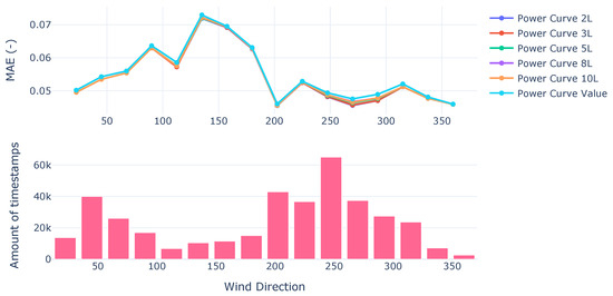
Figure 1.
MAE from power curves on validation set.
Initially, it is necessary to make sure that the model overall performs better than the power curve provided by the manufacturer (Table 2 and Table 3).

Table 2.
MAE, RMSE, , and MAPE calculated on the validation set.

Table 3.
MAE, RMSE, , and MAPE calculated on the test set.
The analysis of the results was performed based on the wind direction. This is to be able to assess all possible scenarios according to what we have available on the SCADA dataset about environmental conditions.
Similar behavior is seen on the test set (Figure 2); nonetheless, for wind directions that have a low amount of data, the use of any L does not improve predictions. This behavior can be seen in Figure 2.
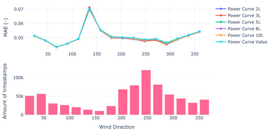
Figure 2.
MAE from power curves on test set.
Overall, the behavior is similar over the validation and test set. The improvement given by the inferential system can get up to on the MAE under dominant wind conditions. This happens when using a low amount of L, preferably between 2 and 3.
Similarly with the MSE, which constitutes , the aforementioned behavior is seen (Figure 3). The error measures seem to overall converge to the improvements given by the inferential system, which are marginal but yet present.
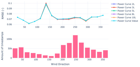
Figure 3.
RMSE from power curves on test set.
Among all error measurements, there is a consistent behavior where and perform worse than the power curve on free-flow wind directions with a low amount of data. The higher L is, the more robust under those wind directions with a low amount of data.
Overall, from , it can be seen that there is an improvement in the variability explanation (Figure 4 and Figure 5). The improvement oscillates at the same percentile gains discussed in the other error metrics. This can be attributed to the inclusion of the farm-wide covariance and the interaction with the lagged inputs.
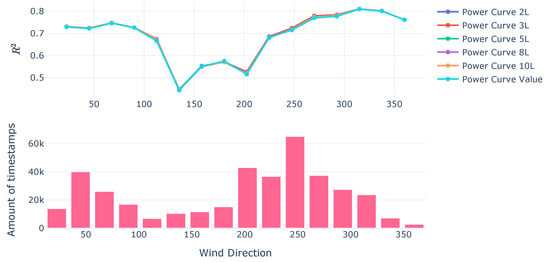
Figure 4.
Power Curves on Validation Set.
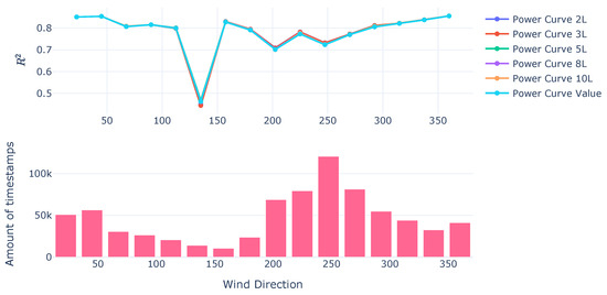
Figure 5.
Power curves on test set.
The MAPE converges to what has been seen in other error metrics (Figure 6 and Figure 7). Nonetheless because of the scale it looks less noticeable on visualization.
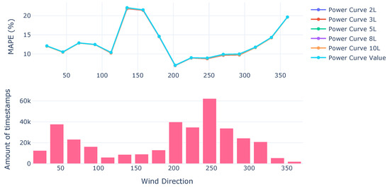
Figure 6.
MAPE power curves on validation set.
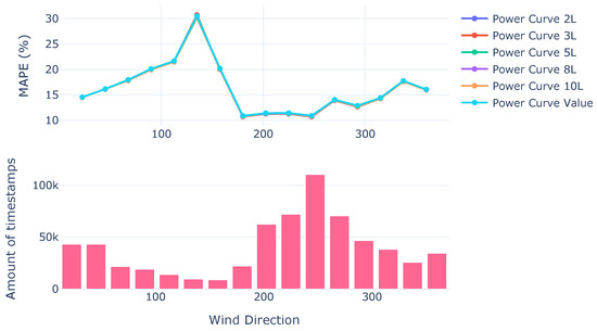
Figure 7.
MAPE power curves on test set.
As can be seen in the error metrics, the power curve provided by the manufacturer performs worse than the inferential system proposed—even if it is marginal. In the park-wide corrections, the difference can mainly be seen during dominant, or more common, wind directions. As can be seen overall, the proposed methodology improves the error measurement in between and for dominant wind directions. It is important to highlight that the difference is higher as there are fewer Latent GPs, denoted by the variable L.
Overall, this suggests that data availability plays a good role in the increased performance of any of the models. Under other environmental conditions, the gain of the model is not as noticeable, and it would rely on the variance estimations.
3.2. Validation of Wake Coefficients
As can be seen in Figure 8, the model replicates the Energy Ratios from the SCADA. This indicates that the model effectively captures the system’s underlying physics on the dominant wind directions, which are on the interval from 200 to 300. It can also be seen that as the accuracy of the model improves, the replication of the Energy Ratios from SCADA improves.
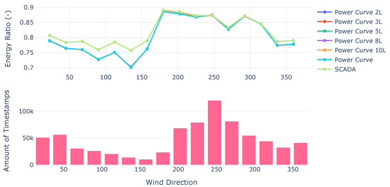
Figure 8.
Energy Ratios per model for the year 2021.
The models follow the trend of the power curve provided by the manufacturer, having very small changes in the dominant wind directions. Data availability has a big impact on how the models perform and how the power curve is corrected according to farm-wide lagged inputs.
One could speculate that either the values of the free flow are high or overestimated by the model when in non-dominant wind directions. Similarly, it could be attributed to the fact that waked turbines are being under-estimated. This happens mostly in non-dominant wind directions, which could be related to the bias of the power curve to not include any pitch misalignment.
Despite the fact that here, only the MAE is presented, the RMSE is added in the Appendix. Changing the error measurement does not have a great impact, given that the results on both converge. Therefore, it will converge to similar conclusions.
3.3. Uncertainty Estimations
The uncertainty measures should change according to the input parameters. This means that, according to the wind’s direction and speed, the active power’s variance should move accordingly, as seen in Figure 9. The one with the highest magnitude in the variance tends to be the one with the highest L, as shown in Figure 9.
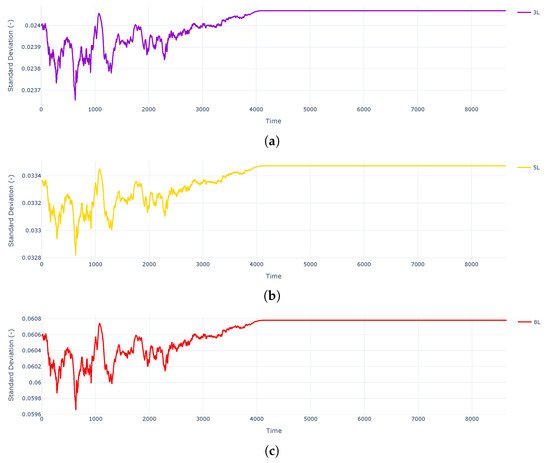
Figure 9.
Evolution of the normalized standard deviation throughout a day: (a) 3L change on standard deviation; (b) 5L change on standard deviation; (c) 8L change on standard deviation.
Even though they follow the same trend, the variance does differ significantly according to the number of Latent GPs. This does affect which values are included as part of the expected behavior of the turbine, as can be seen in Figure 10, during the expected behavior of the turbine. That means that distributionally, there is a higher probability of having the interval of the real value.
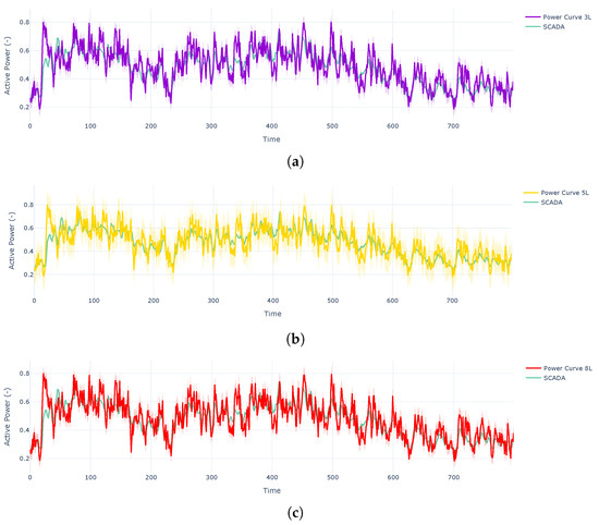
Figure 10.
Predictions during normal behavior of a turbine. (a) Predictions on normal behavior 3L. (b) Predictions on normal behavior 5L. (c) Predictions on normal behavior with 8L.
It is noticeable that using , the real SCADA value is more likely to be included in the credible intervals. This is because, apparently, variance seems to be higher when using a higher amount of latent spaces. Therefore, as seen in Figure 10, it covers most of the real values compared with the other L parameters.
As can be seen in Figure 11, the reconstruct is affected by the wind speed; nonetheless, the predictions are noisier than before. This means that the reported wind speed was noisier during the underperformance.
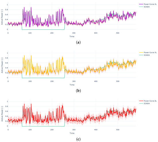
Figure 11.
Reconstruction during the stop of a turbine. (a) Predictions during a stop with 3L. (b) Predictions during a stop with 5L. (c) Predictions during a stop with 8L.
This provides an idea of how the probability distribution of the expected behavior might work. Based on this, probabilities of under-performance can be computed per timestep as well, considering how the variability changes throughout time using thresholding methods and definitions of underperformance.
3.4. Posterior Correlations
As the amount of L goes up, theoretically, the estimation of the model can capture more complex dependencies between tasks. It is expected that as L goes up, certain spurious correlations stabilize. The behavior was seen on certain specific turbines that were considered a priori not to be correlated, as shown in Figure 12.
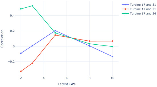
Figure 12.
Correlations according to the number of Latent Spaces.
Because of the behavior seen in the last section, the interpretation of the posterior correlations will be performed on the model of . As can be seen in the last section, this model provides the probability distribution, where the highest amount of points under stable behavior are still in the confidence interval of expected behavior. From these correlations, it is expected to be able to provide straightforward physical interpretations.
From the initial thoughts seen in Figure 13 and Figure 14, one can speculate that turbines in the wake are usually highly correlated (in magnitude, either positive or negative) with a turbine in the free-flow and turbines that are placed similarly under wake conditions. This means a similar distance and placement as the turbine itself, but not necessarily in the same neighborhood. This can be further confirmed when checking the heatmap with the correlations in Figure 15.
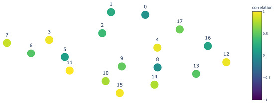
Figure 13.
Correlations for Turbine 11.
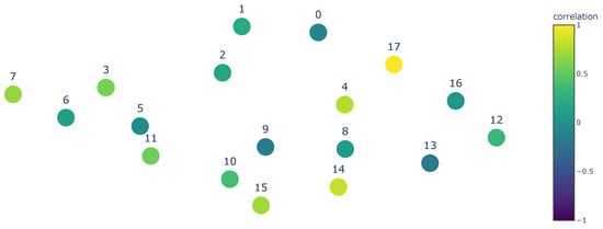
Figure 14.
Correlations for Turbine 17.
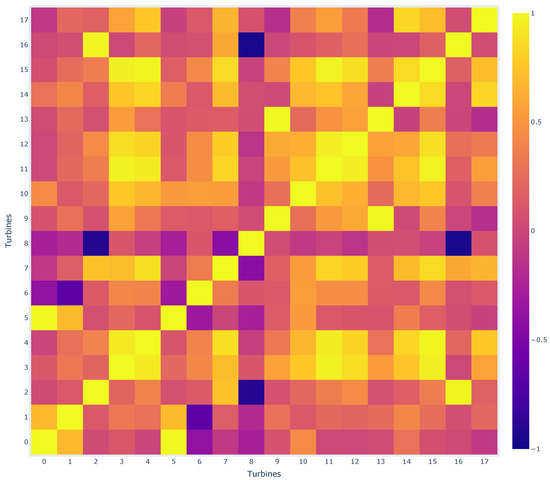
Figure 15.
Correlation matrix of the shown turbines.
Even though it was expected for the correlations to move according to input, this behavior was not seen; the correlations converged to the initial estimated task correlations. This behavior can be seen in Figure 16, where it is noticeable that the change throughout time is negligible.
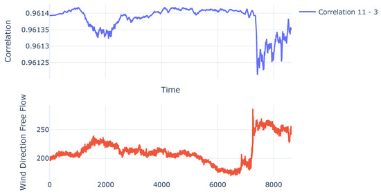
Figure 16.
Behavior of the correlation throughout a day.
3.5. Behavior During a Fault
The method was applied to predict the entirety of the dataset, in spite of steady or non-steady behavior. When using the method to check possible underperformances, there was a particular case that was highlighted. This case is highlighted given the fact that it was confirmed as abnormal behavior by the wind farm operator. This behavior was also reported by [10] using the same dataset. This case calls attention to the fact that it was also reported by the wind farm operator.
This abnormal behavior is based on a faulty anemometer, given that the wind speeds that are reported are expected to be higher than what was perceived. As a use case to detect faulty behavior, it will be contrasted with the IEC-suggested binning. Therefore, according to the anemometers’ data, the production should have been higher; nonetheless, most of the timesteps were outside the bounds. As can be seen in Figure 17, the proposed methodology is more sensitive and presents less uncertainty compared to the variance observed in the data. This can be attributed to the fact that farm-wide observations were used, thus, better estimating the covariances.
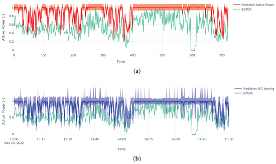
Figure 17.
Time series during a faulty anemometer. (a) Predictions with proposed model. (b) Predictions using IEC binning.
4. Discussion
This research presents a methodology that not only predicts active power using high-frequency data but also provides an estimation of the uncertainty via probabilistic methods. This approach’s main novelty is the combination of prior information from power curves combined with autoregressive modeling with Kernels. Due to this, the method produces credible intervals, correlation structures, and interpretable variance estimates. The nature of the methodology permits the probabilistic calculation of more complex assumptions related to the distribution of active power dependent on environmental parameters. This adds to the already existing procedures based on power curves, which make assumptions based on the Gaussian Distribution.
The inclusion of the inferential framework, which profits from environmental and park-wide variables, permits a correction of the power curve. This correction enforces the correlation between turbines, which makes a more informed power curve, including past information. Nonetheless, it is necessary to highlight that if the anemometers provide poor measurements, the correction from the informed past inputs will be very noisy.
The main novelty that can be highlighted is the fact that the methodology presented here is flexible towards the mean function, therefore permitting different models of the same process. This permits using complex machine learning methodologies, which might provide a better prediction than the one presented here to be used as part of the fitting process. With the use of the latter, it is possible to add the learning of the covariance as part of the algorithm. In addition to that, physics functions can be used as mean functions, therefore opening the possibility of using very accurate ensembles on the mean functions as well.
It is important to highlight the efficient use of data that the method provides, for example, obtaining in-depth results with a significantly low amount of data (15 days). This suggests that it is possible to, with the help of Kernel machines and probabilistic methods, learn complex behavior in the data.
4.1. Uncertainty Measures
As can be seen in Figure 9, Figure 10 and Figure 11, the uncertainty on the posterior active power is computable but dependent on the latent spaces. Further research should focus on how the mean function impacts the uncertainty, as assessed by the Gaussian Process Regression, as discussed in [39]; this information has effects on the Kernel parameters and the posterior distribution. It is necessary, therefore, as discussed further, to provide an accurate mean function.
Another topic to be discussed is that throughout this methodology, like in [11,12], the distribution of the outputs is assumed to be a Conditional Gaussian. The incorporation of certain knowledge on the prior information on the Gaussian Process Regression could give more reliable uncertainty estimations. By this, it is intended to suggest the inclusion of information about the wind speed, which is hypothesized to follow a Weibull distribution [33].
Using probability distribution transformations based on the power curve, it is possible to provide an analytical distribution that permits better uncertainty computations. This can be done via the transformation of the probability distribution of the assumed Weibull. Going back to the power curve formulation, one could have
Assuming that V follows a Weibull distribution and the rest of the coefficients are constant, via the transformation of the distribution explained in [40],
Nonetheless, this ignores that the probability distribution should also have the constraints of the cut-in wind speed and rated speed. Therefore, it is necessary to come to a more rigorous mapping of the possible probability distribution, instead of assuming a Gaussian Distribution.
In addition, as said before, there is a possibility that the variability of the system on the posterior distribution is inflated. This is because certain covariances could provide spurious relationships, which can inflate the variance estimates. Nonetheless, this should not be significantly affect.
This analytical way to measure uncertainty constitutes a method that is completely based on SCADA data and can be used independently of the model used for the SCADA indicators. Here, it is only presented on the manufacturer’s power curve; nonetheless, it can easily be adapted to make inferences on MLPs and LSTMs. This makes the model less dependent on assumptions from the mean function.
4.2. Lagged Input Corrected Power Curve
As discussed earlier, since during the optimization of the W matrix the lagged inputs are used, it could be considered that this matrix corrects the power curve with the temporal information. Nonetheless, this requires intensive data-driven steps that do not give a definite universal answer on how to correct the power curve with the past observations. Therefore, one can only conclude that it is possible to do it in a data-driven way, with complex vectorial interactions, with the difference that in the end, these interactions can be traced and further interpreted.
On top of the aforementioned correction based on temporal inputs, the calculation of the variance is also lagged input aware. Overall, the model will have a great profit from using both past (or lagged) inputs and power curve information, in case there are forecasts of the wind speed at the anemometer height. Also, in further sections, it will be discussed that one can find a correcting function for the anemometer-reported wind speed when the turbine is down.
Based on the evidence presented here, there is a result that seems counter-intuitive according to the principles of GPR modeling. The result suggests that with a lower amount of Latent GPs (L), the predictive power improves. It would be expected that with a higher amount of L, the variability of the system is better modeled.
4.3. Notes on the Mean Function
The mean function presented here, based on the power curve, is one of the most commonly used in research; nonetheless, better mean functions can be proposed. Under this framework, it is possible to consider more complex non-linear functions, such as the ones proposed by [13] or mean functions with more complex algebraic structures, such as [17], which could have a better posterior distribution estimation. For further work, these mean functions and how to extract the features for the Kernel inference can be explored.
The flexibility of the mean function also permits transparency if required. Unless Black-Box mean functions are used, one could control how the mean function is parametrized. Therefore, corrections of the power curve based on yaw misalignment, such as the ones presented in [41], can be included as part of a deterministic mean function. On top of the aforementioned, other corrections based on lagged inputs that are not inherent to the matrix W can be proposed, such as moving averages of the power curve values. Apart from the latter, environmental power curves such as the ones proposed in [12] can also be included, given that they seem to have a similar performance. Further work should focus on these contributions that can be obtained from other mean functions.
4.4. Park-Wide Correlations
The model offers park-wide correlations that can be helpful when having a turbine down. It was found that when a turbine is down, the data from the anemometer could be unreliable or noisy; therefore, this shows that based on the task correlations, it is possible to think of a function that corrects the anemometer-reported value. One could speculate on a mapping of the way
where would represent the wind speed at another correlated turbine, and m is a mapping that could be linear or non-linear. It can even be expressed as a function of the n largest correlated turbines. This could be used to calculate possible energy losses, with less noisy behaviors.
4.5. Other SCADA Indicators
As discussed in [13], one can create deterministic functions of all the SCADA indicators. The methodology here can be extended to the rotor speed, generator speed, and current. This would estimate the correlations between the turbines and other behaviors present in the SCADA system. The exploration here would also pose the challenge of mean functions that also produce several tasks, given that multi-target modeling is suggested when modeling these SCADA performance indicators.
5. Conclusions
This study presents a statistical approach for predicting expected active power and estimating associated uncertainties. It is important to note that the methodology is flexible enough to incorporate different estimations of the active power, also enforcing a relationship in the posterior distribution. This can be generalized to almost any algebraic structure that is used in machine learning. Based on the results, it has also been proposed to provide further research on how the mean functions can leverage better farm-wide and auto-regressive information. The model provides valuable tools such as uncertainty bounds and posterior correlations, which can inform real-time monitoring and control strategies.
The methodology presented here marginally improves the prediction provided by the power curve. Knowing this, this methodology can be expanded to machine learning functions, which should be explored in further work. The measure of uncertainty on pre-trained models for SCADA indicators can be expanded by using the proposed methods. The method here also has the particularity that it relies entirely on SCADA data, and it does not have any assumptions or corrections; it constitutes a method that, independently of how the SCADA indicator is predicted, will calculate uncertainty. Nonetheless, it is important to highlight that this not only contributes to uncertainty estimation of power curves but also permits flexibility in plugging in other mean functions, which permits further research on SCADA-based wind farm analytics.
The methodology proposes a way to use both farm-wide and autoregressive information, using temporal inputs and assuming that the covariance matrix models the farm-wide information in the probability distribution. The use of this information improves the prediction under dominant wind directions up to a 5%, but overall improves it 1%. A very basic, intuitive physical explanation was provided based on the highest reliable amount of Latent Spaces in the Gaussian Process. Further research using the methodology with other priors is necessary and could significantly improve the accuracy.
Author Contributions
Conceptualization, F.J.J.Á.; Formal analysis, F.J.J.Á.; Writing—original draft, F.J.J.Á.; Writing—review & editing, A.N. and J.H.; Supervision, T.V., P.J.D. and J.H.; Funding acquisition, A.N. and J.H. All authors have read and agreed to the published version of the manuscript.
Funding
This research received no external funding.
Data Availability Statement
Requests to access the datasets should be directed to corresponding author.
Acknowledgments
The authors would like to acknowledge the Energy Transition Funds for their support through the POSEIDON and BeFORECAST projects from FOD Belgium.
Conflicts of Interest
The authors declare that the research was conducted in the absence of any commercial or financial relationships that could be construed as a potential conflict of interest.
Abbreviations
The following abbreviations are used in this manuscript:
| SCADA | Supervisory Control and Data Acquisition |
| GP | Gaussian Process |
| IMC | Intrinsic Model of Coregionalization |
| LMC | Linear Model of Coregionalization |
| MLP | Multi-Layer Perceptron |
| LSTM | Long Short-Term Memory |
| GPR | Gaussian Process Regression |
| MAE | Mean Absolute Error |
| RMSE | Root Mean Squared Error |
| Coefficient of determination | |
| MAPE | Mean Absolute Percentage Error |
| SVGP | Stochastic Variational Gaussian Process |
| ELBO | Evidence Lower Bound |
| KL divergence | Kullback–Leibler Divergence |
References
- Manwell, J.; McGowan, J.; Rogers, A. Wind Energy Explained: Theory, Design and Application; Wiley: Hoboken, NJ, USA, 2010. [Google Scholar]
- Khamees, A.K.; Abdelaziz, A.Y.; Eskaros, M.R.; Alhelou, H.H.; Attia, M.A. Stochastic Modeling for Wind Energy and Multi-Objective Optimal Power Flow by Novel Meta-Heuristic Method. IEEE Access 2021, 9, 158353–158366. [Google Scholar] [CrossRef]
- Yang, W.; Tavner, P.J.; Crabtree, C.J.; Feng, Y.; Qiu, Y. Wind turbine condition monitoring: Technical and commercial challenges. Wind Energy 2014, 17, 673–693. [Google Scholar] [CrossRef]
- Mücke, T.A.; Wächter, M.; Milan, P.; Peinke, J. Langevin power curve analysis for numerical wind energy converter models with new insights on high frequency power performance. Wind Energy 2015, 18, 1953–1971. [Google Scholar] [CrossRef]
- Lydia, M.; Kumar, S.S.; Selvakumar, A.I.; Prem Kumar, G.E. A comprehensive review on wind turbine power curve modeling techniques. Renew. Sustain. Energy Rev. 2014, 30, 452–460. [Google Scholar] [CrossRef]
- Uluyol, O.; Parthasarathy, G.; Foslien, W.; Kim, K. Power curve analytic for wind turbine performance monitoring and prognostics. In Proceedings of the Annual Conference of the PHM Society, Montreal, QC, Canada, 25–29 September 2011; Volume 3. [Google Scholar]
- Shokrzadeh, S.; Jozani, M.J.; Bibeau, E. Wind turbine power curve modeling using advanced parametric and nonparametric methods. IEEE Trans. Sustain. Energy 2014, 5, 1262–1269. [Google Scholar] [CrossRef]
- Schlechtingen, M.; Santos, I.F.; Achiche, S. Using Data-Mining Approaches for Wind Turbine Power Curve Monitoring: A Comparative Study. IEEE Trans. Sustain. Energy 2013, 4, 671–679. [Google Scholar] [CrossRef]
- Gonzalez, E.; Stephen, B.; Infield, D.; Melero, J.J. On the use of high-frequency SCADA data for improved wind turbine performance monitoring. J. Phys. Conf. Ser. 2017, 926, 012009. [Google Scholar] [CrossRef]
- Daenens, S.; Vervlimmeren, I.; Verstraeten, T.; Daems, P.J.; Nowé, A.; Helsen, J. Power prediction using high-resolution SCADA data with a farm-wide deep neural network approach. J. Phys. Conf. Ser. 2024, 2767, 092014. [Google Scholar] [CrossRef]
- Jara Ávila, F.; Verstraeten, T.; Vratsinis, K.; Nowé, A.; Helsen, J. Wind Power Prediction using Multi-Task Gaussian Process Regression with Lagged Inputs. J. Phys. Conf. Ser. 2023, 2505, 012035. [Google Scholar] [CrossRef]
- Ávila, F.J.; Daenens, S.; Vervlimmeren, I.; Verstraeten, T.; Helsen, J. Turbine-Level Possible Power Prediction using Farm-Wide Spatial Information through Similarity-Based Multivariate Gaussians. J. Phys. Conf. Ser. 2024, 2767, 062031. [Google Scholar] [CrossRef]
- Meyer, A. Multi-target normal behaviour models for wind farm condition monitoring. Appl. Energy 2021, 300, 117342. [Google Scholar] [CrossRef]
- Liu, Z.; Gao, W.; Wan, Y.H.; Muljadi, E. Wind power plant prediction by using neural networks. In Proceedings of the 2012 IEEE Energy Conversion Congress and Exposition (ECCE), Raleigh, NC, USA, 15–20 September 2012; pp. 3154–3160. [Google Scholar] [CrossRef]
- St. Martin, C.M.; Lundquist, J.K.; Clifton, A.; Poulos, G.S.; Schreck, S.J. Wind turbine power production and annual energy production depend on atmospheric stability and turbulence. Wind Energy Sci. 2016, 1, 221–236. [Google Scholar] [CrossRef]
- Wagner, R.; Courtney, M.; Gottschall, J.; Lindelöw-Marsden, P. Accounting for the speed shear in wind turbine power performance measurement. Wind Energy 2011, 14, 993–1004. [Google Scholar] [CrossRef]
- Daenens, S.; Verstraeten, T.; Daems, P.J.; Nowé, A.; Helsen, J. Spatio-Temporal Graph Neural Networks for Power Prediction in Offshore Wind Farms Using SCADA Data. Wind Energy Sci. Discuss. 2024, 10, 1137–1152. [Google Scholar] [CrossRef]
- Rasmussen, C.E.; Williams, C.K.I. Gaussian Processes for Machine Learning; The MIT Press: Cambridge, MA, USA, 2006. [Google Scholar]
- Hensman, J.; Fusi, N.; Lawrence, N.D. Gaussian Processes for Big Data. arXiv 2013, arXiv:1309.6835. [Google Scholar]
- Fortuin, V.; Strathmann, H.; Rätsch, G. Meta-Learning Mean Functions for Gaussian Processes. arXiv 2019, arXiv:1901.08098. [Google Scholar]
- Cotton, P. Microprediction: Building an Open AI Network; MIT Press: Cambridge, MA, USA, 2022. [Google Scholar]
- Zhang, J.; Jain, R.; Hodge, B.M. A data-driven method to characterize turbulence-caused uncertainty in wind power generation. Energy 2016, 112, 1139–1152. [Google Scholar] [CrossRef]
- Daems, P.J.; Peeters, C.; Matthys, J.; Helsen, J. Fleet-wide analytics on field data targeting condition and lifetime aspects of wind turbine drivetrains. Forsch. Im Ingenieurwesen 2023, 87, 285–295. [Google Scholar] [CrossRef]
- Daems, P.J.; Guo, Y.; Sheng, S.; Peeters, C.; Guillaume, P.; Helsen, J. Gaining Insights in Loading Events for Wind Turbine Drivetrain Prognostics; American Society of Mechanical Engineers: New York, NY, USA, 2020; Volume 84249. [Google Scholar]
- Jammalamadaka, S.R.; SenGupta, A. Topics in Circular Statistics; World Scientific: Singapore, 2001. [Google Scholar] [CrossRef]
- Bonilla, E.V.; Chai, K.; Williams, C. Multi-task Gaussian Process Prediction. In Proceedings of the Advances in Neural Information Processing Systems, Vancouver, BC, Canada, 3–6 December 2007; Platt, J., Koller, D., Singer, Y., Roweis, S., Eds.; Curran Associates, Inc.: Red Hook, NY, USA, 2007; Volume 20. [Google Scholar]
- van der Wilk, M.; Dutordoir, V.; John, S.; Artemev, A.; Adam, V.; Hensman, J. A Framework for Interdomain and Multioutput Gaussian Processes. arXiv 2020, arXiv:2003.01115. [Google Scholar]
- Chai, K.M.A. Multi-Task Learning with Gaussian Processes. Ph.D. Thesis, University of Edinburgh, Edinburgh, UK, 2010. [Google Scholar]
- David, M.; Blei, A.K.; McAuliffe, J.D. Variational Inference: A Review for Statisticians. J. Am. Stat. Assoc. 2017, 112, 859–877. [Google Scholar] [CrossRef]
- Titsias, M.; Lawrence, N.D. Bayesian Gaussian Process Latent Variable Model. In Proceedings of the Thirteenth International Conference on Artificial Intelligence and Statistics, Sardinia, Italy, 13–15 May 2010; Teh, Y.W., Titterington, M., Eds.; Chia Laguna Resort; Volume 9, Proceedings of Machine Learning Research. pp. 844–851. [Google Scholar]
- Matern, B. Spatial Variation; Lecture Notes in Statistics; Springer: New York, NY, USA, 1986. [Google Scholar]
- Abramowitz, M.; Stegun, I. Handbook of Mathematical Functions: With Formulas, Graphs, and Mathematical Tables; Applied mathematics series; Dover Publications: Garden City, NY, USA, 1965. [Google Scholar]
- Ding, Y. Data Science for Wind Energy; CRC Press: Boca Raton, FL, USA, 2020. [Google Scholar]
- Ackermann, T. Wind Power in Power Systems; Wind Engineering; John Wiley & Sons, Ltd.: Hoboken, NJ, USA, 2005; pp. 1–692. [Google Scholar]
- Hensman, J.; de Matthews, A.G.; Ghahramani, Z. Scalable Variational Gaussian Process Classification. In Proceedings of the International Conference on Artificial Intelligence and Statistics, Reykjavic, Iceland, 22–25 April 2014. [Google Scholar]
- Kingma, D.P.; Ba, J. Adam: A Method for Stochastic Optimization. arXiv 2017, arXiv:1412.6980. [Google Scholar]
- Khodamoradi, A.; Denolf, K.; Vissers, K.; Kastner, R.C. ASLR: An Adaptive Scheduler for Learning Rate. In Proceedings of the 2021 International Joint Conference on Neural Networks (IJCNN), Shenzhen, China, 18–22 July 2021; pp. 1–8. [Google Scholar] [CrossRef]
- Salimbeni, H.; Eleftheriadis, S.; Hensman, J. Natural Gradients in Practice: Non-Conjugate Variational Inference in Gaussian Process Models. arXiv 2018, arXiv:1803.09151. [Google Scholar]
- Guan, Y.; Li, D.; Xue, S.; Xi, Y. Feature-fusion-kernel-based Gaussian process model for probabilistic long-term load forecasting. Neurocomputing 2021, 426, 174–184. [Google Scholar] [CrossRef]
- Wackerly, D.; Mendenhall, W.; Scheaffer, R. Mathematical Statistics with Applications; Cengage Learning: Singapore, 2014. [Google Scholar]
- Astolfi, D.; Pandit, R.; Lombardi, A.; Terzi, L. Diagnosis of wind turbine systematic yaw error through nacelle anemometer measurement analysis. Sustain. Energy Grids Netw. 2023, 34, 101071. [Google Scholar] [CrossRef]
Disclaimer/Publisher’s Note: The statements, opinions and data contained in all publications are solely those of the individual author(s) and contributor(s) and not of MDPI and/or the editor(s). MDPI and/or the editor(s) disclaim responsibility for any injury to people or property resulting from any ideas, methods, instructions or products referred to in the content. |
© 2025 by the authors. Licensee MDPI, Basel, Switzerland. This article is an open access article distributed under the terms and conditions of the Creative Commons Attribution (CC BY) license (https://creativecommons.org/licenses/by/4.0/).