1. Introduction
With the accelerating global energy transition and the continuous growth of natural gas consumption, Underground Gas Storage (UGS) facilities have become increasingly vital for regulating seasonal supply-demand imbalances, ensuring energy security, and enhancing market operational flexibility [
1,
2,
3,
4]. UGS facilities are typically constructed in depleted oil and gas reservoirs, aquifers, or salt caverns, enabling large-scale natural gas storage through high-pressure injection and allowing for rapid production during peak demand or emergencies. However, the pursuit of larger storage capacities and higher operational safety poses new geomechanical and monitoring challenges to existing reservoir structures [
5,
6,
7,
8].
Converting mature oilfields, particularly depleted oil and gas reservoirs, into underground gas storage (UGS) facilities is an important and increasingly common approach for UGS development. Depleted reservoirs offer several advantages for such conversions, including well-characterized geological conditions, the potential for reutilizing existing infrastructure—especially wells—an abundance of geological and engineering data accumulated during hydrocarbon exploration and production, and a preliminary validation of caprock sealing integrity [
9,
10,
11,
12]. However, compared to rigid storage media such as salt caverns, depleted reservoirs exhibit significant evolution of reservoir pressure fields and in situ stress fields during long-term cyclic injection and production operations. These dynamic changes may result in the reactivation of pre-existing faults and the propagation of microfractures through the caprock, thereby increasing the risk of gas leakage and compromising the overall sealing capacity of the storage system. This risk is particularly pronounced when the original reservoir was designed for liquid hydrocarbon containment rather than for gas storage, where the sealing conditions for gaseous phases impose more stringent requirements. These challenges highlight the necessity for continuous geomechanical monitoring and integrity assessments in reservoir-based UGS facilities [
9,
13,
14].
In recent years, microseismic monitoring has been widely adopted as a high-resolution and real-time sensing technology for detecting subsurface stress perturbations. It has found broad application in reservoir development, hydraulic fracturing, deep geothermal exploitation, CO
2 geological sequestration, coal mining, and UGS integrity monitoring [
15,
16,
17,
18]. By capturing low-magnitude events induced by pressure disturbances during injection and production, microseismic monitoring provides real-time insights into fault slip, fracture propagation, and reservoir deformation processes. Compared with traditional downhole pressure or deformation monitoring, microseismic techniques are non-intrusive, offer excellent spatial characterization capabilities, and provide dynamic and timely responses, making them an important supplementary tool for UGS safety monitoring [
19,
20].
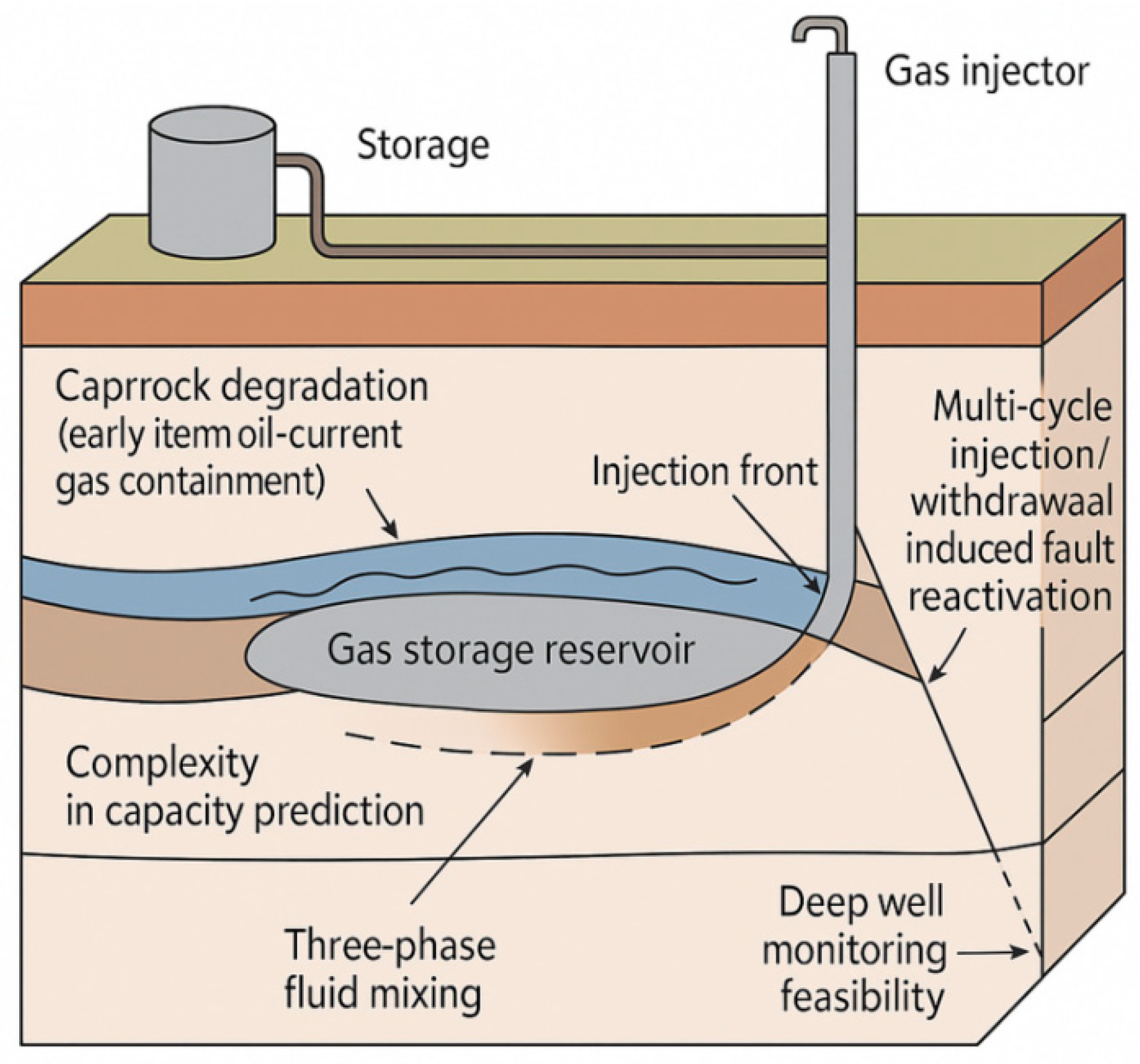
Figure 1 illustrates the various geological and engineering challenges that may arise during the conversion of a hydrocarbon reservoir into an underground gas storage (UGS) facility. First, the caprock of the original reservoir may have experienced mechanical fatigue and degradation due to long-term hydrocarbon production, compromising its integrity. In addition, the absence of an original gas cap structure raises concerns regarding the dynamic sealing capacity of the caprock after gas injection, which requires further validation [
21]. Secondly, the mixing of multiphase fluids (e.g., original oil, water, and injected gas) within the reservoir complicates the prediction of gas mobility and the estimation of total storage capacity [
11]. Furthermore, cyclic pressure variations during injection and production may induce fault reactivation, increasing leakage risks [
9,
13,
14]. The figure also emphasizes challenges such as three-phase fluid front propagation during gas injection, the technical feasibility of deep-well microseismic monitoring, and the need for accurate reservoir capacity evaluation [
22]. Through this schematic, the complexity of the geological–mechanical–monitoring coupling mechanisms in UGS projects can be intuitively understood, highlighting the significance of deploying high-resolution microseismic monitoring systems [
23,
24].
In this study, the Jidong Oilfield No. 2 Underground Gas Storage (UGS) facility in Northern China was selected as the test site. A 90-day microseismic monitoring experiment was conducted during actual injection and production operations in the converted reservoir. A combined surface and shallow borehole microseismic monitoring system was deployed to record microseismic activity within the deep reservoir. The objectives of the study were: (1) to evaluate the feasibility of microseismic monitoring observation geometry in deep, low signal-to-noise ratio environments; (2) to detect low-magnitude injection-induced events using the short-term average to long-term average (STA/LTA) algorithm combined with manual phase picking and beamforming techniques; and (3) to assess the limitations of the current monitoring system deployment and processing workflow, and to propose technical optimizations for future long-term monitoring facility installment of UGS facilities.
These faults may compromise the sealing integrity of the caprock, posing potential pathways for gas leakage or zones for microseismic event initiation. Therefore, dynamic monitoring and evaluation of fault zone sealing capacity and reactivation risk are urgently required.
2. Geological Background
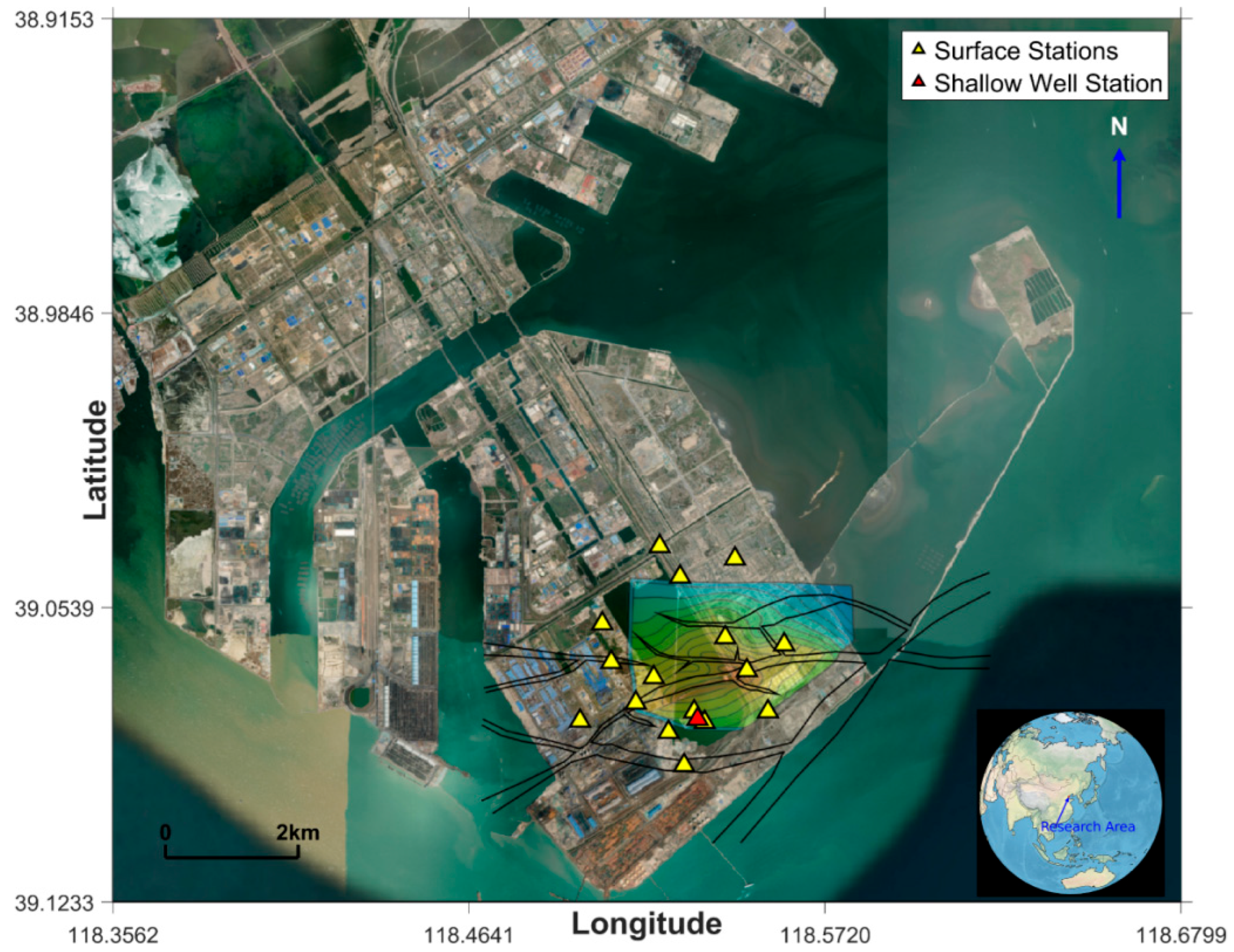
The Jidong Oilfield No. 2 Underground Gas Storage (UGS) facility is located in the Nanpu Sag of the Huanghua Depression, in the northern Bohai Bay Basin, nearshore in Tangshan City, Hebei Province. The site features flat terrain and extensive tidal flats, with seawater depths ranging from 0 to 10 m, providing favorable geographical conditions for the construction of artificial islands and the deployment of seismic monitoring systems.
Structurally, the M block is located in the western segment of the No. 3 anticline in the Nanpu Sag and represents a faulted anticline structure formed by the superimposed control of early near east–west-trending faults and later NE–SW-trending faults. The structural high is situated near Well NP3-80, providing a stable structural trap favorable for natural gas accumulation and storage, thus offering a solid geological basis for UGS conversion. The regional tectonic setting is complex, lying within the tectonically active zone of the Huanghua Depression. It has been influenced by multiple phases of extensional and strike-slip tectonic activity since the Cenozoic, resulting in a dense fault network with frequent reactivation events [
25,
26].
The target reservoir is located in the Shahejie Formation (Es1), characterized by a stable and well-developed anticlinal structural trap [
27]. Well logging and core data indicate that the Es1 reservoir has an average effective thickness of approximately 73.7 m. It is overlain by a grey mudstone caprock exceeding 227 m in thickness, with the uppermost ~90 m forming the primary seal, constituting a high-quality reservoir-caprock assemblage. Seismic interpretation has identified a total of 11 major faults within the area, among which seven faults penetrate the top boundary of the reservoir.
3. Monitoring System and Data Processing
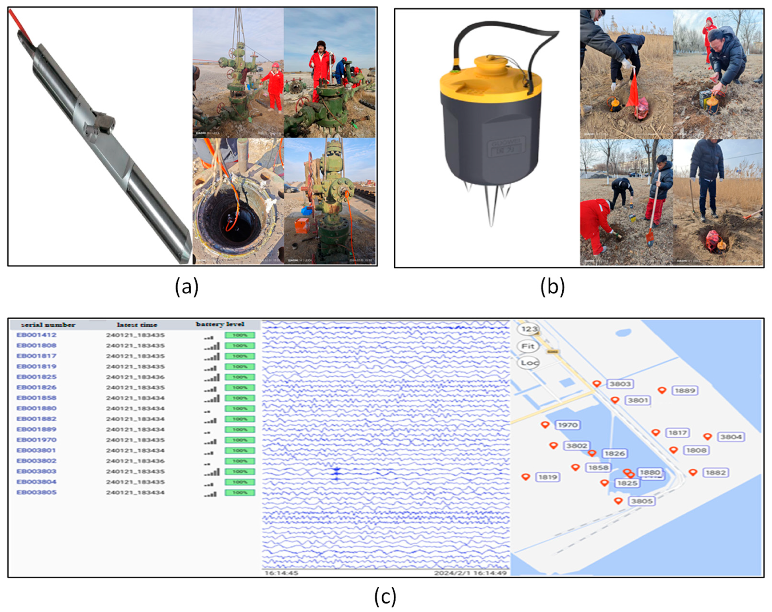
To monitor the dynamic response of the reservoir stress field during injection and production operations at the No. 2 UGS facility, a microseismic monitoring system combining surface and shallow borehole stations was deployed, consisting of 16 mobile surface stations and 1 downhole station (
Table 1). This system integrates surface geophones installed on artificial islands with shallow borehole sensors deployed within existing wellbores, enabling continuous real-time acquisition of microseismic signals under deep, high-attenuation, and low signal-to-noise ratio conditions. The objective of this setup was to evaluate the applicability of surface and shallow borehole monitoring, in addition to deep borehole monitoring, for this UGS facility. For instance, if only the shallow borehole sensors detect clear microseismic events while the surface stations exhibit poor signal response, it would indicate that long-term monitoring could rely primarily on shallow and deep borehole deployments. Conversely, if neither the surface nor shallow borehole stations can capture distinct microseismic events (e.g., clear first arrivals), it would suggest that long-term monitoring should rely exclusively on deep borehole systems.
Station Deployment and Instrumentation: A total of 16 high-sensitivity three-component short-period seismometers were deployed, evenly distributed on the artificial island, with an inter-station spacing of approximately 300–600 m, covering the main structure of the gas storage facility. Additionally, one shallow-well monitoring device was installed inside Well 3657, with the sensor deployed at a depth of 150 m (
Figure 2 and
Figure 3). All monitoring nodes are connected to the central data acquisition server via a 4G network to enable real-time data transmission. The designed monitoring network aperture is about 1–1.5 times the depth of the target reservoir (~4000 m), satisfying the spatial coverage requirements for horizontal event location and preliminary imaging, with focused coverage of critical areas such as the gas-water contact, caprock boundary, and fault zones.
Reservoir and Deployment Constraints: The original reservoir pressure was measured at approximately 40.17 MPa, with a formation temperature of 157 °C and a geothermal gradient of 3.2 °C per 100 m. Due to the temperature limitations of the shallow borehole geophones, the downhole sensors in the current experiment were deployed at depths shallower than 150 m. However, this shallow deployment led to limited geometric coupling between sensors and deep seismic sources, thereby reducing location accuracy and decreasing the detection capability for low-magnitude events. To overcome these limitations and enhance monitoring performance, we recommend future deployment of high-temperature and high-pressure resistant geophones (depth > 2500 m) in injection or adjacent observation wells. Such systems would improve signal acquisition near the reservoir, increase vertical resolution, and enable high-precision imaging of stress evolution, fracture propagation, and fault slip processes.
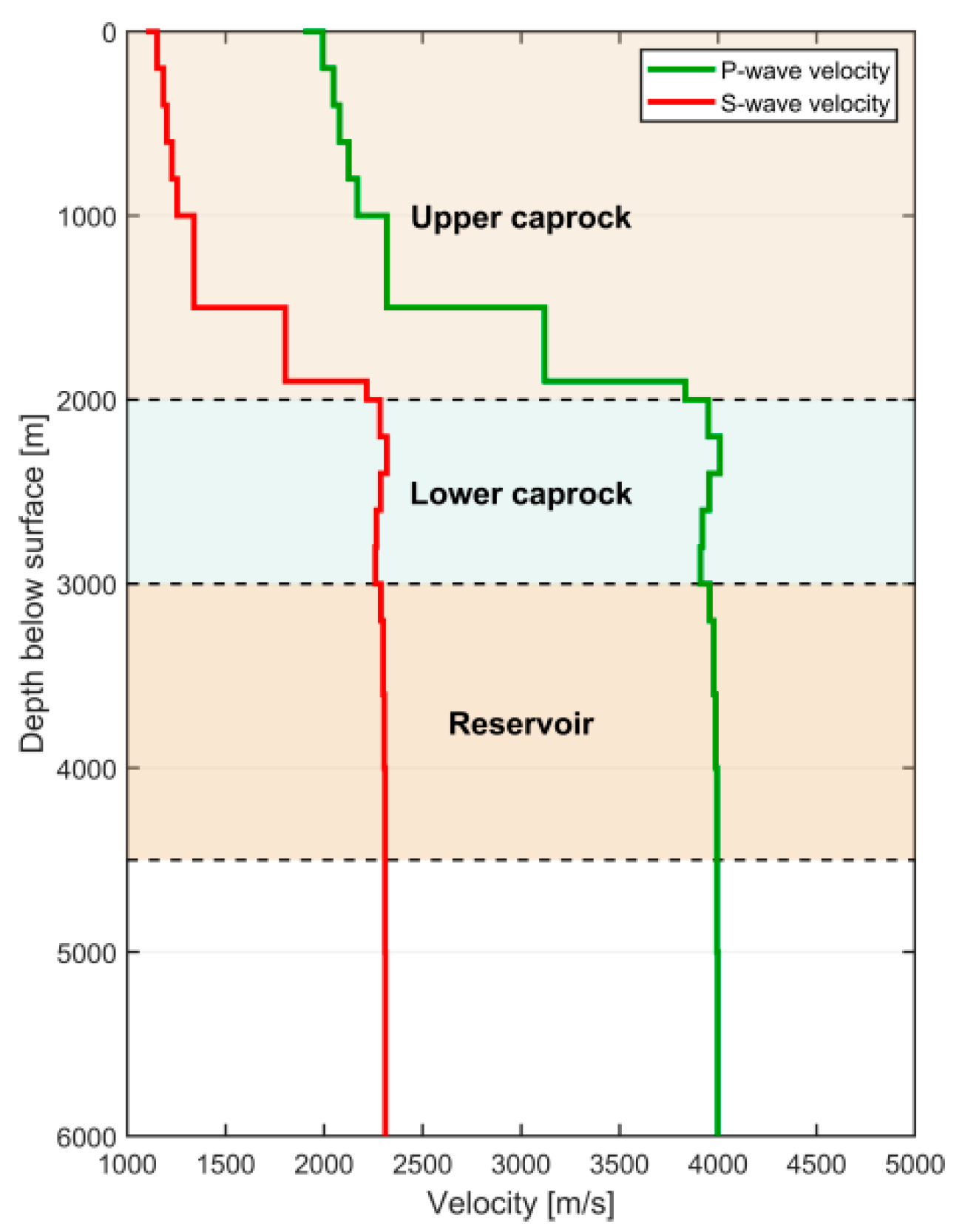
Velocity Model Construction and Travel-Time Table Calculation: Accurate event location relies on a reasonable subsurface velocity model. Based on dipole sonic logging and check-shot data from Wells PG2-QK1 and NP3-80, a one-dimensional horizontally isotropic layered velocity model was constructed. Near-surface low-velocity corrections were applied to account for the influence of shallow heterogeneities (
Figure 4). Travel-time computation employed the Wavefront Reconstruction Method (WFRM) to simulate the wave propagation paths from a grid of potential sources to each station, generating a three-dimensional travel-time table. Compared with traditional ray-tracing methods, WFRM better handles diffraction effects and shadow zones, improving the interpolation stability of the travel-time field and enhancing location accuracy.
Data Acquisition and Event Detection: The monitoring system operated continuously from 1 February to 30 April 2024, for a total of 90 days, recording three-component continuous waveform data at a sampling rate of 500 Hz. Data preprocessing included band-pass filtering, DC offset removal, and windowed segmentation. For low-magnitude event detection, a two-stage event detection process was adopted: (1) initial triggering was performed using the classical Short-Term Average/Long-Term Average (STA/LTA) algorithm, but under the low signal-to-noise ratio conditions of the study area, this method failed to detect most events; (2) beamforming analysis was then introduced, aligning and stacking waveforms across multiple stations to enhance the coherence of weak signals, thus improving the detection probability of “hidden” events in a noisy environment (The detailed derivation can be found in
Appendix A). The detected microseismic events were located using a grid-search algorithm based on the pre-generated WFRM travel-time field, minimizing the residuals between theoretical and observed travel times. Each event location was accompanied by an uncertainty estimate, mainly influenced by phase picking errors, station distribution geometry, and velocity model deviations.
4. Spatial and Temporal Distribution of Event Localisation
During the 90-day injection and production cycle at the No. 2 UGS facility, a large volume of three-component waveform data was continuously recorded by the surface and shallow borehole geophones. Despite the reservoir being buried at a depth of approximately 4000 m and the presence of strong environmental noise, 35 microseismic events (see
Appendix B) were successfully identified through enhanced processing using the beamforming method. A systematic analysis of the temporal distribution, injection-response characteristics, location errors, and spatial distribution of the events is presented below.
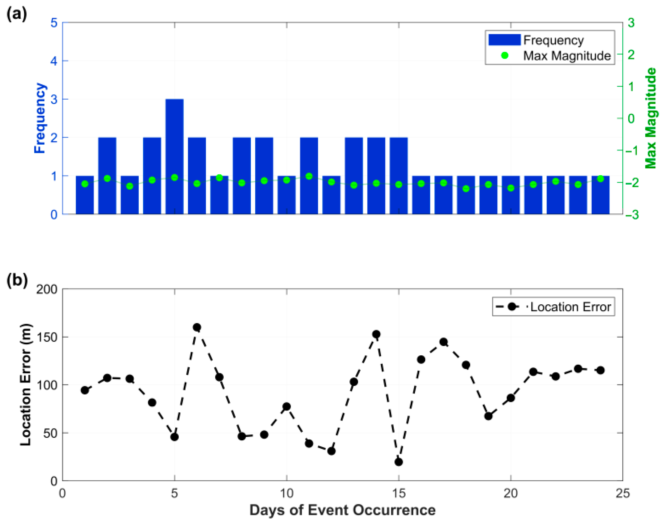
Temporal Distribution and Injection Response Characteristics: As shown in
Figure 5, the frequency of microseismic events exhibited a significant positive correlation with variations in wellhead pressure. During the initial monitoring period (1 February–6 March), the wellhead pressure of Well 3802 remained around 20 MPa, and no significant microseismic events were detected. After 7 March, as the injection pressure of Well 3802 increased to above 30 MPa, the first low-energy microseismic event was identified. Subsequently, beginning on 4 April, Wells 3804 and PG2-QK1 commenced gas injection, leading to an increase in the number of detected events. The overall trend indicates that microseismic activity is primarily controlled by stress perturbations in the reservoir, with no significant coupling to the daily gas injection volume. This behavior reflects that faults or microfractures near a critical stress state are more prone to slip, supporting the physical model of “stress-critical triggering mechanism”.
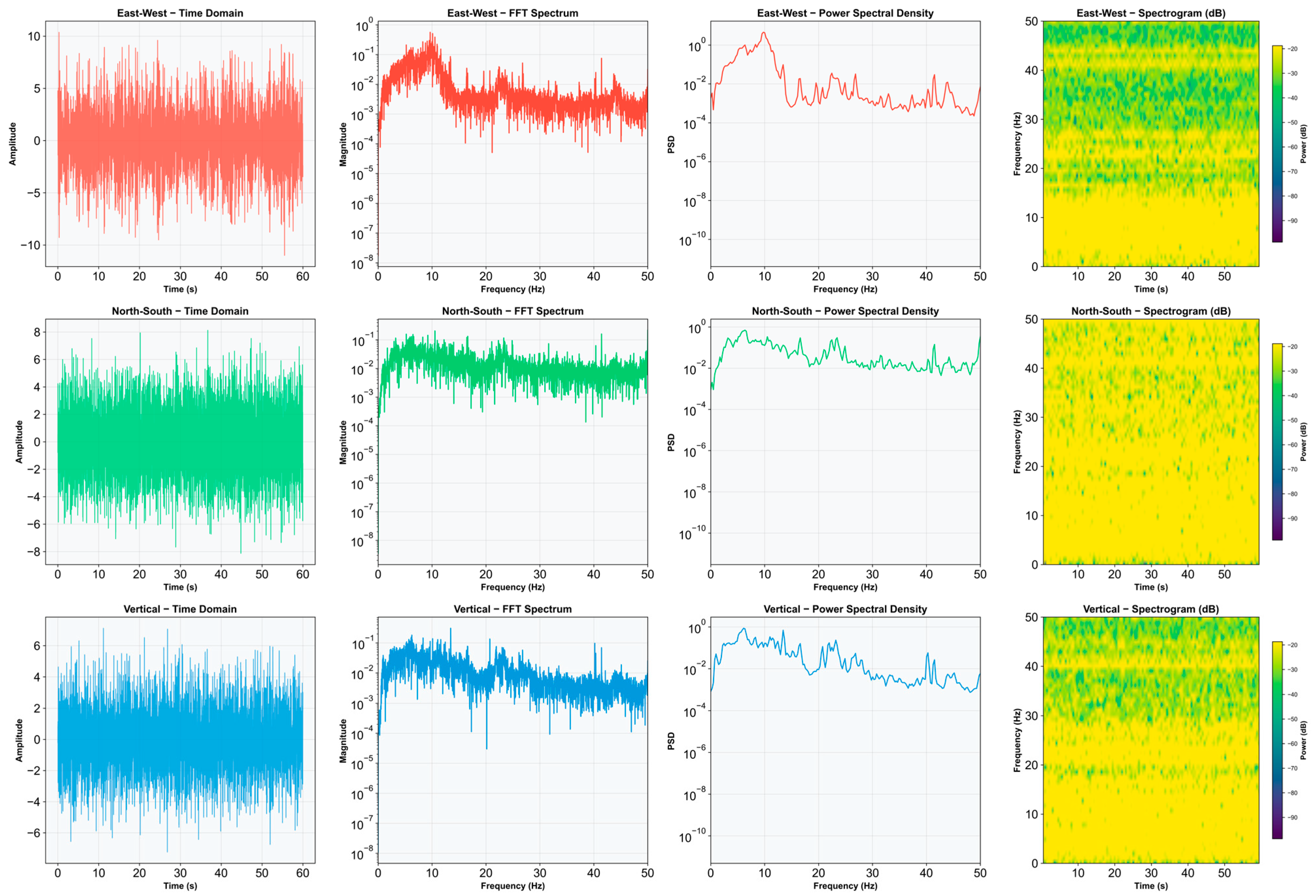
Waveform Characteristics of a Typical Invisible Event: To illustrate the waveform characteristics of a typical low-amplitude event, an analysis was conducted on an invisible microseismic event that occurred on 8 April 2024 (
Figure 6 and
Figure 7). The original amplitude of this event was extremely low (<1 μm/s), and it could not be detected by the conventional STA/LTA algorithm. However, after beamforming processing, which is a powerful processing technique renowned for its ability to pinpoint weak events by harnessing the superposition of waveforms. The stacked signals from multiple stations revealed clear phase coherence. Key features include: (1) in the raw waveform, P-wave and S-wave arrivals are nearly indistinguishable; (2) after beamforming processing, coherent wave peaks appear within the same time window; (3) the spectral content is dominated by frequencies between 10 and 20 Hz, consistent with the typical frequency range of small-scale fault slip events.
Hypocenter Location Error Analysis: All events were located using a grid search method based on the precomputed WFRM travel-time tables, and location errors were estimated. As shown in the statistical results in
Figure 8: (1) the minimum horizontal location error is approximately 19.7 m; (2) the maximum location error is about 160 m; (3) the average location error is around 87.5 m; (4) about 83% of the events have location errors greater than 70 m. The sources of error mainly include uncertainties in low signal-to-noise ratios of the events, insufficient vertical coverage of the receiving stations and inaccuracy in the velocity model.
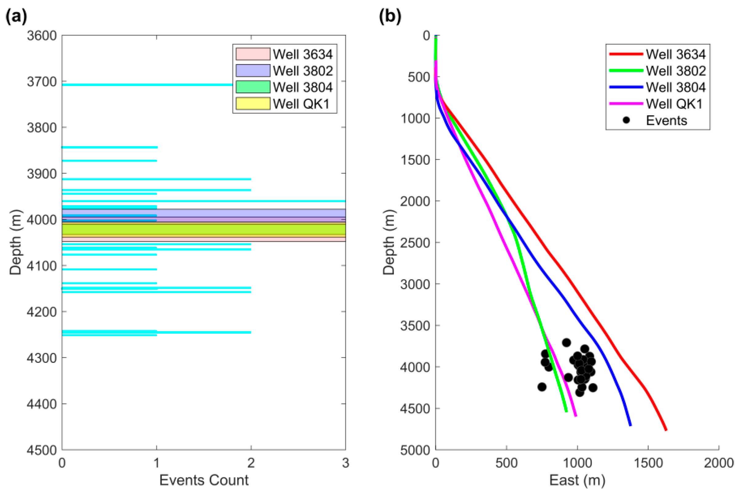
Spatial Distribution and Correspondence with Injection Intervals: The hypocenter depths of the recorded microseismic events were compared with the injection intervals of the corresponding wells (
Figure 9). Most events are horizontally located within 50–100 m of the main injection wells, indicating a clear spatial correlation. Vertically, however, the majority of events are systematically positioned 200–400 m above the injection intervals, suggesting a persistent shallow bias in the depth estimates. This bias is likely caused by the limited vertical resolution of the current monitoring system, which consists of surface and shallow borehole sensors located over 3.5 km above the reservoir (at approximately 4000 m depth). A representative vertical mislocation of ~300 m has critical implications: it may place events entirely within the overlying caprock rather than the reservoir, thereby complicating assessments of fault reactivation and caprock integrity. Given that the local caprock is only 100–200 m thick and fault slip zones often extend vertically for only a few tens to hundreds of meters, such location uncertainties are too large to reliably determine whether rupture occurs within or outside the sealing strata. Consequently, the current monitoring array lacks the resolution to support confident interpretation of pressure-induced rupture geometry or fault activation, especially in structurally complex zones. It is worth noting that this microseismic monitoring experiment was primarily designed to test the feasibility of using surface and shallow borehole stations to detect weak events in a deep, low signal-to-noise UGS environment. The relatively sparse and high-elevation sensor configuration was not intended for precise rupture mechanism analysis. Although observed seismicity correlates with periods of elevated wellhead pressure (notably above 30 MPa), it is presently challenging to draw definitive conclusions about the activation of specific faults or caprock breaches due to the limitations of the network geometry and signal clarity.
Additionally, although in situ stress measurements in the area indicate a maximum horizontal principal stress exceeding 35 MPa and a minimum horizontal stress of approximately 24 MPa, the current observations and spatial uncertainty preclude firm recommendations on safe injection pressure thresholds. Determining whether induced events are related to fault slip or caprock reactivation remains highly uncertain. To address these limitations, a new permanent monitoring network is under construction, which will integrate both shallow and deep borehole geophones (depth > 2500 m) with higher temperature and pressure tolerance. Once operational, this network is expected to significantly enhance the vertical resolution of hypocenter locations, improve detection sensitivity for low-magnitude events near the reservoir, and support high-fidelity mapping of fault geometries and caprock integrity. Together with detailed geological and geomechanical modeling, this improved system will enable a more robust evaluation of fault-related risks and help define pressure management strategies for safe UGS operations.
5. Discussion and Suggestions
This microseismic monitoring experiment at the No. 2 UGS facility verified the basic feasibility of a combined surface–shallow borehole system for detecting microseismic events in a deeply buried reservoir. Through beamforming-enhanced processing, 35 low-magnitude microseismic events with great uncertainties were identified, demonstrating the system’s capability to capture valid signals under high-attenuation and low signal-to-noise ratio (SNR) conditions. However, the monitoring results also revealed significant limitations in event location accuracy, particularly in detecting fault slip events near the deep reservoir. The average location error remained at the tens-of-meters level, and the estimated hypocenter depths were generally shallow, failing to meet the high-resolution monitoring requirements for reservoir integrity assessment and fault activity identification. Therefore, there is considerable room for improvement in both the array design and data processing workflows. The major technical challenges and corresponding strategies are discussed as follows.
Key Technical Challenges: (1) Low SNR limits phase picking capability: The No. 2 UGS reservoir is buried at around 4000 m, overlain by unconsolidated marine sediments, resulting in severe energy attenuation during seismic wave propagation. Most microseismic events with magnitudes less than −2.0 ML exhibit weak signals and indistinguishable phase arrivals, rendering traditional STA/LTA triggering ineffective and necessitating enhanced techniques such as beamforming to recover weak signals. (2) Insufficient location accuracy and limited vertical resolution: the shallow borehole sensors are deployed at depths of approximately 150 m, far from the target reservoir, leading to a suboptimal location geometry and large vertical location errors. For some events, the hypocenter depths differ from the injection intervals by several hundred meters, limiting the ability to accurately monitor fault slip and caprock integrity. (3) Complex data processing and insufficient real-time capability: beamforming requires sliding window stacking of the entire array’s data and three-dimensional grid search, resulting in high computational demands. Event detection and confirmation still rely heavily on manual intervention, hindering the system’s ability to support rapid response and dynamic adjustment during injection-production operations.
Optimization Strategies and Recommendations: (1) Deploy deep downhole geophones to improve vertical resolution and SNR. It is recommended to install specialized deep downhole seismic sensors (depth > 2500 m) in injection or adjacent observation wells to acquire microseismic signals closer to the reservoir. These sensors must withstand temperatures exceeding 150 °C and high-pressure, corrosive environments, significantly enhancing vertical location precision and fault slip detection capability. (2) Construct a heterogeneous three-dimensional velocity model for travel-time correction: Based on vertical seismic profiling (VSP) and cross-well seismic data, a 3D velocity model reflecting faults and stratigraphic variations should be built to replace the current simplified 1D model, thereby improving travel-time prediction accuracy and event location quality in the long-term monitoring task. (3) Integrate AI-based phase picking and automatic triggering algorithms: Deep learning models such as PhaseNet and EQTransformer offer robust seismic phase detection under low signal-to-noise ratio (SNR) conditions. PhaseNet utilizes a U-Net-style convolutional neural network trained on over 700,000 labeled waveforms to predict probability distributions for P and S arrivals with sub-second accuracy, significantly outperforming STA/LTA-based methods in both recall and precision [
28]. EQTransformer combines convolutional and transformer layers to capture both short- and long-range waveform features, allowing simultaneous detection and picking of seismic phases [
29]. Compared with beamforming, which enhances signal coherence but does not yield precise arrival times, AI-based pickers enable station-level real-time applications. Incorporating these models into the monitoring workflow can improve detection accuracy and temporal resolution. (4) Expand the monitoring array coverage and azimuthal distribution: The surface stations should be extended from the artificial island to the surrounding land and shallow offshore areas to enlarge the array aperture and enhance azimuthal coverage, improving location stability and supporting subsequent moment tensor inversion and fault identification. (5) Develop a microseismicity–injection-production dynamic coupling and tiered warning system: a dynamic coupling model between microseismic activity parameters (event frequency, magnitude, location) and injection-production parameters (pressure, flow rate) should be established. Based on the spatiotemporal evolution of events, multi-level response thresholds (e.g., yellow, orange, red zones) can be defined to support risk identification, injection-production strategy adjustment, and the construction of an intelligent early-warning system. (6) Enable quasi-real-time monitoring through GPU-parallelized beamforming: While conventional beamforming techniques are limited by high computational cost, this bottleneck is expected to be alleviated through GPU-based parallelization in future implementations. Recent advances in high-performance computing indicate that, with proper algorithmic restructuring, beamforming can be accelerated to support quasi-real-time wavefront reconstruction and coherence analysis across dense microseismic arrays. This would allow more responsive detection of weak signals and better spatial resolution under low signal-to-noise conditions. In underground gas storage applications, such enhanced capabilities are essential for timely localization, early warning, and injection control. We recommend that future monitoring systems consider incorporating GPU-compatible beamforming modules as part of an integrated real-time detection framework.
6. Conclusions
A 90-day microseismic monitoring experiment was conducted at the No. 2 UGS facility in the Jidong Oilfield to systematically evaluate the applicability and effectiveness of a combined surface–shallow borehole monitoring network in a deeply buried reservoir environment. By integrating beamforming techniques and the wavefront reconstruction method, a high-precision travel-time table was established, leading to the successful identification and location of 35 low-magnitude microseismic events. The results indicate a positive correlation between event frequency and injection pressure variations, demonstrating the system’s sensitivity and responsiveness to reservoir stress perturbations, with potential for dynamic monitoring and operational feedback applications.
However, the monitoring results also highlighted limitations in event location accuracy. The average location error was approximately 87.5 m, and hypocenter depths were generally shallow, constraining the ability to accurately detect key geological processes such as fault slip and caprock disturbance. These limitations are primarily attributed to the shallow deployment depth of borehole geophones, insufficient vertical location geometry, and restricted phase picking precision.
To address these challenges, several optimization strategies have been proposed, including deploying deep borehole geophones near the reservoir, improving the velocity model using three-dimensional seismic data, adopting AI-based algorithms for enhanced event detection, expanding the monitoring array coverage, and incorporating microseismicity–injection-production coupling analysis into the risk warning system. These measures are expected to improve the accuracy and reliability of microseismic monitoring. This study provides a systematic technical pathway and practical validation for the design, optimization, and engineering application of microseismic monitoring systems in deeply buried UGS facilities. The findings offer valuable references and insights for underground gas storage projects in faulted and structurally complex regions.
Author Contributions
Conceptualization, H.Z., G.G. and D.S.; methodology, H.Z. and Y.Z.; software, L.L. and B.W.; validation, C.L. (Cong Li), N.L., C.L. (Chaofeng Li), B.W. and Y.Y.; formal analysis, H.Z., Y.Z. and L.L.; investigation, H.Z. and Y.Z.; resources, C.L. (Cong Li), C.L. (Chaofeng Li), N.L. and G.G.; data curation, L.L.; writing—original draft preparation, Y.Z.; writing—review and editing, H.Z., G.G. and D.S.; visualization, Y.Z.; supervision, H.Z. and G.G.; project administration, C.L. (Cong Li), Y.Y. and N.L.; funding acquisition, C.L. (Cong Li). All authors have read and agreed to the published version of the manuscript.
Funding
This study was supported by the National Science and Technology Major Project (No. 2024ZD1000701, No. 2024ZD1000704), the National Natural Science Foundation of China (No. 421174122), and the Chinese Academy of Geological Sciences Basal Research Fund (No. JKYQN202342, No. JKYQN202410, No. DZLXJK202407).
Data Availability Statement
The microseismic dataset used in this study is subject to confidentiality agreements with the underground gas storage facility operator and is not publicly available. However, representative waveform segments, phase pick annotations, and event catalog metadata can be made available upon reasonable academic request by contacting the corresponding author.
Acknowledgments
We gratefully acknowledge the strong support provided by PetroChina Jidong Oilfield Company. We also sincerely thank all the technical staff for their dedicated efforts and close cooperation during the field experiments. We further thank Zhibin Yang, Caiyun Hu, and Peng Li for their contributions during the initial phase of this research.
Conflicts of Interest
Authors Cong Li, Guangliang Gao, Chaofeng Li, Nan Li, Yu Yang were employed by the company PetroChina Jidong Oilfield Company. The remaining authors declare that the research was conducted in the absence of any commercial or financial relationships that could be construed as a potential conflict of interest.
Abbreviations
The following abbreviations are used in this manuscript:
| UGS | Underground Gas Storage |
| STA/LTA | Short-term average to long-term average |
| WFRM | Wavefront Reconstruction Method |
Appendix A
Beamforming Method
First, travel-time lookup tables for P-wave and S-wave (SH-wave and SV-wave) arrivals from candidate event locations to each receiver are generated. Shale formations typically exhibit significant anisotropy [
30], and relevant studies have shown that employing a Vertically Transversely Isotropic (VTI) velocity model can more accurately image microseismic events in shale basins using surface arrays [
31]. Therefore, this study developed a method to incorporate a VTI anisotropic velocity model when necessary.
For each receiver, the travel times of P-waves, SH-waves, and SV-waves from a potential source location x to the receiver are calculated as , , and .
The travel-time calculation in an anisotropic medium follows the methods proposed by Guest and Kendall [
32] and Fomel [
33].
Based on the travel-time tables, the normalized arrival time difference relative to the earliest P-wave arrival is calculated as:
where
denotes the earliest P-wave arrival time across all receivers for a given source location x.
For each set of waveform data, a grid search is conducted over the candidate event locations x. First, based on the source-receiver azimuth, the horizontal components are rotated into radial (SV) and transverse (SH) directions. Then, for each component (vertical V, radial SV, and transverse SH), the Short-Term Average/Long-Term Average (STA/LTA) characteristic function is calculated following the method proposed by Allen [
34].
For each waveform
, the characteristic function at time sample i is calculated as:
For each set of waveform data, a grid search is performed over candidate event locations x.
The short-term average (STA) and long-term average (LTA) are defined as the sliding averages with window lengths
and
, respectively:
The STA/LTA ratio is computed as:
For a given candidate event location x, each STA/LTA time series is time-shifted by and .
The time-shifted STA/LTA traces are then aligned and summed to form the stacked traces for each component:
where δ is the sampling interval and n is the number of stations.
The overall stacking function is obtained by multiplying the stacked traces of the V, SV, and SH components:
The obtained stacked energy function is a four-dimensional function of spatial position and time, which can be simplified over a given time window:
Finally, the stacked energy can be simplified into a three-dimensional (3D) data volume for subsequent event location.
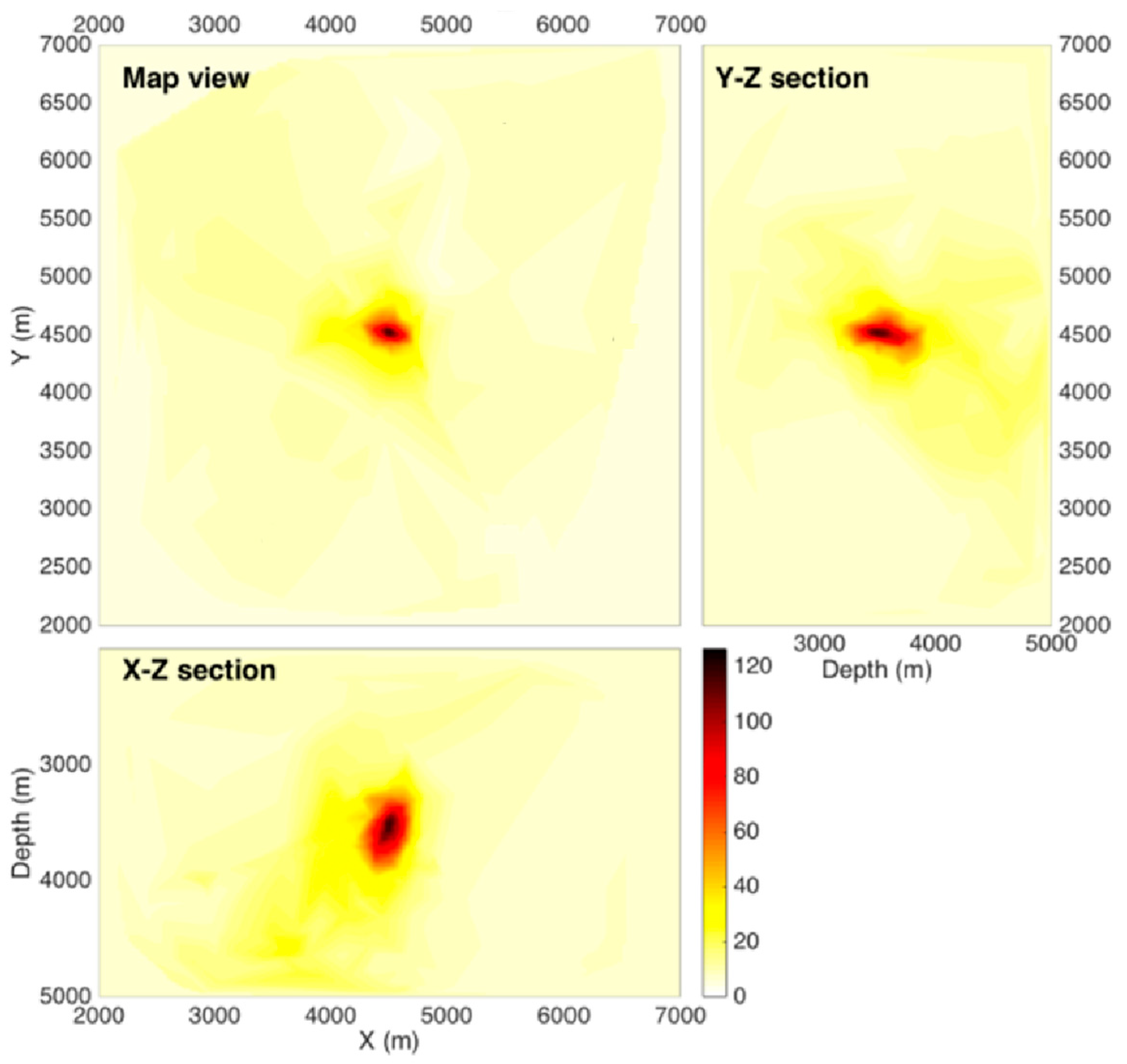
Figure A1.
Beamforming energy stacking map for event location.
Figure A1.
Beamforming energy stacking map for event location.
Appendix B
Table A1.
Detailed catalogue of 35 microseismic events recorded at the No. 2 UGS facility from March to April 2024.
Table A1.
Detailed catalogue of 35 microseismic events recorded at the No. 2 UGS facility from March to April 2024.
| Event ID | Date | Time | North | East | Depth (m) | Magnitude | Location Error (m) |
|---|
| 1 | 15 March 2024 | 21:02:01 | 1270.32 | 1258 | 4047.75 | −2.05 | 94.4 |
| 2 | 17 March 2024 | 21:41:56 | 1252.49 | 1204 | 4240.09 | −1.88 | 107.2 |
| 3 | 17 March 2024 | 23:14:46 | 1341.8 | 1049.92 | 4483.02 | −1.98 | 51.52 |
| 4 | 18 March 2024 | 4:41:07 | 1252.28 | 1328.5 | 4426.31 | −2.12 | 106.4 |
| 5 | 19 March 2024 | 7:57:33 | 1135.71 | 1285 | 4235.97 | −2.09 | 88.8 |
| 6 | 19 March 2024 | 12:11:26 | 1189.53 | 1155.04 | 4323.52 | −1.93 | 81.6 |
| 7 | 20 March 2024 | 9:53:32 | 974.45 | 1038.1 | 4135.36 | −1.85 | 45.76 |
| 8 | 20 March 2024 | 16:25:01 | 938.5 | 914.67 | 4303.37 | −2.16 | 107.2 |
| 9 | 20 March 2024 | 18:45:50 | 929.82 | 1003.18 | 4044.1 | −2.19 | 106.4 |
| 10 | 22 March 2024 | 13:25:06 | 1082.14 | 1120 | 4220.26 | −2.17 | 39.76 |
| 11 | 22 March 2024 | 22:37:38 | 992.35 | 1292.8 | 4111.56 | −2.04 | 160 |
| 12 | 23 March 2024 | 20:29:09 | 1010.29 | 1014.58 | 4150.23 | −1.86 | 108 |
| 13 | 25 March 2024 | 4:41:07 | 831.4 | 1240 | 4406.43 | −2.07 | 60.56 |
| 14 | 25 March 2024 | 7:53:32 | 1071.32 | 897.16 | 3882.96 | −2.02 | 46.4 |
| 15 | 26 March 2024 | 11:41:21 | 1252.76 | 1190.29 | 4229.1 | −1.95 | 48.16 |
| 16 | 26 March 2024 | 16:55:07 | 1118.04 | 1155.13 | 3958.96 | −2.17 | 92.8 |
| 17 | 27 March 2024 | 20:43:10 | 1082.05 | 1038.28 | 4166.4 | −1.93 | 77.44 |
| 18 | 28 March 2024 | 10:40:21 | 1252.64 | 1084.9 | 4199.92 | −2.01 | 77.76 |
| 19 | 28 March 2024 | 16:43:32 | 1127.06 | 1096.57 | 4419.98 | −1.81 | 38.88 |
| 20 | 29 March 2024 | 16:24:36 | 1521.93 | 1143.43 | 4251.34 | −1.99 | 31.04 |
| 21 | 30 March 2024 | 7:10:00 | 1010.41 | 1014.85 | 4332.69 | −2.09 | 103.2 |
| 22 | 30 March 2024 | 11:18:45 | 944.8 | 1084.93 | 4216.95 | −2.1 | 91.2 |
| 23 | 31 March 2024 | 18:37:38 | 1055.2 | 1123.75 | 4087.58 | −2.03 | 152.8 |
| 24 | 31 March 2024 | 22:46:58 | 1101.51 | 1096.66 | 4312.31 | −2.07 | 44.16 |
| 25 | 3 April 2024 | 14:01:16 | 1055.2 | 1049.71 | 4332.68 | −1.87 | 19.68 |
| 26 | 3 April 2024 | 18:03:33 | 983.47 | 964.97 | 4294.05 | −2.16 | 73.92 |
| 27 | 6 April 2024 | 5:15:56 | 1144.98 | 1073.17 | 4237.02 | −2.04 | 126.4 |
| 28 | 7 April 2024 | 3:42:23 | 1073.12 | 1178.44 | 4146.39 | −2.02 | 144.8 |
| 29 | 8 April 2024 | 12:16:15 | 831.54 | 1073.32 | 4325.13 | −2.2 | 120.8 |
| 30 | 9 April 2024 | 13:02:13 | 1046.23 | 1180 | 4283.45 | −2.07 | 67.44 |
| 31 | 10 April 2024 | 14:35:10 | 1180.68 | 731.19 | 4177.09 | −2.18 | 86.4 |
| 32 | 11 April 2024 | 15:32:33 | 1279.71 | 1166.86 | 4313.56 | −2.07 | 113.6 |
| 33 | 11 April 2024 | 17:10:00 | 916.3 | 666.67 | 4417.15 | −1.97 | 108.8 |
| 34 | 20 April 2024 | 22:31:06 | 1191.05 | 699.57 | 4018.55 | −2.07 | 116.8 |
References
- Akbari, B.; Garrison, J.; Raycheva, E.; Sansavini, G. Flexibility provision in the Swiss integrated power, hydrogen, and methane infrastructure. Energy Convers. Manag. 2024, 319, 118911. [Google Scholar] [CrossRef]
- Verliac, M.; Le Calvez, J. Microseismic monitoring for reliable CO2 injection and storage—Geophysical modeling challenges and opportunities. Lead. Edge 2021, 40, 418–423. [Google Scholar] [CrossRef]
- Zhang, J.; Fang, F.; Lin, W.; Gao, S.; Li, Y.; Li, Q.; Yang, Y. Research on injection-production capability and seepage characteristics of multi-cycle operation of underground gas storage in gas field—Case study of the Wen 23 gas storage. Energies 2020, 13, 3829. [Google Scholar] [CrossRef]
- Osieczko, K.; Gazda, A.; Malindžák, D. Factors determining the construction and location of underground gas storage facilities. Acta Montan. Slovaca 2019, 24, 234–244. [Google Scholar]
- Muhammed, N.; Haq, M.B.; Al Shehri, D.A.; Al-Ahmed, A.; Rahman, M.M.; Zaman, E.; Iglauer, S. Hydrogen storage in depleted gas reservoirs: A comprehensive review. Fuel 2023, 337, 127032. [Google Scholar] [CrossRef]
- Kumar, K.R.; Honorio, H.; Chandra, D.; Lesueur, M.; Hajibeygi, H. Comprehensive review of geomechanics of underground hydrogen storage in depleted reservoirs and salt caverns. J. Energy Storage 2023, 73, 108912. [Google Scholar] [CrossRef]
- Zeng, L.; Sarmadivaleh, M.; Saeedi, A.; Chen, Y.; Zhong, Z.; Xie, Q. Storage integrity during underground hydrogen storage in depleted gas reservoirs. Earth-Sci. Rev. 2023, 247, 104625. [Google Scholar] [CrossRef]
- Bahrami, M.; Izadi Amiri, E.; Zivar, D.; Ayatollahi, S.; Mahani, H. Challenges in the simulation of underground hydrogen storage: A review of relative permeability and hysteresis in hydrogen-water system. J. Energy Storage 2023, 73, 108886. [Google Scholar] [CrossRef]
- Gao, G.; Zhang, Y.; Yang, Z.; Duan, B.; Liu, W.; Zhang, X.; Liu, M. Sealing integrity in faulted underground gas storage: A case study of the Nanpu-1 gas storage, Eastern China. Energy Rep. 2025, 13, 1004–1013. [Google Scholar] [CrossRef]
- Carpenter, C. Integrated Approach Optimizes Underground Gas-Storage Process. J. Pet. Technol. 2023, 75, 51–54. [Google Scholar] [CrossRef]
- Ma, X. Geological Evaluation for Gas Storage Construction in Reservoirs. In Handbook of Underground Gas Storages and Technology in China; Springer: Singapore, 2021; pp. 541–574. [Google Scholar]
- Fabriol, H.; White, D.; Maxwell, S.; Deflandre, J.P.; Jousset, P. Microseismic monitoring of CO2 injection at the Weyburn oil field, Saskatchewan, Canada. In Greenhouse Gas Control Technologies 7; Elsevier Science Ltd.: Oxford, UK, 2005; pp. 2125–2129. [Google Scholar] [CrossRef]
- Mortazavi, A.; Maratov, T. An Investigation of Fault Geometric Effects on Fault Activation Mechanisms in CO2 Storage. In Proceedings of the 58th U.S. Rock Mechanics/Geomechanics Symposium, Golden, CO, USA, 23 June 2024. [Google Scholar] [CrossRef]
- Zhao, J.; Liu, P.; Li, J.; Chen, Z.; Li, Y.; Li, F. Fracture propagation induced by hydraulic fracturing using microseismic monitoring technology: Field test in CBM wells in Zhengzhuang region, Southern Qinshui Basin, China. Front. Earth Sci. 2023, 11, 1130280. [Google Scholar] [CrossRef]
- Meng, L.; Zheng, J.; Yang, R.; Peng, S.; Sun, Y.; Xie, J.; Li, D. Microseismic monitoring technology developments and prospects in CCUS Injection engineering. Energies 2023, 16, 3101. [Google Scholar] [CrossRef]
- Jahandideh, A.; Hakim-Elahi, S.; Jafarpour, B. Inference of rock flow and mechanical properties from injection-induced microseismic events during geologic CO2 storage. Int. J. Greenh. Gas Control 2021, 105, 103206. [Google Scholar] [CrossRef]
- Ry, R.V.; Septyana, T.; Widiyantoro, S.; Nugraha, A.D.; Ardjuna, A. Borehole microseismic imaging of hydraulic fracturing: A pilot study on a coal bed methane reservoir in Indonesia. J. Eng. Technol. Sci. 2019, 51, 251–271. [Google Scholar] [CrossRef]
- Qin, S.I.; Cheng, J.; Zhu, S. The application and prospect of microseismic technique in coalmine. Procedia Environ. Sci. 2012, 12, 218–224. [Google Scholar] [CrossRef]
- De Barros, L.; Guglielmi, Y.; Cappa, F.; Nussbaum, C.; Birkholzer, J. Induced microseismicity and tremor signatures illuminate different slip behaviours in a natural shale fault reactivated by a fluid pressure stimulation (Mont Terri). Geophys. J. Int. 2023, 235, 531–541. [Google Scholar] [CrossRef]
- Kraaijpoel, D.A.; Nieuwland, D.A.; Dost, B. Microseismic monitoring and subseismic fault detection in an underground gas storage. In Proceedings of the 4th EAGE Passive Seismic Workshop, Lisbon, Portugal, 17–20 March 2013; p. cp-337. [Google Scholar] [CrossRef]
- Hangx, S.J.T.; Spiers, C.J.; Peach, C.J. The effect of deformation on permeability development in anhydrite and implications for caprock integrity during geological storage of CO2. Geofluids 2010, 10, 369–387. [Google Scholar] [CrossRef]
- Tong, Z.; Hu, Z.; Qiu, L.; Zhang, N.; Zhu, H.; Zhou, D.; Hu, J. Comprehensive geological analysis and evaluation of the feasibility of renovating the Wanshunchang gas reservoir into a gas storage facility. Sci. Rep. 2025, 15, 407. [Google Scholar] [CrossRef]
- Franceschini, A.; Zoccarato, C.; Baldan, S.; Frigo, M.; Ferronato, M.; Janna, C.; Isotton, G.; Teatini, P. Unexpected fault activation in underground gas storage. Part I: Mathematical model and mechanisms. arXiv 2023, arXiv:2308.02198. [Google Scholar] [CrossRef]
- Zhang, G.; Zhu, S.; Zeng, D.; Jia, Y.; Mi, L.; Yang, X.; Zhang, J. Sealing capacity evaluation of underground gas storage under intricate geological conditions. Energy Geosci. 2024, 5, 100292. [Google Scholar] [CrossRef]
- Zhang, Y.; Shang, L.; Wang, M. Tectonic stability of the Nanpu sag: Evidence from temporal and spatial characteristics of seismic activity. J. Geomech. 2025, 31, 313–324. [Google Scholar] [CrossRef]
- Gao, G.; Ma, L.; Wu, Y.; Chen, J.; Wang, J. Geological characteristics of sandy debris flow reservoir in PG2 Block of Nanpu Sag. Fault-Block Oil Gas Field 2018, 25, 11–15. [Google Scholar] [CrossRef]
- Liu, X.; Zhang, C. Nanpu sag of the Bohai Bay basin: A transtensional fault-termination basin. J. Earth Sci. 2011, 22, 755–767. [Google Scholar] [CrossRef]
- Zhu, W.; Beroza, G.C. PhaseNet: A deep-neural-network-based seismic arrival-time picking method. Geophys. J. Int. 2019, 216, 261–273. [Google Scholar] [CrossRef]
- Mousavi, S.M.; Ellsworth, W.L.; Zhu, W.; Chuang, L.Y.; Beroza, G.C. Earthquake Transformer—An attentive deep-learning model for simultaneous earthquake detection and phase picking. Nat. Commun. 2020, 11, 3952. [Google Scholar] [CrossRef] [PubMed]
- King, A.; Talebi, S. Anisotropy effects on microseismic event location. Pure Appl. Geophys. 2007, 164, 2141–2156. [Google Scholar] [CrossRef]
- Yu, C.P.; Shapiro, S.A. Rock physics constrained estimation of shale anisotropy for microseismic processing—From VTI to orthorhombic. In Proceedings of the 77th EAGE Conference and Exhibition, Madrid, Spain, 1–4 June 2015; Volume 2015, pp. 1–5. [Google Scholar] [CrossRef]
- Zhang, Y.; Eisner, L.; Barker, W.; Mueller, M.C.; Smith, K.L. Effective anisotropic velocity model from surface monitoring of microseismic events. Geophys. Prospect. 2013, 61, 919–930. [Google Scholar] [CrossRef]
- Fomel, S. On anelliptic approximations for qP velocities in VTI media. Geophys. Prospect. 2004, 52, 247–259. [Google Scholar] [CrossRef]
- Allen, R.V. Automatic earthquake recognition and timing from single traces. Bull. Seismol. Soc. Am. 1978, 68, 1521–1532. [Google Scholar] [CrossRef]
Figure 1.
Key challenges in converting reservoirs to underground gas storage.
Figure 1.
Key challenges in converting reservoirs to underground gas storage.
Figure 2.
Integrated layout of microseismic observation stations and geological background at the No. 2 UGS facility in the Jidong Oilfield. Yellow and red triangles represent surface and shallow borehole geophone stations, respectively. The background image is a satellite photograph with overlaid structural faults (black lines), color-coded reservoir boundaries, geographic coordinates, and a location inset showing the regional context within northern China.
Figure 3.
Field deployment of seismic stations: (a) Surface station: a three-component geophone installed using shallow burial in unconsolidated soil, with manual excavation and backfilling. (b) Borehole station: deployment of a downhole geophone array into a pre-existing well, using steel cables and mechanical winches. (c) Mobile interface: real-time transmission and visualization of seismic waveform data via a mobile application.
Figure 4.
One-dimensional layered velocity model with three lithological units: upper caprock (0–2000 m), lower caprock (2000–3000 m), and reservoir (3000–4500 m). Colored backgrounds denote stratigraphic zones; black dashed lines indicate major geological boundaries. Velocity profiles are based on well logging data.
Figure 5.
(a) Frequency and maximum magnitude of recorded microseismic events; (b) injection volume and wellhead pressure profiles for wells 3634 and 3804; (c) injection volume and wellhead pressure profiles for wells 3802 and QK1.
Figure 5.
(a) Frequency and maximum magnitude of recorded microseismic events; (b) injection volume and wellhead pressure profiles for wells 3634 and 3804; (c) injection volume and wellhead pressure profiles for wells 3802 and QK1.
Figure 6.
Raw microseismic waveforms recorded for the concealed event on 8 April 2024.
Figure 6.
Raw microseismic waveforms recorded for the concealed event on 8 April 2024.
Figure 7.
Three-component spectrum analysis of Station 01 recorded in the Eastern Hebei Region on 8 April 2024, showing time-domain signals, FFT spectra, power spectral densities (PSD), and spectrograms for the east–west, north–south, and vertical components.
Figure 7.
Three-component spectrum analysis of Station 01 recorded in the Eastern Hebei Region on 8 April 2024, showing time-domain signals, FFT spectra, power spectral densities (PSD), and spectrograms for the east–west, north–south, and vertical components.
Figure 8.
(a) Daily microseismic event frequency and maximum magnitude; (b) statistical distribution of event location errors.
Figure 8.
(a) Daily microseismic event frequency and maximum magnitude; (b) statistical distribution of event location errors.
Figure 9.
(a) Depth distribution histogram of microseismic events, with colored zones representing the injection intervals of four wells; (b) well trajectories and spatial distribution of microseismic events.
Figure 9.
(a) Depth distribution histogram of microseismic events, with colored zones representing the injection intervals of four wells; (b) well trajectories and spatial distribution of microseismic events.
Table 1.
Specifications of surface and shallow borehole geophones deployed at the UGS site.
Table 1.
Specifications of surface and shallow borehole geophones deployed at the UGS site.
| Parameter | Surface Nodal Geophone | Shallow Borehole Geophone |
|---|
| Model | WF-Node3C | Custom Three-Component Geophone |
| Manufacturer | Hefei Guowai IoT Technology Co., Ltd. | Weihai Shuangfeng Geophysical Equipment Co., Ltd. |
| Place of Manufacture | Hefei, China | Weihai, China |
| Natural Frequency | 4.5 Hz | 2 Hz ±15% |
| Harmonic Distortion | <1% | ≤0.3% |
| Sensitivity | 190 V/m/s | 260 V/m/s ±15% |
| Disclaimer/Publisher’s Note: The statements, opinions and data contained in all publications are solely those of the individual author(s) and contributor(s) and not of MDPI and/or the editor(s). MDPI and/or the editor(s) disclaim responsibility for any injury to people or property resulting from any ideas, methods, instructions or products referred to in the content. |
© 2025 by the authors. Licensee MDPI, Basel, Switzerland. This article is an open access article distributed under the terms and conditions of the Creative Commons Attribution (CC BY) license (https://creativecommons.org/licenses/by/4.0/).


 ,
, 
