Wind Power Short-Term Prediction Method Based on Time-Domain Dual-Channel Adaptive Learning Model

Abstract

Driven by dual carbon targets, the scale of wind power integration has surged dramatically. However, its strong volatility causes insufficient short-term prediction accuracy, severely constraining grid security and economic dispatch. To address three key challenges in extracting temporal characteristics of strong volatility, adaptive fusion of multi-source features, and enhancing model interpretability, this paper proposes a Time-Domain Dual-Channel Adaptive Learning Model (TDDCALM). The model employs dual-channel feature decoupling: one Transformer encoder layer captures global dependencies while the raw state layer preserves local temporal features. After TCN-based feature compression, an adaptive weighted early fusion mechanism dynamically optimizes channel weights. The ACON adaptive activation function autonomously learns optimal activation patterns, with fused features visualized through visualization techniques. Validation on two wind farm datasets (A/B) demonstrates that the proposed method reduces RMSE by at least 8.89% compared to the best deep learning baseline, exhibits low sensitivity to time window sizes, and establishes a novel paradigm for forecasting highly volatile renewable energy power.

1. Introduction

Under the carbon neutrality target, the rapid growth of integrated wind power intensifies grid stability challenges caused by wind energy’s inherent intermittency. Wind power prediction, as a key link in new energy dispatch and stable operation of the power grid, has received widespread attention in recent years. Accurate wind power prediction not only helps improve the operational efficiency of the power system, but also enhances the grid’s ability to accept fluctuating power sources, thereby promoting the effective utilization and integration of wind energy. In this context, it is particularly important to study efficient wind power prediction methods.

The forecasting tasks for wind power can be divided into three categories based on time scale: ultra short term (minute level), short term (hour level), and regional day ahead forecasting. Among them, ultra-short-term forecasting focuses on real-time processing of high-frequency data, while short-term forecasting requires a balance between accuracy and computational efficiency. Current research on ultra-short-term and short-term wind power forecasting has continued to deepen in aspects such as model improvement and combination, feature extraction, and interpretability. Regarding predictive model applications, early research relied heavily on statistical models (such as autoRegressive integrated moving average (ARIMA), support vector machine (SVM)), or traditional machine learning (such as artificial neural network (ANN)), but was limited by its ability to model volatility, randomness, and complex nonlinear relationships, making it difficult to meet high-precision requirements [1]. With the rise of deep learning technology, models based on long short-term memory model (LSTM), gated recurrent unit (GRU), temporal convolutional network (TCN), Transformer, etc., have become mainstream due to their strong ability to capture temporal features. However, single models still have insufficient generalization ability in complex meteorological scenarios, prompting researchers to turn to hybrid models. For example, reference [2] combines wave division (WD), improved gray wolf optimizer based on fuzzy C-means clusters (IGFCM), and Seq2Seq model with attention mechanism based on LSTM to propose a new short-term wind power prediction method. However, RNNs like LSTM and GRU cannot parallelize computations due to sequential time-step processing, leading to slower computational speed. Their hidden state transmission mechanisms also suffer from gradient vanishing/exploding when modeling long-term dependencies. Reference [3] designed a multitask learning framework called multi-task temporal feature attention—LSTM (MTTFA-LSTM) that integrates attention mechanisms to enhance multivariate prediction capabilities. However, standalone attention layers only perform single global interaction on input sequences, lacking the hierarchical information refinement of Transformer encoders (shallow layers capture local patterns; deep layers integrate complex semantics), resulting in insufficient feature representation depth. A convolutional neural network—bidirectional LSTM (CNN-BiLSTM) model was constructed by combining multi-head attention mechanism in reference [4], which captures long-term dependencies in wind power time series through global feature extraction. While multi-head attention improves representation ability by parallelizing multiple attention heads to capture diverse interaction patterns, it remains purely linear operations without stabilization mechanisms for deep stacking. Additionally, Reference [5] combines CNN and LSTM to extract spatiotemporal features, and reference [6] proposes a novel hybrid structure for wind power interval prediction based on predicted density estimation. Reference [7] proposed an adaptive weighted combination prediction method based on deep deterministic policy gradient (DDPG) to consider local behavior accompanied by external environmental changes. Reference [8] used ensemble learning methods to combine preprocessing methods, empirical mode decomposition (EMD), information-based methods, permutation entropy (PE), and machine learning techniques (artificial neural networks, ANNs) to achieve stronger wind power prediction performance than a single ANN. Reference [9] proposed a new neural network-based ensemble system for predicting wind speed.

In addition, the quality of feature extraction directly impacts predictive performance. Current research optimizes input features through strategies such as multi-source data fusion, feature selection and denoising, and decomposition techniques. In terms of multi-source data fusion, reference [10] integrates meteorological data (wind speed, wind direction, temperature, pressure), geographic information (wind field layout), and historical power data. Reference [11] proposed a cross regional data transfer learning framework (WG Refine), but its adaptability to complex terrain areas still needs to be validated. In terms of feature selection and denoising, reference [1] adopts a hybrid adaptive decomposition denoising algorithm to solve the problems of unreasonable decomposition and residual noise. In terms of decomposition techniques, methods such as variational mode decomposition (VMD) and empirical mode decomposition (EMD) are widely used in multi-scale analysis. Reference [12] combines VMD and GRU to achieve accurate wind power prediction, while reference [7] decomposes subsequences into VMD and inputs them into ANN. Meanwhile, references [4,13] used the multivariate variational mode decomposition (MVMD) method to simultaneously analyze wind power and meteorological sequences. Reference [14] uses the Energy Entropy Theory (EVMD) to determine the number of VMD and solve the problem of excessive VMD. Reference [15] proposes a VMD-CEMDAN dual decomposition strategy to improve model prediction accuracy. The quadratic decomposition ensemble BiLSTM model in reference [4] reduces noise interference through multi-level decomposition. The aforementioned studies have not adequately considered the incomplete feature extraction at individual time steps from a local-global perspective, nor have they sufficiently explored how to improve accuracy through this approach.

In addition, in terms of model interpretability, existing research has gradually introduced feature analysis and visualization methods. Reference [16] combines the SHAP (Shapley Additive exPlans) algorithm to quantify the importance of features and clarify the impact of key variables such as wind speed and temperature on prediction results; reference [17] proposed the IFTT model, which utilizes Variable Attention Network (VAN) and Decoupled Feature Temporal Self Attention Network (DFTA) modules to enhance interpretability and provide a basis for decision support. However, most deep learning models still face the “black box” problem and urgently need to develop interpretable frameworks (such as attention visualization) to provide transparent explanations for the decision-making process. Although the inertia seal optimization algorithm (ISOA) in reference [1] improves model robustness by dynamically adjusting parameters, the physical meaning analysis of providing weight allocation is not yet complete. In addition, although the Graph Attention Network (GAT) in reference [18] can model the spatial correlation of wind fields, its graph structure construction process relies heavily on manual experience and urgently needs to be combined with automated graph learning methods (such as GraphSAGE) to improve interpretability. Current interpretability methods predominantly rely on post hoc interpretation tools, neglecting intuitive visualization of latent regularities within the features actually extracted by models.

In summary, three critical research gaps persist:

(1)

Feature Decoupling Deficiency: While extensive exploration has been conducted on hybrid models in wind power forecasting, few architectures systematically integrate the global dependency modeling advantages of Transformers with the local feature extraction capabilities of Temporal Convolutional Networks (TCNs). This separation prevents synergistic interaction between two critical features: on one hand, Transformers can model long-term dependencies across time steps but may lose local fluctuation details and native sequential characteristics due to positional encoding mechanisms; on the other hand, TCNs excel at capturing sequential order and local features but exhibit weaker global feature extraction due to limited receptive fields. This fragmentation creates a “global-local imbalance” dilemma in complex wind power scenarios—prediction accuracy remains improvable when handling highly volatile sequences.

(2)

Dynamic Adaptation Gap: Mainstream hybrid models depend on static fusion strategies (e.g., simple concatenation or fixed-weight summation), failing to adapt to dynamically evolving wind power fluctuation patterns. Meanwhile, adaptive activation function properties are often overlooked. Breaking through these rigid mechanisms can enhance deep learning models’ adaptive feature fusion capabilities, further improving training quality and predictive accuracy.

(3)

Interpretability Barrier: Existing studies face “interpretability fragmentation” issues. Traditional methods either ignore self-interpretability exploration or depend on post hoc tools, seldom focusing on the latent regularity expressions of extracted features themselves. This hinders deeper understanding of how deep learning models comprehend features.

To bridge the aforementioned research gaps, this study makes the following contributions:

(1)

Feature Decoupling-Fusion Paradigm: Addressing the “global-local imbalance”, we propose a dual-channel temporal learning architecture that innovatively integrates Transformer’s global dependency modeling with TCN’s local feature extraction. This hybrid framework combines series-parallel configurations to preserve original sequence characteristics lost during Transformer encoding. The global channel employs Transformer encoder to capture long-term temporal evolution patterns, while the local channel utilizes dilated convolution TCN residual blocks to precisely extract localized abrupt features after linear transformation. Prior to model training, we apply the Isolation Forest algorithm [19] for unsupervised outlier detection in wind power data, exploring internal two-dimensional patterns and eliminating anomalies.

(2)

Dual-Level Adaptive Learning Mechanism: We introduce dynamic optimization at both feature fusion and activation function levels. For feature fusion, we replace static weights with learnable parameters through differentiable channel weighting optimization. The architecture integrates ACON adaptive activation functions to enhance dynamic regulation capabilities during training, breaking through conventional deep learning models’ adaptability limitations.

(3)

Interpretable Feature Visualization: We visualize adaptively fused features through scatter/kde plots, demonstrating the model’s intrinsic understanding of wind power characteristics. This visualization facilitates interpretation of how deep learning models comprehend temporal features through our dual-channel extraction and adaptive fusion processes.

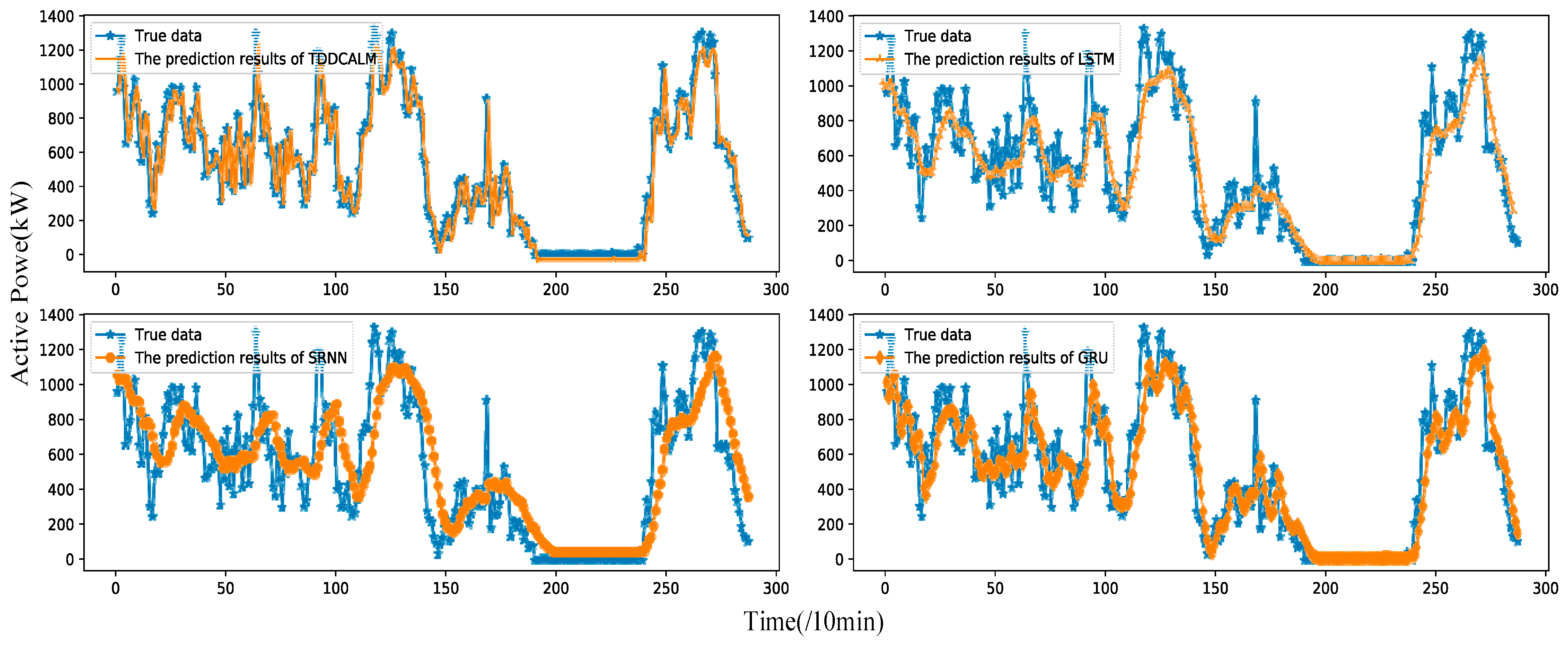
To verify the reliability of the proposed method using actual wind power datasets, comparisons with traditional models showed that this method can effectively extract the characteristics of severe fluctuations in time-domain signals, and the prediction results are sufficient to meet the accuracy requirements of short-term wind power prediction. Without any artificial noise reduction, it can still achieve good results.

The rest of this paper is organized as follows: Section 2 introduces the data processing workflow. Section 3 describes the basic architecture of the TDDCALM. Section 4 presents the short-term wind power prediction method based on the TDDCALM. Section 5 details the case study section. Section 6 concludes this paper.

2. Data Preprocessing

2.1. Outlier Screening

Considering the large number of uncertain factors in real engineering scenarios and the chaotic nature of weather and other systems, measurement results and prediction results are prone to errors. If there are a large number of outliers in the initial dataset, it can easily cause a shift in the model’s final state. Therefore, it is necessary to use reasonable anomaly detection algorithms to screen for outliers. Common anomaly detection algorithms mainly include model-based, distance-based, and density-based methods [20,21,22]. The main operation is to describe normal samples and characterize their regions in the feature space, while treating samples outside the region as anomalies [23]. This type of method has certain limitations: the anomaly detector only optimizes the description of normal samples and ignores abnormal samples, which may result in false positives or only in detecting a small number of anomalies [24].

Given the aforementioned shortcomings, this article selects the Isolation Forest algorithm to screen for outliers in the raw data. Isolation forest (IForest) adopts ensemble learning strategy and is a high-precision anomaly detection algorithm [25]. This algorithm focuses on building and fusing multiple sub detectors to achieve better detection performance and lower relative complexity. The core idea is to use hyperplanes for random cyclic segmentation of continuous data, search for data points with shorter paths, that is, isolated points with sparse distribution and far distance from high-density populations, and classify them as outliers. Clusters with higher density often require multiple partitions to isolate, while outliers with lower density require the opposite. The data applicable to this algorithm should include the following two features:

(1)

The proportion of abnormal data to the total sample is relatively small;

(2)

There is a significant difference between the characteristic values of outliers and normal points.

The collection of wind power raw data by this research institute can simultaneously meet the above two requirements. A parallel dataset of power wind speed is constructed, considering the coupling relationship between wind power and wind speed. Within the feature space formed by the two, the dataset is randomly segmented using an isolated forest, isolated points are screened, and the model detection capability is optimized to ultimately complete the screening of outliers in wind power time series data.

Given d-dimensional feature sample data X = {x₁, ……, x_n}, attribute q and partition value p are randomly selected to cyclically partition the samples, while increasing the tree height. When the following three conditions are met during the process, the partitioning is stopped:

(1)

The tree height has reached its limit;

(2)

When |X| = 1;

(3)

All data values in sample X are the same.

Assuming that all sample elements x are different, when the isolated tree grows completely, each instance is isolated to an external node, where the number of external nodes is n and the number of internal nodes is (n − 1). The anomaly score S (x, n) of instance x is now defined as Equation (1).

$$S(x,n)=2^{-{\displaystyle \frac{E(h(x))}{c(n)}}}$$

(1)

$$c(n)=2H(n-1)-(2(n-1)/n)$$

(2)

where h(x) is the sample path, E(h(x)) is the expected path length of sample x in a group of isolated trees, and c(n) in Equation (2) is the average path length of search failures in BST.

Regarding the method of detecting abnormal samples, reference [21] provides relevant criteria:

(1)

If the sample returns an S value very close to 1, it can be classified as an abnormal sample;

(2)

If S is much smaller than 0.5, it can be considered a normal instance;

(3)

If all samples return S ≈ 0.5, then the sample as a whole has no significant abnormalities.

The algorithm classifies the data within the decision boundary as normal values, while treating the data outside as abnormal. At the same time, it separates the two and processes them into experimentally usable data.

Divide the data into three intervals based on the distribution of wind speed: high wind speed zone, medium wind speed zone, and low wind speed zone. Construct three types of wind speed wind power parallel data and use isolated forests for unsupervised training and detection of outliers.

2.2. Standardization

To improve the fitting accuracy of the model to the data and achieve better convergence effect of gradient descent, it is necessary to process the data into a reasonable data state. The Transformer encoder and TCN are sensitive to feature scaling, so this paper adopts the Min–Max method to normalize the model, scaling the features to between [0, 1], as shown in Equation (3).

$$x^{\prime }={\displaystyle \frac{x-Min(x)}{Max(x)-Min(x)}}$$

(3)

where x is the original data point, and x’ is the normalized state of the data. Min(x) represents the minimum value of the sequence, and Max(x) represents the maximum value of the sequence. The sequences used in subsequent experiments in this article are all composed of x′.

3. Architecture of TDDCALM

Transformer performs excellently in sequence modeling tasks due to its parallelizability, non-strict data requirements, and many superiorities, making it widely used in sequence generation tasks. When processing time series data, Transformer relies entirely on attention mechanisms, which can avoid long-range dependency problems and effectively mine global features of the sequence. However, for time series with high volatility, Transformer often performs slightly worse. In addition, this article believes that the position encoding method may result in the loss of some sequence features.

Besides Transformer, TCN, as one of the commonly used models for time series modeling, has more stable gradients and smaller memory than RNNs. Structurally, residual connection blocks [26] are advantageous for training deep TCN architectures, dilated convolutions provide flexible receptive fields, and causal convolutions [27] can rely solely on past data for data extraction, without the problem of leakage of future data to be predicted. The above structural characteristics enable it to exhibit performance close to or even surpassing RNNs in most time series modeling and regression prediction tasks. TCN has obvious advantages, but due to its limited receptive field, it is not suitable for problems that require long-term memory, and it is difficult to achieve the effect of extracting global features in a single turn with Transformer. This article combines the advantages of both and proposes a modeling method that integrates two different data features.

Firstly, decouple the data into different channels and divide them into the following two forms:

(1)

Feature vectors encoded by Transformer;

(2)

Linear transformation layer of raw data.

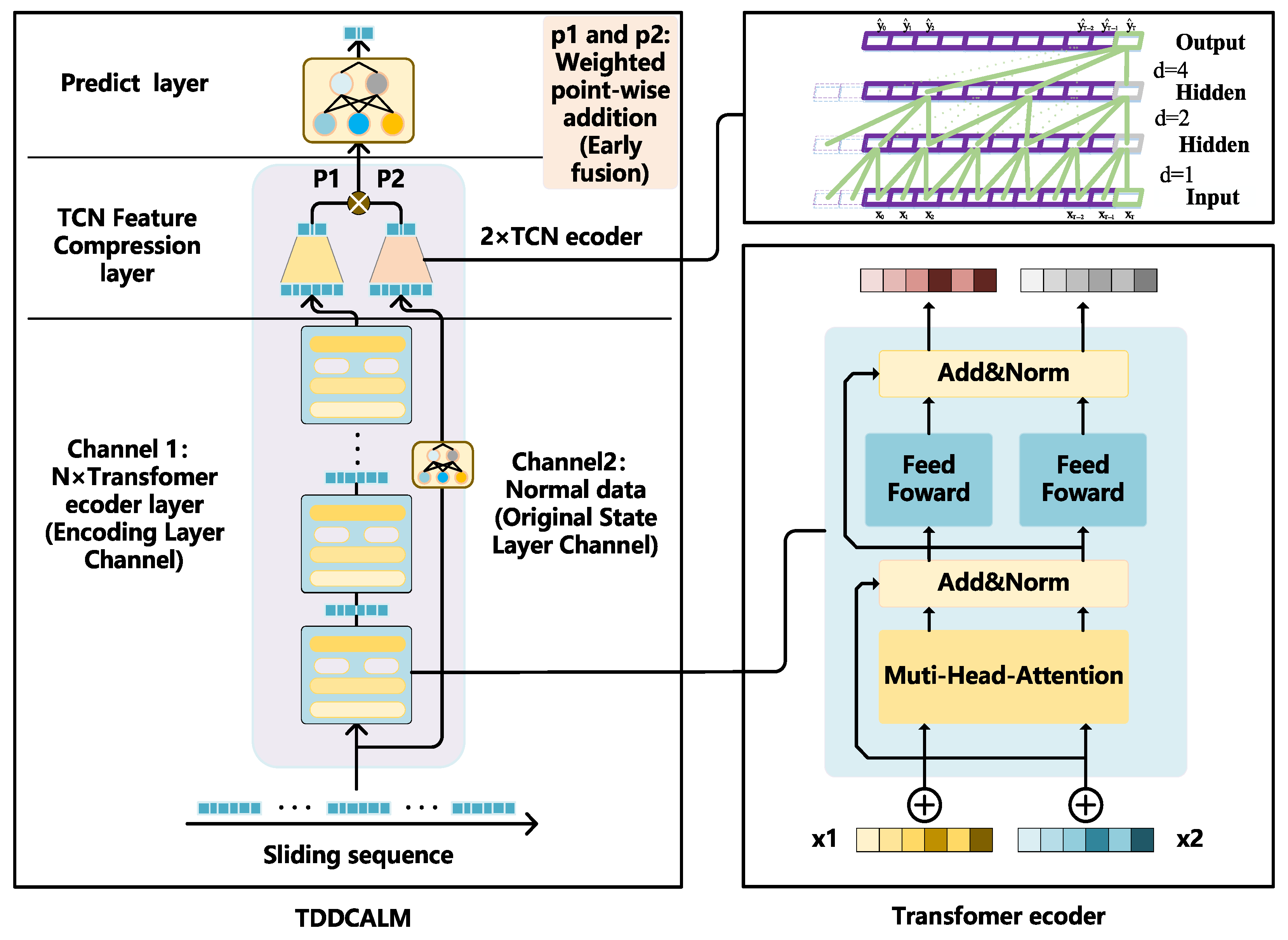
Perform feature extraction on the above two channels separately. Channel 1 integrates attention mechanism and contains global dependency information of input sequence elements. The output data has discreteness, and although there is positional encoding to represent element positions, some sequential features may still be missing. Channel 2 possesses the sequential features missing from channel 1, but cannot represent the global dependencies of individual elements. The emphasis of the two is different, and this article believes that the above two features should be involved in training simultaneously. Based on the above ideas, this article proposes the TDDCALM. TDDCALM feeds channel 1 and channel 2 into two TCN encoders for feature compression, and performs adaptive weighted early fusion on the compressed features. In Channel 2, the primary purpose of applying a linear transformation layer to raw data is to extract and enhance useful features. Although these features originate from the original data, linear transformation enables more effective identification of underlying patterns or relationships within the data structure. This operation improves learning efficiency and representation quality in subsequent TCN layers. Furthermore, linear transformation facilitates partial normalization of data distribution discrepancies, thereby enhancing model generalization capabilities. Simultaneously add ACON adaptive activation function layer instead of ReLU. The depth of the model helps to obtain more complex temporal fluctuation characteristics, while the width of the model (i.e., two channels) enables the TDDCALM to use an adaptive weighted early fusion mechanism to allocate channel weights reasonably, thereby adapting to sequence prediction tasks with different fluctuation characteristics. The basic structure of the TDDCALM is shown in Figure 1, which may be more concise compared to Transformer:

3.1. Original State and Encoding Layer Channel

Reference [28] proposed a temporal representation learning framework based on a Transformer encoder, which does not use a decoder and only utilizes the encoder for unsupervised representation learning of the temporal sequence. The obtained feature vectors can be applied to downstream tasks such as regression and classification with good results. Only using an encoder structure can reduce the training parameters by half while ensuring the effectiveness of feature extraction. This article draws on this idea and uses a Transformer encoder to perform the first feature encoding on the temporal sequence, in order to explore the global features within the temporal sliding window of the temporal sequence. The joint training of encoding channels and predictors does not require greedy pre-training. As shown in Figure 1, channel 2 retains the serialization features of the original data, while channel 1 is encoded to contain the global dependencies of elements.

The encoding channel is composed of a serial Transformer encoder, which is mainly composed of multi-head self-attention and feedforward network. Each encoder is independent of the others and has no parameter sharing.

For input sequences H = [w₁, …, w_n] at different time steps, self-attention is applied for encoding. The attention mechanism emulates the biological process of observation, which aligns internal experiences with external sensory inputs to enhance the precision of observations in specific regions [29]. This mechanism can rapidly extract important features from sparse data through a top-down information selection process that filters out irrelevant information [30].

The self-attention mechanism improves upon the standard attention by reducing external information dependency, and is better suited for uncovering internal correlations within data and features [28], as shown in Equation (4).

$$\mathrm{Self}\text{-}\mathrm{Attention}\left(Q,K,V\right)=\mathrm{Softmax}\left({\displaystyle \frac{K^{{\rm T}}Q}{\sqrt{d_k}}}\right)V$$

(4)

$$Q=W_{Q}H, K=W_{K}H, V=W_{V}H$$

(5)

where d_k denotes the dimension of column vectors in input matrices Q and K. The projection matrices W_Q ∈ R^dk×dh, W_K ∈ R^dk×dh, and W_V ∈ R^dk×dh represent weights.

Compared to single-head attention, multi-head attention enables parameter matrices to form multiple subspaces, allowing the model to simultaneously extract information from different projection spaces. This enhances learning effectiveness and facilitates parallel training. To maximize the extraction of interaction information, the model employs multi-head self-attention, as defined in Equation (6):

$$\mathrm{Multi}\text{-}\mathrm{Head}(H)=W_O[{\mathrm{h}}_1,\dots ,{\mathrm{h}}_M]$$

(6)

$${\mathrm{h}}_m= \mathrm{SelfAtt}(Q_m, K_m, V_m)$$

(7)

$$\begin{array}{c}{Q}_m=W_Q^{m}H, K=W_K^{m}H,\\ V=W_V^{m}H\end{array}$$

(8)

In Equation (6) the output projection matrix W_O ∈ R_dh × M_dv, and projection matrices W_Qm ∈ R^dk×dh, W_Km ∈ R^dk×dh, and W_Vm ∈ R^dk×dh, where m ∈ {1, …, M}.

Traditional Transformers employ multi-head self-attention to encode sequences H = [w₁, …, w_n], but neglect positional information of sequence elements. This issue is addressed through positional encoding, with the encoded results shown in Equation (9):

$$U^{(0)}=\left[S_{w1}+P{E}_1,\dots ,S_{wN}+P{E}_N\right]$$

(9)

$$P{E}_{n,2i}=\sin \left(n/{10000}^{2i/d}\right)$$

(10)

$$P{E}_{n,2i+1}=\cos \left(n/{10000}^{2i/d}\right)$$

(11)

The embedded vector representation of a sequence element is denoted as S_wn, the vector representation at position n corresponds to its positional encoding PE_n, and the 2i dimension of the positional encoding vector at position n is denoted as PE_n,2i, where the encoding vector dimension is represented as d.

Since the sequential features lost in Transformer encoder can be compensated by another channel, this study does not implement a positional encoding mechanism here.

3.2. Tcn Feature Compression Layer

After the TDDCALM extracts information through channel division, the extracted features need to be encoded separately via two TCN structures to reduce data dimensions and condense them into more distinct features.

TCN is a fully convolutional network architecture specifically designed for sequential data, characterized by three key components:

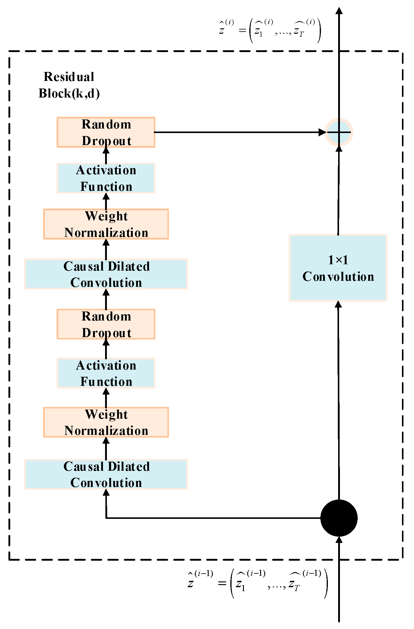
3.2.1. Residual Connections

To enable cross-layer information transmission in the network, TCN adopts residual connection patterns. As shown in Figure 2, replacing single-layer convolutions with residual block structures enhances trainability.

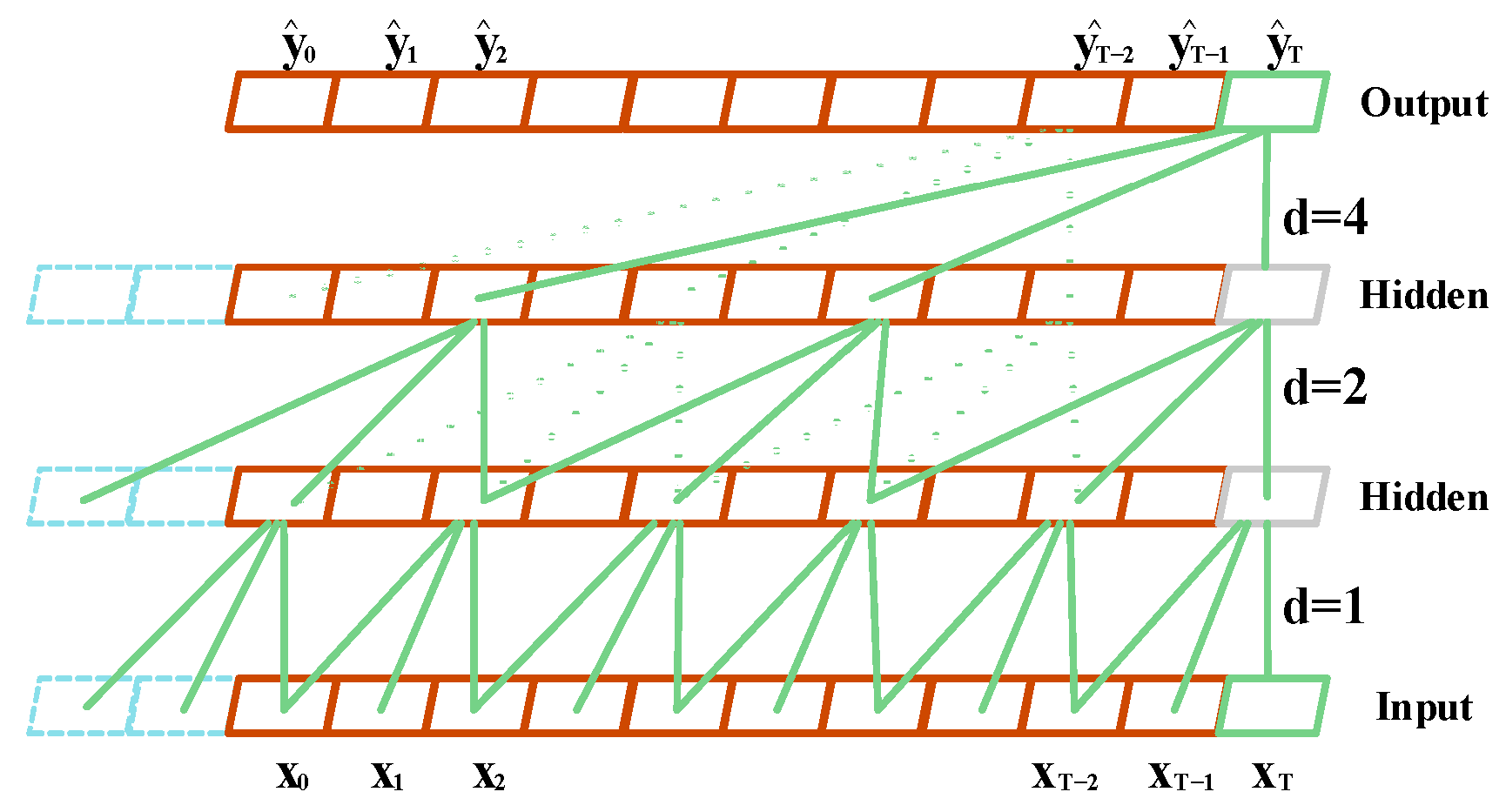
3.2.2. Dilated Convolutions

To address the problem of network depth limitations caused by fixed kernel sizes, TCN introduces dilated convolutions (also known as atrous convolutions). Unlike traditional convolutions, dilated convolutions perform sampling with interval d (as illustrated in Figure 3), which expands receptive fields across network layers, enabling flexible receptive field adaptation.

3.2.3. Causal Convolutions

To apply traditional convolutional architectures to sequential data, temporal constraints must be added through causal convolutions. This unidirectional structure only accesses past information, preventing future data leakage.

Deep neural networks benefit from residual blocks through convolutional operations and network regularization. This structure mitigates challenges associated with increasing network depth, including computational resource consumption, overfitting, gradient explosion, and vanishing gradients.

The operations of dilated convolutions and residual blocks are mathematically defined in Equations (12) and (13), respectively.

$$F\left(s\right)=\left(x{\ast }_{d}f\right)\left(s\right)={\displaystyle \sum _{i=0}^{k-1}f\left(i\right)\cdot x_{s-d\cdot i}}$$

(12)

$$o=\mathrm{Activation}\left(x+F\left(x\right)\right)$$

(13)

Here, the input is x ∈ Rⁿ, the convolution kernel is f: {0, …, k − 1}→R, and Activation(·) denotes the activation function.

3.3. Feature Adaptive Weighted Early Fusion

After the dual-channel features are encoded by TCN, further measures are required for feature fusion before the predictor [31], termed early fusion. Common early fusion strategies in deep learning theory include the following:

(1)

Sequential feature fusion, which directly concatenates the two features.

(2)

Parallel strategy fusion, which combines the two features into a composite vector.

The literature [32] introduces canonical correlation analysis (CCA) for feature fusion. This method transforms features by exploiting correlations between input features, producing transformed features with higher correlation than the original sets. However, it neglects the relationships between class structures within the dataset. To address this limitation, the literature [33] proposes a feature fusion method called DCA (Discriminant Correlation Analysis). This approach maximizes correlations between corresponding features in the two sets while simultaneously maximizing inter-class differences, effectively overcoming the shortcomings of CCA.

Considering architectural constraints and practical engineering requirements, this study proposes an adaptive weighted early fusion method to achieve reasonable weight allocation between the dual channels. Specifically, learnable channel weight coefficients are defined, and features are weighted and fused before prediction. During training, the channel coefficients are updated iteratively to optimize weight proportions. The two channels may have unequal importance, and their assigned weight coefficients may not be equal. Manual parameter tuning would incur unnecessary workload, so an adaptive mechanism is adopted to let the model automatically adjust dual-channel weights. The model outputs the trained weight results after completion, quantifying the relative importance of the two features.

In this study, the weight of the encoded channel is defined as P₁, and the weight of the raw data channel is defined as P₂. These weights must satisfy the relationship specified in Equation (14):

$$P_1=1-P_2$$

(14)

An increase in parameters could cause model redundancy and slow training speed. Therefore, Equation (14) is used to reduce parameters, with the objective of training being to converge P₁ and P₂ to an appropriate proportion. The weights are initialized through the creation of new parameters and updated during training alongside other learnable parameters in the neural network according to gradient variations from the loss function. Specifically, for each training batch, the model first performs forward propagation to obtain predicted outputs, then calculates the loss between predictions and ground truth labels. Subsequently, the system automatically computes gradients of the loss with respect to P₁ and P₂, and adjusts their values using optimization algorithms to minimize the overall loss function.

Define P = [P₁, P₂]^T Update using gradient descent

$$P^{(k+1)}=P^{(k)}-\eta \nabla L(P^{(k)})$$

(15)

where L(·) denotes the loss function, and $\nabla$L satisfies L-smooth. According to gradient descent convergence theory, when the learning rate η < L/2 (where L is the Lipschitz constant of the loss function), the weight sequence P^(k) converges to the global optimal solution P*.

Meanwhile, during training, the constraint function (14) compresses the search space into a one-dimensional subspace, effectively mitigating divergence risks inherent in high-dimensional optimization while enhancing training stability.

$$\mathcal{P}=\{{[p,1-p]}^T\mid p\in [0,1]\}$$

(16)

3.4. ACON Layer Adaptive Activation Function

Activation functions can enhance model nonlinearity, and their types influence network characteristics, thereby affecting training performance. This study adopts the adaptive activation function framework ACON (Activate or Not) [34], which autonomously learns activation states and automatically searches for optimal activation functions per layer. It includes three variants—ACON-A, ACON-B, and ACON-C—defined in Equations (17), (18), and (19), respectively. The general form is presented in Equation (20):

$$\mathrm{ACON}\text{-}\mathrm{A}(x)=x\cdot \sigma \left(\beta x\right)$$

(17)

$$\mathrm{ACON}\text{-}\mathrm{B}(x)=\left(1-q\right)x\cdot \sigma \left(\beta \left(1-q\right)x\right)+qx$$

(18)

$$\mathrm{ACON}\text{-}\mathrm{C}(x)=\left(q_1-q_2\right)x\cdot \sigma \left(\beta \left(q_1-q_2\right)x\right)+q_{2}x$$

(19)

$$\mathrm{ACON}(x)=({\eta }_a(x)-{\eta }_b(x))\cdot \sigma (\beta ({\eta }_a(x)-{\eta }_b(x)))+{\eta }_b(x)$$

(20)

The parameters q₁, q₂, and β are all learnable. During training, ACON approximates the optimal activation functions for each layer, thereby improving the model’s training performance ceiling.

Replacing traditional ReLU layers with ACON layers indirectly enhances model generalization. Meanwhile, ACON possesses higher gradient stability, enabling it to avoid gradient oscillation issues caused by the bimodal distribution of gradients in Swish/GELU functions.

In summary, the TDDCALM can be expressed as Equation (21)

$$\mathrm{T}(x)=\mathrm{L}(\mathrm{F}(\mathrm{TCN}(\mathrm{L}(x)),\mathrm{TCN}(\mathrm{Tra}(x))))$$

(21)

where F(·,·) denotes adaptive weighted early fusion, TCN(·) represents feature compression, Tra(·) indicates the encoding channel, and L (·) corresponds to linear transformation.

4. Short-Term Wind Power Forecasting Model Based on TDDCALM

Wind farm data are typically influenced by numerous internal and external factors, often exhibiting complex variations. Time series of wind power and wind speed, in particular, frequently display significant fluctuations within short periods.

As a major branch of machine learning, deep learning can enhance feature extraction capabilities of wind power data by increasing network depth and architectural complexity. Most existing wind power forecasting studies based on deep neural networks employ RNNs or TCNs for modeling. Traditional approaches, however, suffer limitations in predicting future peaks and troughs of wind power due to multiple influencing factors.

Accurate extraction of short-term wind power fluctuations hinges on precisely capturing the invariant periodic characteristics of wind power time series. Beyond stacking network layers, it is crucial to improve the model’s ability to fully utilize power time series data.

To maximize the utilization of short-term wind power data, the key lies in directing the model to extract diverse forms and perspectives of features from the same dataset. This study proposes three improvements to traditional models:

(1)

After screening outliers, wind power data are decoupled into distinct forms and perspectives of features within the model. These features are processed through two parallel channels, compensating for the disadvantage of limited data volume in short-term wind power forecasting while accounting for multiple potential influencing factors.

(2)

Constructing diverse forms and perspectives of features ensures adequate exposure of characteristics even with limited data volume. Each feature form carries an implicit importance weight. This study enables the model to adaptively adjust the contribution ratios of different features during training, thereby better accommodating the multi-layered nature of wind power time series.

(3)

Activation functions (e.g., Sigmoid, ReLU) interact with network weights, occasionally causing issues like gradient explosion—a fundamental challenge in deep learning. While self-adaptive weight adjustment already provides flexibility, this study further introduces adaptive activation functions. The model can automatically search and adjust the optimal activation function for each layer, mitigating the aforementioned problems to some extent.

The modeling process of the aforementioned study is shown in Figure 4.

4.1. Data Preprocessing and Parameter Settings

Wind turbine data collected in inland wind farms are often affected by uncontrollable factors and contain numerous outliers. These outliers are first screened using unsupervised methods and then normalized. The processed data serve as training input for subsequent model development.

The TDDCALM essentially solves an optimization problem using the mean squared error (MSE) loss function during training. Common optimization algorithms include Adam and SGD. Among these, Adam dynamically adjusts learning rates and updates parameters. This study selects Adam as the optimization algorithm and employs grid search to identify the optimal parameter combination. Key parameter settings include the following: one stacked Transformer encoder (N = 1), a TCN convolution kernel size of 3, a dropout rate of 0.2, and a compression layer with input dimensions [8324, 9, 1] and output dimensions [8324, 16]. The initial learning rate is set to 0.01.

4.2. Wind Power Time Series Feature Extraction

The Transformer encoder’s encoding operation combines multi-head self-attention, normalization, and residual units. The self-attention computation is defined in Equation (7), while the multi-head self-attention mechanism is detailed in Equation (6). Compared to basic self-attention, multi-head variants enable more comprehensive feature extraction. TCN is described as a hybrid network combining one-dimensional full convolution and causal convolution. Its convolutional operations reduce large samples to smaller ones, achieving dimensionality reduction and feature aggregation. Dilated convolutions and residual block computations are defined in Equations (12) and (13), respectively. The fused features incorporate global and sequential information from individual time windows, each carrying distinct weight contributions.

Define the wind power time series signal x_t as the sum of a global dependency component g_t and a local fluctuation component l_t

$$x_t=g_t+l_t+{ϵ}_t$$

(22)

where ϵ_t is the noise term.

The Hilbert space signal decomposition theorem states that non-stationary time series can be decoupled into slowly varying components g_t′ with long-range properties and transient components l_t′ with local properties [35]. The dual-channel structure inherently resembles a parallel approximation of these two components through orthogonal feature subspaces.

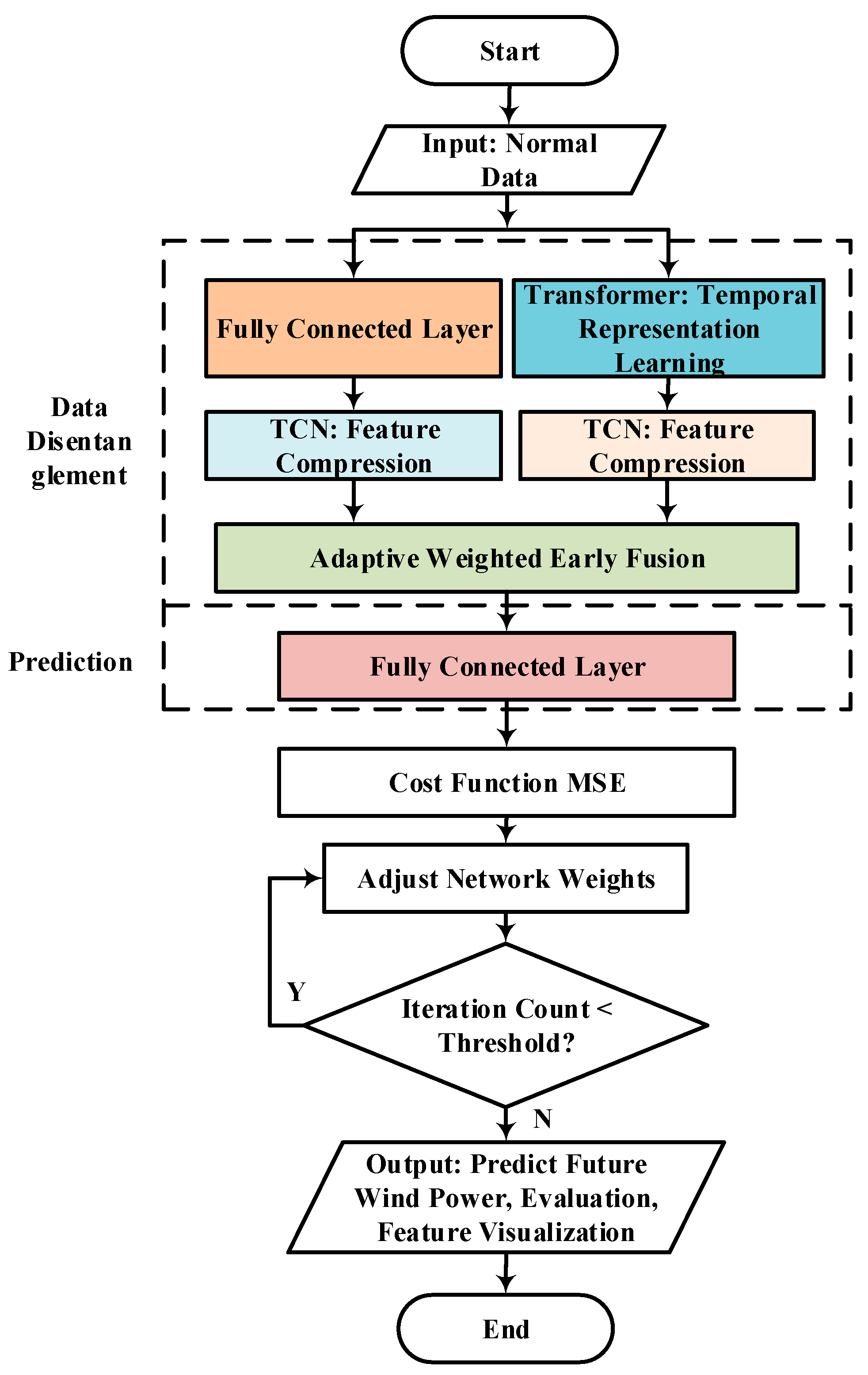
4.3. Training Process

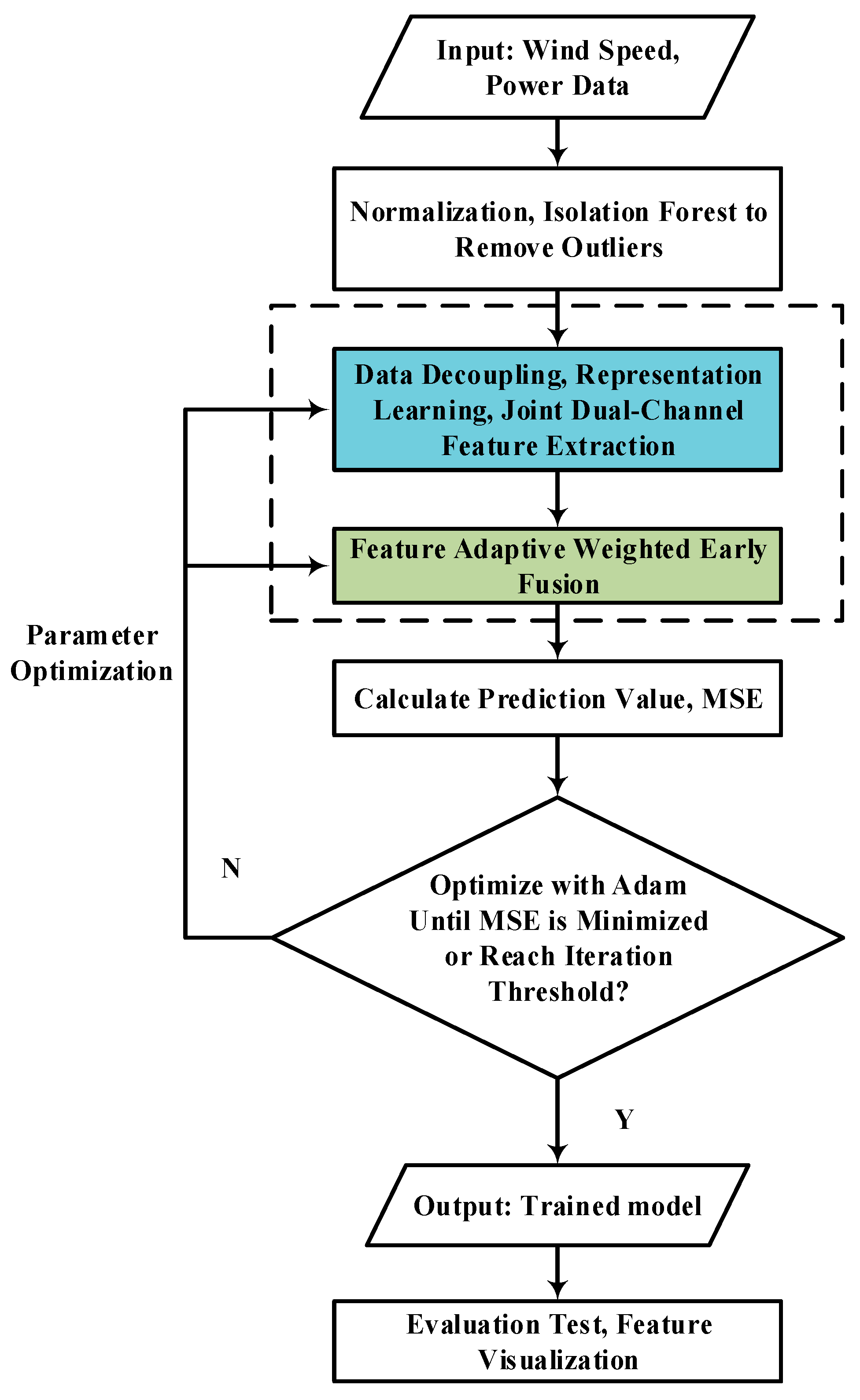
The detailed algorithm solution procedure of this study is shown in Figure 5.

As shown in Figure 5, power and wind speed are taken as inputs, normalized after outlier screening. The data is decoupled into two states, with features extracted separately from each state and then fused for training the predictor. The Adam algorithm optimizes the mean squared error (MSE), updating network weights through backpropagation according to the MSE. This process repeats until the MSE reaches its minimum value or the iteration count meets the threshold. After completion, the model outputs predicted results, fused feature latent vectors, and channel weight coefficients. The proposed model distills wind power time series into 32 key features. Subsequent sections evaluate model performance using test sets and visualize the fused features.

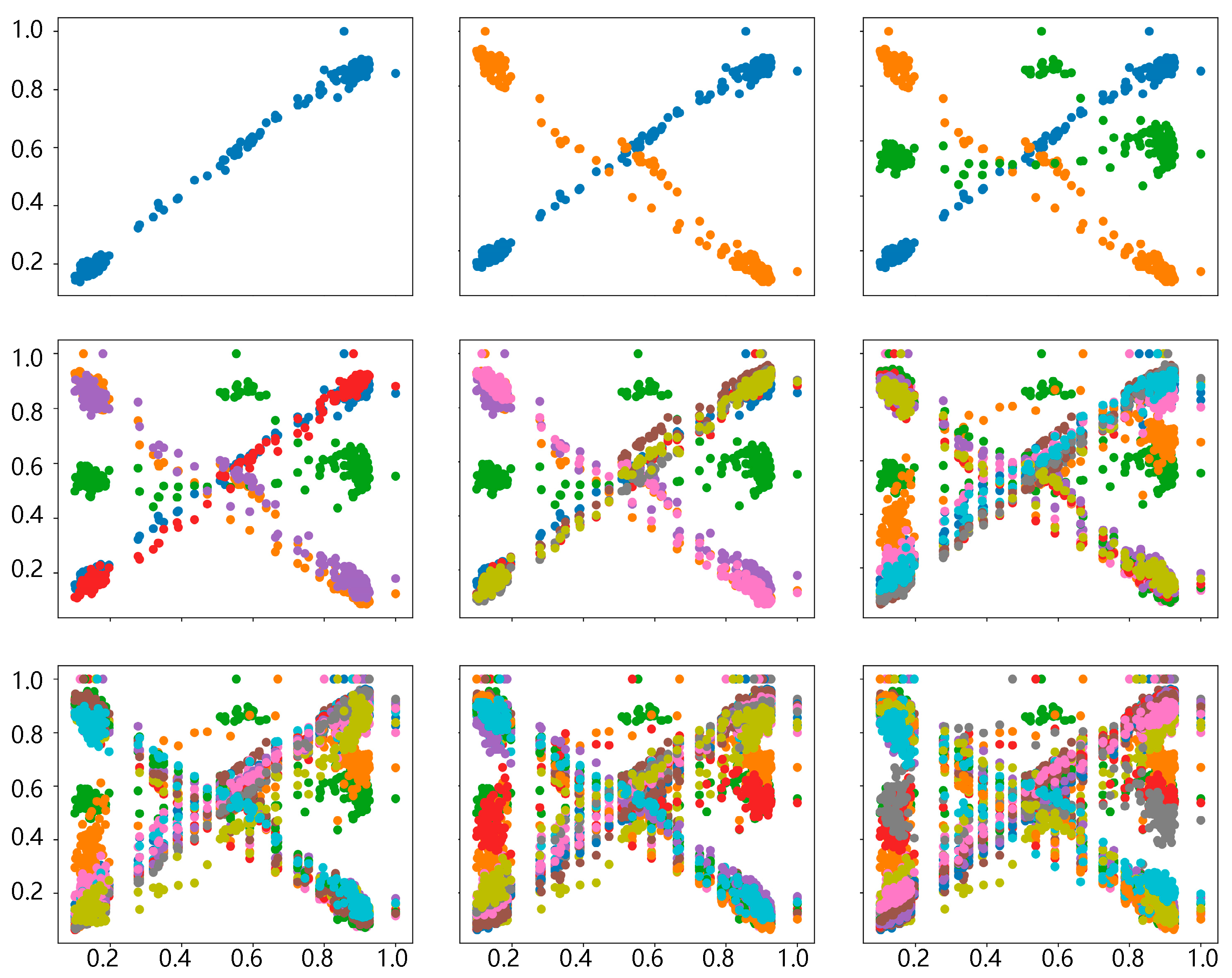
4.4. Feature Interpretation via Multiple Visualization Methods

Wind farms involve numerous internal and external influencing factors, causing complex variations in wind speed and power, particularly evident in short-term fluctuations. These characteristics are difficult to extract due to limited data volumes and multiple influencing factors.

For wind power data with multiple influencing factors, traditional methods focus on data transformation approaches, including time series signal decomposition, segmented modeling, and state processing. Post-processed modeling methods typically use shallow architectures. However, these shallow structures struggle to extract deep features from high-dimensional wind power data, which are heavily influenced by data states and types.

The proposed model employs a deep architecture capable of accurately extracting hierarchical features from wind power fluctuations. To demonstrate this explicitly, deep features are described intuitively.

Traditional feature visualization methods include heatmaps and scatter plots to show high/low-dimensional feature distributions and correlations. This paper globally samples feature vectors from the model’s base layer, presenting mapped scatter plots and inter-feature kernel density plots at the end of the document.

5. Case Study

5.1. Evaluation

To verify the accuracy of the proposed method, six common error evaluation metrics are introduced during the testing phase:

$${\epsilon }_{MSE}={\displaystyle \frac{1}{n}}{\displaystyle \sum _{i=1}^n{\left(u_{id}-{u_{id}}^{\prime }\right)}^2}$$

(23)

$${\epsilon }_{RMSE}=\sqrt{{\displaystyle \frac{1}{n}}{\displaystyle \sum _{i=1}^n{\left(u_{id}-{u_{id}}^{\prime }\right)}^2}}$$

(24)

$${\epsilon }_{MAE}={\displaystyle \frac{1}{n}}{\displaystyle \sum _{i=1}^n\left|u_{id}-{u_{id}}^{\prime }\right|}$$

(25)

$$I_{MSE}={\displaystyle \frac{1}{n}}{\displaystyle \sum _{i=1}^n{\left(v_{id}-{v_{id}}^{\prime }\right)}^2}$$

(26)

$$I_{RMSE}=\sqrt{{\displaystyle \frac{1}{n}}{\displaystyle \sum _{i=1}^n{\left(v_{id}-{v_{id}}^{\prime }\right)}^2}}$$

(27)

$$I_{MAE}={\displaystyle \frac{1}{n}}{\displaystyle \sum _{i=1}^n\left|v_{id}-{v_{id}}^{\prime }\right|}$$

(28)

Here, v_id and v_id′ represent the denormalized true and predicted values of wind power in the test set, while w_id and w_id′ denote the non-denormalized true and predicted values. The magnitudes of ε_MSE, ε_RMSE, ε_MAE, I_MSE, I_RMSE, and I_MAE characterize model prediction accuracy. Smaller values of these metrics indicate lower prediction errors.

5.2. Practical Case Study

The algorithm used in this study was implemented using Python code, with Python version 3.7. Software configurations include the PaddlePaddle 2.1.0 framework and Jupyter Notebook development environment. Hardware specifications consist of a Baidu Cloud server with GPU: Tesla V100 (Video Memory: 32 GB), CPU: 4 Cores, RAM: 32 GB, and Disk: 100 GB.

The core algorithm is applied to engineering practice to validate the effectiveness of the proposed method.

5.2.1. Prediction Error Analysis on Different Datasets

First, dataset A was constructed using power output data from wind turbine A at a certain wind farm, and dataset B was formed by the active power at the grid connection point of a small wind farm B. Wind farms A and B are located in different regions with distinct altitudes, covering both low-altitude and mountainous hill areas. To validate the generalization capability beyond wind power applications, dataset C was established using a new energy sector index from a stock market as an auxiliary validation dataset. The outlier-processed datasets (A, B, C) were strictly partitioned in chronological order into training and testing sets with different ratios to preserve temporal dependency. The test sets and training sets have no temporal overlap to prevent data leakage. Their basic information is shown in

Table 1. A, B, C dataset basic information.

Dataset	A	B	C
Source	Wind Farm A	Wind Farm B	Stock Market
Measurement	kW	kW	Index Points
Time Resolution	10 min	5 min	day
Time Span	65 d 9 h 20 min	19 d 23 h 55 min	581 days
Outliers Removed (Steps)	801	537	23
Cleaned Samples (Steps)	8903	6020	558
Training Set Size (Steps)	8615	5760	508
Test Set Size (Steps)	288	260	50

. Power data is fed into each model for collective training, with a time step of n minutes and a time window length of 10*n minutes. Single-step predictions are conducted, and test set error metrics are calculated. RMSE results are recorded in

Table 2. Prediction error of different model test sets.

Dataset	A	B	C
Evaluation Metrics	εRMSE	εRMSE	εRMSE
TDDCALM(a)	0.0979	0.1343	0.0341
TDDCALM(b)	0.1036	0.1399	0.0350
TDDCALM(c)	0.1021	0.1382	0.0376
TST	0.1278	0.1718	0.1948
TSiT	0.1868	0.2021	0.1349
XCM	0.1178	0.2841	0.1883
LSTM-FCN	0.1323	0.1846	0.1503
RNN-Attention	0.1147	0.2302	0.1866
Transformer	0.1200	0.1474	0.0588
TCN	0.1125	0.1744	0.0405
LSTM	0.1740	0.2527	0.0597
GRU	0.1279	0.2224	0.0502
SRNN	0.1582	0.2617	0.0881
KRR	0.1045	0.1327	0.0324
SVR	0.1700	0.1522	0.1284
AdaBoost	0.1204	0.1528	0.0487
Extra tree	0.1494	0.1638	0.0562
Bagging	0.1150	0.1389	0.0406

. (Note: TDDCALM(a) denotes the TDDCALM structure incorporating ACON-like layers, while TDDCALM(b) uses ReLU exclusively as its activation function without ACON. TDDCALM(c) refers to a feature fusion mechanism that does not use adaptive weighting, but only uses equal weight summation as the feature fusion mechanism).

The test results from dataset C indicate that deep models such as TDDCALM, LSTM, and GRU are not suitable for training on small datasets. This is because deep learning models inherently have numerous parameters, which leads to overfitting when trained on limited data, resulting in larger prediction errors on test sets. The prediction accuracy is slightly lower than some machine learning models. For small datasets, machine learning models are often more effective than deep learning models. The test results from dataset B show that with increased data volume, the prediction accuracy of TDDCALM(a) improves compared to dataset C, ranking second only to KRR. Dataset A contains the largest data volume. The test results demonstrate that TDDCALM(a) achieves the lowest RMSE among all experimental models, with the highest accuracy. As dataset size increases, the prediction accuracy of deep learning models continues to improve, and the performance of TDDCALM typically enhances with larger data volumes. Other hybrid models including LSTM-FCN and RNN-Attention demonstrated inferior performance across the three datasets compared to the proposed method. Although TST (Time Series Transformer), TSiT (Adapted from ViT), and XCM (an explainable convolutional neural network) possess unique theoretical advantages, their prediction accuracy was lower than that of the TDDCALM on the proposed datasets.

TDDCALM(b), which lacks ACON-like layers, shows slightly worse prediction performance than TDDCALM(a). However, it still performs better than basic deep learning models like LSTM. This suggests that the dual-data-channel feature extraction method proposed in this study is effective. TDDCALM(c), the architecture without adaptive feature fusion, showed reduced prediction accuracy compared to TDDCALM(a), but still outperformed standalone Transformer or TCN implementations. This confirms the effectiveness of combining Transformer and TCN for wind power time series feature extraction. Experimental results on two wind farms demonstrated that TDDCALM achieved at least 8.89% RMSE reduction compared to the best deep learning benchmarks. It is recommended to collect as much data as possible in wind farms, including long-term wind speed and power data, to enable TDDCALM to achieve optimal prediction accuracy.

To further verify the reliability of TDDCALM with large datasets, identical hyperparameters were set for all models, with 16 epochs and a learning rate of 0.01. The prediction results of TDDCALM and RNNs on test sets from datasets A and B are shown in Figure 6 and Figure 7.

It is evident that, compared to RNNs, TDDCALM demonstrates stronger capability in extracting sequence features with short-term fluctuations, as reflected in the precision of test results (e.g., dataset A). The abrupt fluctuations and multi-peak characteristics of wind power are difficult to characterize and extract, so many studies rely on preprocessing methods (e.g., manual denoising, wavelet decomposition, differencing) to reduce feature extraction complexity. Unlike these approaches, this study improves the feature extraction capability for abrupt time-domain signals by modifying the model itself. As shown in Figure 6, TDDCALM typically outperforms classic RNNs in capturing temporal fluctuation characteristics.

Meanwhile, to statistically validate the performance improvement of the proposed method, paired t-tests were conducted against representative baseline models, with results presented in

Table 3. Statistical significance test results.

Comparative Models	t Value	p Value	Cohen’s d
TDDCALM vs. LSTM	−8.6913	1.40 × 10−16	−0.5163
TDDCALM vs. GRU	−7.1276	4.15 × 10−12	−0.3953
TDDCALM vs. Transformer	−8.8789	3.75 × 10−17	−0.5418
TDDCALM vs. TCN	−13.4212	1.65 × 10−32	−0.9793

:

Statistical tests confirm that the TDDCALM demonstrates significant advantages across all baseline comparisons: Paired t-tests reveal substantial reductions in prediction errors for TCN(t(287) = −13.42, p = 1.65 × 10⁻³², Cohen’s d = −0.98), Transformer(t(287) = −8.88, p = 3.75 × 10⁻¹⁷, d = −0.54), LSTM(t(287) = −8.69, p = 1.40 × 10⁻¹⁶, d = −0.52), and GRU(t(287) = −7.13, p = 4.15 × 10⁻¹², d = −0.40), with all comparisons reaching extreme significance (p < 0.001). Effect size analysis identifies three key findings: (1) The largest improvement occurs for TCN (d = −0.98), where |d| approaches the large effect threshold (0.8), indicating that the dual-channel architecture effectively addresses receptive field limitations in single temporal convolution models. (2) Moderate effect sizes emerge for Transformer and LSTM (d = −0.54/−0.52), demonstrating the feature decoupling strategy enhances both global dependency and local feature modeling capabilities. (3) Though showing smaller effect size for GRU (d = −0.40), |d| still significantly exceeds the small effect threshold (0.2). These results collectively indicate TDDCALM achieves universal advantages in wind power forecasting, particularly demonstrating breakthrough performance improvements in addressing prediction challenges under highly volatile scenarios.

To verify the training and testing stability of the proposed method on the datasets, a 5-fold cross-validation was conducted using MSE as the loss function. The average loss and standard deviation (Std) results for training and testing are presented in

Table 4. K-fold cross-validation summary.

Metric	Dataset A		Dataset B
	Mean	Std	Mean	Std
Train Loss	0.0108	0.0004	0.0111	0.0025
Validation Loss	0.0110	0.0002	0.0116	0.0018

:

As shown in Table 4, the validation loss standard deviations on both dataset A and dataset B remain below 0.005, indicating consistent model performance across different data subsets and strong test stability. Meanwhile, the reasonable gaps between average training and validation losses on both datasets demonstrate good generalization ability without overfitting.

5.2.2. Prediction Error Analysis with Different Time Windows

To further examine the reliability of TDDCALM in wind power forecasting, experiments were conducted using different time window sizes, and the RMSE and MAE results are recorded in

Table 5. Model prediction errors under different time window lengths.

Window Length (Step)	10			20			30			40
Evaluation Metrics	εRMSE	εMAE	εMSE	εRMSE	εMAE	εMSE	εRMSE	εMAE	εMSE	εRMSE	εMAE	εMSE
TDDCALM	0.1029	0.0743	0.0106	0.1031	0.0735	0.0106	0.1030	0.0727	0.0106	0.1039	0.0758	0.0108
LSTM	0.1619	0.1181	0.0262	0.1972	0.1528	0.0389	0.2236	0.1733	0.0500	0.2171	0.1730	0.0471
GRU	0.1742	0.1270	0.0303	0.2114	0.1613	0.0447	0.2329	0.1822	0.0543	0.2443	0.1878	0.0597
SRNN	0.1523	0.1112	0.0232	0.2107	0.1605	0.0444	0.2337	0.1821	0.0546	0.2440	0.1903	0.0595

:

As shown in Table 5, experiments were conducted with time window sizes of 10, 20, 30, and 40. Comparative analysis reveals that TDDCALM’s prediction accuracy remains stable despite changes in time window size, indicating minimal sensitivity to window dimensions. In contrast, recurrent neural networks like LSTM, GRU, and SRNN show significant sensitivity to time window size, with unstable prediction accuracy. For example, when the time window length increases from 10 to 30, the RMSE of RNNs generally rises above 0.2, while TDDCALM’s accuracy remains unaffected. Comparative analysis of prediction accuracy shows that TDDCALM achieves the highest accuracy among classic models, producing the most reliable results.

5.2.3. Model Prediction Error in Multivariate Forecasting

Multivariate forecasting scenarios involving wind power, wind speed, and wind direction are common. To evaluate the model’s performance on multivariate variables, prediction accuracy was tested under different feature combinations. The model predicted 48-hour-ahead wind speed and power data, with wind power prediction errors recorded in

Table 6. Model prediction accuracy under different feature combinations.

Feature Combinations/Target Variables	εRMSE	εMAE	εMSE
(Wind Power + Wind Speed)/Wind Power	0.0979	0.0740	0.0096
Wind Power/Wind Power	0.1030	0.0744	0.0106

:

From the table, it can be observed that in multivariate forecasting mode, the model learns correlations among different variables, enabling more accurate predictions of the target variable. Compared to models trained solely on wind power data, joint training with wind speed and wind power yields better prediction accuracy.

5.2.4. Model Prediction Error in Multi-Step Forecasting

Multi-step forecasting is generally more challenging than single-step forecasting. In the wind power industry, multi-step forecasting is commonly applied. Using 100 steps as observations, the model predicts the subsequent 48 steps of wind power data. The de-normalized prediction errors are recorded in

Table 7. Model error in multi-step prediction.

Model	IRMSE	IMSE	IMAE
TDDCALM	3.4092	11.6228	2.7542
LSTM	7.9181	62.6971	6.8545
GRU	12.3852	159.2623	12.3852
SRNN	8.9657	80.3836	8.2473

:

As shown in the table, classic RNNs perform poorly in multi-step forecasting, with this issue becoming more pronounced as the forecast horizon increases. This is attributed to the limited long-term memory and temporal feature extraction capability of RNNs. In contrast, the proposed model demonstrates superior performance in multi-step forecasting, indicating its advantage over classic RNNs in such scenarios.

5.2.5. Model Size and Inference Time Analysis

To comprehensively evaluate the feasibility of task-driven algorithms in practical engineering applications, it is essential to record the inference time after training completion and assess the model’s potential for real-time prediction. This study records the model parameters, model size, and inference time in

Table 8. Parameter size and test duration.

Model	Model Size (MB)	Number of Parameters	Testing Time
TDDCALM	0.01	3504	131 ms
LSTM	0.004	1233	27 ms
GRU	0.003	929	10 ms
SRNN	0.001	321	7 ms

:

As evident from Table 8, the deep architecture and modular design of TDDCALM enhance prediction accuracy but significantly increase parameter counts. The larger model size consumes more memory and prolongs testing time. Therefore, further research on model simplification is warranted.

5.2.6. Feature Fusion and Visualization

To improve model interpretability and mitigate the “black-box” nature of deep learning, this study extracts channel weights and fused features at different training iterations and visualizes them graphically. The Transformer encoding channel is defined as Channel 1, and the linear transformation channel as Channel 2. The channel weight coefficients and prediction error (MSE) at different training iterations are summarized in

Table 9. Channel weights and prediction errors under different epochs.

Epoch	P1	P2	|P1|/|P2|	eMSE
2	0.9108	0.0892	10.21	0.0086
4	0.9147	0.0853	10.72	0.0073
8	0.9185	0.0815	11.27	0.0073
16	0.9122	0.0878	10.39	0.0094
24	0.8902	0.1098	8.11	0.1054
32	0.8663	0.1337	6.48	0.0058

:

Table 9 shows that the model adaptively searches for optimal weights for both channels during training, converging to an appropriate ratio. At early training stages, the model fails to precisely fit the data or extract critical features, resulting in higher MSE. When the epoch reaches 32, the optimal channel weight ratio (6.48) corresponds to the lowest MSE and highest prediction accuracy. As training continues, the model’s fitting precision improves progressively. However, overfitting may occur with excessive training iterations, slightly increasing test set errors. In practice, selecting optimal hyperparameters through search methods can enhance prediction performance.

The projection of fused features often exhibits regular distribution patterns. To visualize this, sampled fused features are projected layer-by-layer onto a 2D plane in a discrete format. The x-axis represents the first dimension of the feature vector, while the y-axis represents the remaining dimensions, as shown in Figure 8:

The 2D distribution of features extracted by the model follows discernible patterns. These patterns originate from the training process and reflect intrinsic changes in the time series data. Future data points are expected to adhere to similar distribution rules. Investigating these patterns can enhance the interpretability of artificial intelligence algorithms.

To further clarify relationships between different features, the second-order first-dimension feature is plotted against other dimensions using kernel density estimation, as shown in Figure 9. The x-axis and y-axis represent the numerical values of other dimensions and the first dimension, respectively. The deepest color regions in the kernel density whirlpools indicate the highest density areas:

From the figure, it is evident that the peak values of kernel density distributions across different features are relatively concentrated. These kernel density curves overlap in distinct ways, all focusing on a specific numerical range. This range represents the most prominent characteristics of the wind power time series.

6. Conclusions

This study proposes a Temporal Dual-Channel Adaptive Learning Model (TDDCALM) for short-term wind power forecasting. The core innovation lies in its dual-channel architecture, which decouples global dependencies and sequential features through Transformer encoding and raw state preservation, followed by adaptive fusion via learnable weights. Validation on wind farm datasets demonstrates that the TDDCALM reduces RMSE by at least 8.89% compared to the best deep learning benchmarks while maintaining robust performance across different time windows. The adaptive fusion mechanism converges to optimal weight ratios and quantifies feature contributions, while scatter plot/kernel density visualization provides physical interpretability for improved volatility pattern recognition. By eliminating manual denoising requirements and reducing prediction errors, TDDCALM offers a reliable solution to enhance power system security under carbon neutrality goals. Future work will extend this framework to photovoltaic forecasting and explore model simplification for edge deployment.

References

1. Zhang, Y.; Kong, X.; Wang, J.; Wang, H.; Cheng, X. Wind power forecasting system with data enhancement and algorithm improvement. Renew. Sustain. Energy Rev. 2024, 196, 114349. [Google Scholar] [CrossRef]
2. Ye, L.; Dai, B.; Pei, M.; Lu, P.; Zhao, J.; Chen, M.; Wang, B. Combined Approach for Short-Term Wind Power Forecasting Based on Wave Division and Seq2Seq Model Using Deep Learning. IEEE Trans. Ind. Appl. 2022, 58, 2586–2596. [Google Scholar] [CrossRef]
3. Liu, X.; Zhou, J. Short-term wind power forecasting based on multivariate/multi-step LSTM. Appl. Soft Comput. 2024, 150, 111050. [Google Scholar] [CrossRef]
4. Yang, T.; Yang, Z.; Li, F.; Wang, H. A short-term wind power forecasting method based on multivariate signal decomposition and variable selection. Appl. Energy 2024, 360, 122759. [Google Scholar] [CrossRef]
5. Abedinia, O.; Ghasemi-Marzbali, A.; Shafiei, M.; Sobhani, B.; Gharehpetian, G.B.; Bagheri, M. Wind Power Forecasting Enhancement Utilizing Adaptive Quantile Function and CNN-LSTM: A Probabilistic Approach. IEEE Trans. Ind. Appl. 2024, 60, 4446–4457. [Google Scholar] [CrossRef]
6. Rezaie, H.; Chung, C.Y.; Khorramdel, B. Wind Power Prediction Interval Based on Predictive Density Estimation Within a New Hybrid Structure. IEEE Trans. Ind. Inform. 2022, 18, 8563–8575. [Google Scholar] [CrossRef]
7. Li, M.; Yang, M.; Yu, Y.; Shahidehpour, M.; Wen, F. Adaptive Weighted Combination Approach for Wind Power Forecast Based on Deep Deterministic Policy Gradient Method. IEEE Trans. Power Syst. 2024, 39, 3075–3087. [Google Scholar] [CrossRef]
8. Ruiz-Aguilar, J.J.; Turias, I.; González-Enrique, J.; Urda, D.; Elizondo, D. A permutation entropy-based EMD–ANN forecasting ensemble approach for wind speed prediction. Neural Comput. Appl. 2021, 33, 2369–2391. [Google Scholar] [CrossRef]
9. Ozdemir, M.E. A Novel Ensemble Wind Speed Forecasting System Based on Artificial Neural Network for Intelligent Energy Management. IEEE Access 2024, 12, 99672–99683. [Google Scholar] [CrossRef]
10. Díaz, D.; Torres-Barrán, A.; Omari, A.; Dorronsoro, J.R. Deep neural networks for wind and solar energy prediction. Neural Process. Lett. 2017, 46, 829–844. [Google Scholar] [CrossRef]
11. Chen, F.; Yan, J.; Liu, Y.; Yan, Y.; Tjernberg, L.B. A novel meta-learning approach for few-shot short-term wind power forecasting. Appl. Energy 2024, 362, 122838. [Google Scholar] [CrossRef]
12. Chen, H.; Wu, H.; Kan, T.; Zhang, J.; Li, H. Low-carbon economic dispatch of integrated energy system containing electric hydrogen production based on VMD-GRU short-term wind power prediction. Int. J. Electr. Power Energy Syst. 2023, 154, 109420. [Google Scholar] [CrossRef]
13. Zang, X.; Wang, Z.; Zhang, S.; Bai, M. Short-Term Wind Power Prediction Based on MVMD-AVOA-CNN-LSTM-AM. Int. Trans. Electr. Energy Syst. 2025, 1, 3570731. [Google Scholar] [CrossRef]
14. Zhang, Y.; Chen, Y.; Qi, Z.; Wang, S.; Zhang, J.; Wang, F. A hybrid forecasting system with complexity identification and improved optimization for short-term wind speed prediction. Energy Convers. Manag. 2022, 270, 116221. [Google Scholar] [CrossRef]
15. Wang, S.; Liu, S.; Guan, X. Ultra-short-term power prediction of a photovoltaic power station based on the VMD-CEEMDAN-LSTM model. Front. Energy Res. 2022, 10, 945327. [Google Scholar] [CrossRef]
16. Cakiroglu; Demir, S.; Ozdemir, M.H.; Aylak, B.L.; Sariisik, G.; Abualigah, L. Data-driven interpretable ensemble learning methods for the prediction of wind turbine power incorporating SHAP analysis. Expert Syst. Appl. 2024, 237, 121464. [Google Scholar] [CrossRef]
17. Liu, L.; Wang, X.; Dong, X.; Chen, K.; Chen, Q.; Li, B. Interpretable feature-temporal transformer for short-term wind power forecasting with multivariate time series. Appl. Energy 2024, 374, 124035. [Google Scholar] [CrossRef]
18. Cai, Y.; Li, Y. Short-term wind speed forecast based on dynamic spatio-temporal directed graph attention network. Appl. Energy 2024, 375, 124124. [Google Scholar] [CrossRef]
19. Liu, F.T.; Kai, M.T.; Zhou, Z.-H. Isolation-based anomaly detection. ACM Trans. Knowl. Discov. Data 2012, 6, 1–39. [Google Scholar] [CrossRef]
20. Lo, E. Hyperspectral Anomaly Detection Based on a Generalization of the Maximized Subspace Model. In Proceedings of the IEEE 2013 5th Workshop on Hyperspectral Image and Signal Processing: Evolution in Remote Sensing (WHISPERS), Gainesville, FL, USA, 26–28 June 2013. [Google Scholar] [CrossRef]
21. Kamoi, R.; Kobayashi, K. Why is the mahalanobis distance effective for anomaly detection? arXiv 2003, arXiv:00402. [Google Scholar]
22. Hu, W.; Gao, J.; Li, B.; Wu, O.; Du, J.; Maybank, S. Anomaly Detection Using Local Kernel Density Estimation and Context-Based Regression. IEEE Trans. Knowl. Data Eng. 2020, 32, 218–233. [Google Scholar] [CrossRef]
23. Elghanuni, R.H.; Ali, M.A.M.; Swidan, M.B. An Overview of Anomaly Detection for Online Social Network. In Proceedings of the 2019 IEEE 10th Control and System Graduate Research Colloquium (ICSGRC), Shah Alam, Malaysia, 2–3 August 2019; pp. 172–177. [Google Scholar] [CrossRef]
24. Chen, H.; Jiang, G.; Yoshihira, K. Monitoring High-Dimensional Data for Failure Detection and Localization in Large-Scale Computing Systems. IEEE Trans. Knowl. Data Eng. 2008, 20, 13–25. [Google Scholar] [CrossRef]
25. Jianyuan, W.; Gu, C.; Liu, K. Anomaly electricity detection method based on entropy weight method and isolated forest algorithm. Front. Energy Res. 2022, 10, 984473. [Google Scholar] [CrossRef]
26. Zhang, K.; Sun, M.; Han, T.X.; Yuan, X.; Guo, L.; Liu, T. Residual Networks of Residual Networks: Multilevel Residual Networks. IEEE Trans. Circuits Syst. Video Technol. 2018, 28, 1303–1314. [Google Scholar] [CrossRef]
27. Zhang, X.; You, J. A Gated Dilated Causal Convolution Based Encoder-Decoder for Network Traffic Forecasting. IEEE Access 2020, 8, 6087–6097. [Google Scholar] [CrossRef]
28. Zerveas, G.; Jayaraman, S.; Patel, D.; Bhamidipaty, A.; Eickhoff, C. A transformer-based framework for multivariate time series representation learning. In Proceedings of the 27th ACM SIGKDD Conference on Knowledge Discovery & Data Mining, Singapore, 14–18 August 2021. [Google Scholar]
29. Hao, Y.; Dong, L.; Wei, F.; Xu, K. Self-attention attribution: Interpreting information interactions inside transformer. Proc. Conf. AAAI Artif. Intell. 2021, 35, 12963–12971. [Google Scholar] [CrossRef]
30. Bahdanau, D.; Cho, K.; Bengio, Y. Neural machine translation by jointly learning to align and translate. arXiv 2014, arXiv:1409.0473. [Google Scholar]
31. Liu, Z.; Zhang, M.; Liu, F.; Zhang, B. Multidimensional Feature Fusion and Ensemble Learning-Based Fault Diagnosis for the Braking System of Heavy-Haul Train. IEEE Trans. Ind. Inform. 2021, 17, 41–51. [Google Scholar] [CrossRef]
32. Zhang, Z.; Zhao, M.; Chow, T.W.S. Binary- and Multi-class Group Sparse Canonical Correlation Analysis for Feature Extraction and Classification. IEEE Trans. Knowl. Data Eng. 2013, 25, 2192–2205. [Google Scholar] [CrossRef]
33. Haghighat, M.; Abdel-Mottaleb, M.; Alhalabi, W. Discriminant Correlation Analysis: Real-Time Feature Level Fusion for Multimodal Biometric Recognition. IEEE Trans. Inf. Forensics Secur. 2016, 11, 1984–1996. [Google Scholar] [CrossRef]
34. Ma, N.; Zhang, X.; Liu, M.; Sun, J. Activate or not: Learning customized activation. In Proceedings of the IEEE/CVF Conference on Computer Vision and Pattern Recognition, Nashville, TN, USA, 20–25 June 2021. [Google Scholar]
35. Huang, N.E.; Shen, Z.; Long, S.R.; Wu, M.C.; Shih, H.H.; Zheng, Q.; Yen, N.C.; Tung, C.C.; Liu, H.H. The empirical mode decomposition and the Hilbert spectrum for nonlinear and non-stationary time series analysis. Proc. R. Soc. Lond. Ser. A Math. Phys. Eng. Sci. 1998, 454, 903–995. [Google Scholar]
Figure 1. Basic structure of TDDCALM.
Energies 18 03722 g001
Figure 2. TCN residual block structure.
Energies 18 03722 g002
Figure 3. TCN residual connection example.
Energies 18 03722 g003
Figure 4. Modeling process.
Energies 18 03722 g004
Figure 5. Training process.
Energies 18 03722 g005
Figure 6. Prediction effect of TDDCALM and RNNS in test set A.
Energies 18 03722 g006
Figure 7. Prediction effect of TDDCALM and RNNS in test set B.
Energies 18 03722 g007
Figure 8. Time-domain discretization features.
Energies 18 03722 g008
Figure 9. Multidimensional characteristic kernel density distribution.
Energies 18 03722 g009